
Abstract
In December 2003, the Physikalisch-Technische Bundesanstalt (PTB) started the development of an optical-based primary flow rate standard for application in natural gas under high pressures (up to 5.5 MPa). The concept underlying this technology will be presented in this paper. The technical approach is based on the application of a conventional laser Doppler velocimeter (LDV) as well as on a new LDV-based boundary layer sensor. Both technologies are used to determine the characteristic values of the core flow and the boundary layer in a nozzle flow in a separated approach. Because of the high relevance to the demonstration of traceability and to the evaluation of the uncertainty, the related data processing (especially for the boundary layer) is explained in detail. Finally, after summarizing the uncertainty budget for the optical-based primary standard, we will demonstrate the approval of the new primary standard by means of a comparison with the established conventional traceability of PTB for high-pressure natural gas.
Export citation and abstract BibTeX RIS

Content from this work may be used under the terms of the Creative Commons Attribution 3.0 licence. Any further distribution of this work must maintain attribution to the author(s) and the title of the work, journal citation and DOI.
List of symbols
| A | cross section area |
| Anozzle | cross section area of the nozzle flow at the exit |
| A+ | constant introduced by van Driest [23] |
| B | parameter in equation (8) to adjust the hyperbolic tangent function to the velocity data measured |
| cD | discharge coefficient |
| ccentre | correction factor for the core flow |
 | average molecule velocity |
| e | Euler constant = 2.718 28 ... |
| ε | angle of intersection of crossing laser beams |
| fD | Doppler frequency in the LDV signal |
| ReL | Reynolds number; Re = U0L/ν index L indicates the length scale, in this paper mainly D, R, δ* are used |
| D | (1) diameter of the nozzle exit |
| (2) distance between two receiver units of the boundary layer LDV | |
| d'(z) | local fringe distance in the boundary layer LDV |
| δ | boundary layer thickness, outer limit of the boundary layer with u(d) = U0 |
| δ* | displacement thickness of the boundary layer |
| K | parameter in equation (8) to adjust the hyperbolic tangent function to velocity data measured |
| κ | von Karman constant |
| lm | Prandtl's mixing length |
| λ | (1) wavelength of laser beam of LDV |
| (2) average free path length of a molecule | |
| P | pressure in the gas |
| Q | (volume) flow rate |
| R | radius of the nozzle exit |
| r | (1) local radius position |
| (2) distance of measuring volume to the optical receiver of LDV | |
| Ra | roughness parameter; arithmetic mean deviation |
| Rz | roughness parameter; average peak-to-valley height |
| ρ | density of the gas |
 | time average of the turbulent fluctuation (standard deviation) in axial velocity component, turbulent normal stress in the main flow direction |
 | time average of the turbulent fluctuation (standard deviation) in distance to wall |
| θ | momentum thickness of the boundary layer |
| τ | shear stress |
| τw | wall shear stress
 |
| τturb | turbulent shear stress |
| τlam | laminar shear stress |
| τtotal | total shear stress |
| U | local velocity in the nozzle plane in the axial direction |
| U0 | velocity at the outer edge of the boundary layer |
| Uc | centre line velocity |
| uτ | wall shear rate |
| 〈u'v'〉 | turbulent shear stress, correlation between fluctuation of velocity in the main flow direction and the direction normal to the wall |
| v | local velocity in the nozzle plane in normal to the wall |
| ν | molecular kinematic viscosity of the gas |
| νturb | turbulent kinematic viscosity of the gas, eddy viscosity |
| Y | distance from the wall of the nozzle, wall coordinate |
| ymeas | location of velocity measurement with the boundary layer LDV, ymeas = y + yw |
| yw | position of the wall in the coordinate system of the optical boundary layer LDV |
| yi/o | wall distance where the boundary layer is divided into the inner (near wall) and the outer part |
| Z | location of velocity measurement in the boundary layer LDV |
1. Introduction
In the field of metrology for flowing gaseous fluids there are well-established technologies available for the realization of primary standards. They can be roughly categorized into four types: volumetric standards (bell provers, piston provers), direct gravimetric standards (weighing tanks), constant volume (pVTt) methods and indirect gravimetric standards (weighing of liquids displaced by the flowing gas volume). With these technologies one can get expanded uncertainties in the order of 0.05% to 0.1% for large-scale flows.
There are two practical points which limit the application of these types of primary standards. Firstly, their size is limited because the larger the flow rate, the more difficult the mechanical realization will be. For secondary standards with, e.g., maximum flow rates up to 6500 m3 h−1, there is no one-step calibration available at the present time. The second point is the fact that all established standards are based on a static principle of reference (a geometric volume, a mass which has to be weighed, etc), which always implies the challenge of handling a continuously flowing process with a definite time-limited (and normally static) process by an appropriate start–stop mechanism (flow diverting, flying start–stop synchronization) and the realization of constant flow rates (the volume or mass flowing through the device under test is compared by flow rate integration versus time with a mass or volume in the primary standard).
Against this background the idea was born to establish a primary standard which is a direct primary flow rate standard and which is scalable to larger flow rates. The use of non-intrusive technologies for the measurement of fluid velocity was another key point for the final concept of an optical-based primary flow rate standard. The first prototype of this technology was established by Dopheide [1] in 1990 for air under atmospheric conditions. We want to introduce the realization of a similar approach for high-pressure natural gas (up to 5.5 MPa) and to discuss finally the uncertainties achievable with the technology presented.
The basic idea of an optical-based primary flow rate standard is quite simple: the local velocities u are determined in the cross section of a fluid flow in a definite area by means of a laser Doppler velocimeter (LDV) and these velocity values are integrated giving the flow rate (see figure 1). The measurement of the velocity is directly traceable to the units 'metre' and 'second' by the calibration principle of the LDV (see sections 2.5 and 2.7); therefore, this approach can be called the primary flow rate standard.
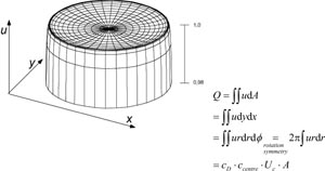
Figure 1. Basic idea of the optical-based primary flow rate standard: determination of the local velocities u in the cross section of a flow and their area integral.
Download figure:
Standard image High-resolution imageAs illustrated in figure 1, in the case of an axi-symmetric flow the area integral is then simplified to Q = 2π∫ur dr with the local velocity u as a function depending on the radius r. In a flow which is established downstream of nozzle contraction (as is the concept here, see section 2.4) we can separate the different areas along the radius of the cross section into two parts:
- The core flow which can be described as practically independent of viscous forces (potential flow, Euler flow). The mean velocity of this region can be expressed with the centre line velocity Uc and a correction factor ccentre, which is close to unity and which expresses the slight curvature of isotach lines in the core flow (see section 3). About 95% of the area in the cross section is covered by this expression.
- The boundary layer which connects the wall (adhering or no-slip condition: the velocity u[y = 0] at the wall is zero) with the core flow (u[y = δ] at the outer boundary layer limit is equal to the core flow velocity U0). The conventional concept of discharge coefficient cD is used to express the impact of the boundary layer on the total flow rate (section 4).
Finally, we obtain the working equation for the determination of the flow rate in the cross section with area Anozzle:

The main intention of this paper is to give an overview of the uncertainty budget; hence, we will give detailed explanations of the sources of uncertainty according to equation (1) and the determination of their values. This is done separately for the core flow part (ccentre and Uc; section 3) and the boundary layer (discharge coefficient cD; section 4)1.
Before this, however, we want to introduce details of the technology concept and would like to give a technical description of the facility in section 2.
2. Explanation of technology/technical description
2.1. Set-up of the installation
The optical primary standard is connected to the German gas transmission network and it uses high-pressure natural gas in a pressure range between 1.6 MPa and 5.5 MPa and flow rates up to 1600 m3 h−1. The facility entrance includes a filter to skim particles like flash rust out of the gas flow and to preserve the installations from deposits. The pressure and temperature regulation is provided by the pigsar™ system to ensure appropriate conditions for all flow rates taking gas from the upstream pipe network 'Gescher' and finally delivering into the local pipe network 'Glückauf' (figure 2). A test section with a high efficiency flow straightener can be used to prove equipment under test; length compensators (L) allow its unproblematic installation. The test section is followed by two static mixers from Sulzer, Winterthur in Switzerland [2]. Between them is a seeding device that injects small particles in the range of 1 µm used as scatterers for the optical measurement. The mixers provide a good homogeneity of the particle distribution in the flow. Behind the seeding and mixing area a Zanker-type flow conditioner diminishes the angular momentum of the flow and a diffuser enlarges the pipe diameter from DN 200 to DN 500. The connected settling pipe is a 10 m long pipe of DN 500 with the largest cross section and an inner diameter of 423 mm. The mean flow velocity in the pipe is typically 0.5 m s−1 and the turbulence intensity is expected to be as high as 30% at the first section of the pipe, but could not be measured. The pipe with a length of 24D is to reduce the pre-existing turbulence from the flow conditioner and forms a pipe flow halfway to equilibrium conditions at the entrance to the optical test section. Here, the flow exhibits the wanted rotational symmetric shape of the flow profile. At the entrance, woven wire screens mainly reduce streamwise velocity fluctuations with little effect on the change in flow direction, and reduce the turbulent boundary layer. Vortices with the size of the wires behind the screen superpose with their adjacent vortices, dissolve and homogenize the momentum. This suppresses the formation of vortices larger than the mesh size, see [3]. The boundary layer also is affected by this homogenization. The vortices from the mesh transport momentum from the core flow into the boundary layer, making it thin. A normal, new turbulent boundary layer with vortices of the order of the boundary layer thickness will form after a short settling length, see [4]. A short stilling section after the mesh allows the decaying of the small-scale turbulence of the flow that is induced by the mesh.

Figure 2. Pipework of the optical standard.
Download figure:
Standard image High-resolution imageThe LDV nozzle module with optical access to the test section and a connected nozzle bank with critical nozzles form the end of the test facility. The nozzle bank with eight nozzles sets the flow rate and serves as a transfer standard to the volumetric flow standard High-Pressure Piston Prover (HPPP, see figure 23) and also stabilizes the flow during the optical measurement.
2.2. Seeding
Optical methods for measuring the flow velocity need a sufficiently large number of particles with a known size distribution. Because of the high pressure in the pipe flow, a Laskin nozzle aerosol generator for high-pressure seeding has been developed. The use of a slit-type nozzle increases the dispersed phase production and reduces the volume of compressed air required, see [5]. The nozzle with its jet impactor plate operates below the liquid surface in the pressurized vessel. The nozzle is constructed for a pressure difference of up to 2.0 MPa between the nozzle and the seeding fluid. The vessel has two glass sight funnels to check the liquid level and to see if the system is operating properly. In order to reduce—in the small internal space of the vessel—the effect of splashing and to separate large particles, a perforated baffle was placed in front of the output [5].
For the production of particles, an overpressure of the carrier gas to spray the seeding fluid is necessary. The real gas from the facility is taken as the carrier gas. Laskin-type aerosol generators show a linear production rate with pressure while maintaining a homogeneous particle size distribution. For a slit-type nozzle with a 100 µm slit and a 1 l quantity of seeding fluid in the vessel, operation has shown that about 0.1 MPa gauge pressure is sufficient for the particle rate needed, which is equivalent to about 2 ml h−1 of fluid.
The working pressure at the facility is operated from 1.6 MPa to 5.5 MPa. To obtain a gauge pressure of 0.1 MPa for the aerosol generator, a pressure difference regulation valve was inserted in the pressure supply. In case of operation needed at very high pressures, a reciprocating gas compressor driven by the high-pressure gas supply can be switched on. The aerosol generator is designed for operating at up to 10 MPa; the vessel conforms with the European pressure equipment directive (PED) and is approved for application in real gas facilities. The nature of the seeding fluid used is di-ethyl-hexyl-sebacate (DEHS) with a density near that of water (figure 3).

Figure 3. Pressurized vessel of the aerosol generator with a slit-type nozzle.
Download figure:
Standard image High-resolution imageThe aerosol generator is supplied with a differential pressure regulator valve that maintains the set differential pressure between the inlet pressure and the outlet pressure of the aerosol generator when the working pressure of the pipe facility is changed and also functions independently of the input pressure of the high pressure supply. The additional gates in figure 4 are used for refilling the seeding fluid as well as venting (safety shut-off valve SAV) and pressurizing the generator and for safety purposes (return valve RV).
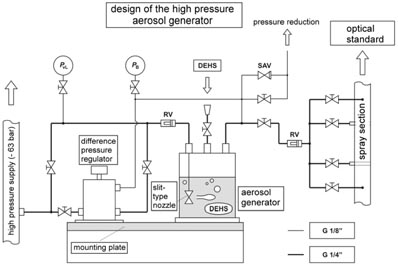
Figure 4. Configuration of the pipework of the aerosol generator.
Download figure:
Standard image High-resolution image2.3. LDV nozzle module
A nozzle contraction ratio c = 18 was designed to cover the flow rate range of all G1000 working standards used by pigsar™ (100 m3 h−1 to 1600 m3 h−1, see figure 23) in such a way that the maximum velocity at the nozzle outlet does not exceed approximately 50 m s−1 for the selected flow rates. This ensures optimal conditions for LDV signal acquisition. The nozzle was designed as a compatible insert of the LDV nozzle module. The module is fitted with two high-pressure glass windows to provide the optical access required for LDV velocity measurements at the nozzle outlet surface. The flow temperature is monitored with a PT100 inside the wall of the nozzle's throat. Additionally, the temperature balance at all points of temperature measurement upstream and downstream of the optical-based system (see figure 2) is kept within 0.2 K to ensure an uncertainty of temperature measurement below 0.1 K. The static pressure is read at the inlet of the nozzle and through four static pressure holes of 1 mm in diameter at the nozzle exit.
A diffuser is installed downstream of the nozzle (to the right in figure 5) to ensure further downstream flow stability. With optical access, it is possible not only to operate a standard LDV to measure the centre line velocity, but also to use the optical boundary layer sensor to investigate small profiles.
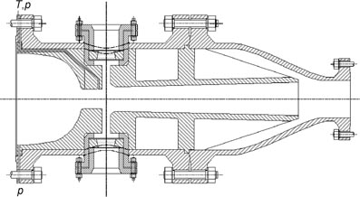
Figure 5. LDV nozzle module with the nozzle for 100 m3 h−1 to 1600 m3 h−1 (c = 18).
Download figure:
Standard image High-resolution imageA bank of eight critical nozzles was installed in the pipework covering a flow range from 25 m3 h−1 to 1600 m3 h−1. The position of the nozzles was selected so that they can be operated in series either with the piston prover, the new optical standard or the two new meter runs. AGA-8 calculation algorithms are implemented in the data acquisition system in order to calculate the critical flow factor c*, the thermodynamic property essential to critical nozzle mass flow measurements. Temperature and pressure are measured at each nozzle, and gas composition through an online process gas chromatograph. The function of the critical nozzles is manifold: firstly, they simply stabilize flow, which is important for LDV measurements. Secondly, the critical nozzles represent secondary standards of pigsar™. They make it possible to compare the two primary standards and check the reproducibility of the working and primary standards.
2.4. LDV nozzle
The measurement of flow rate in a turbulent pipe flow by integrating the flow velocity over the pipe area with the requirement of a low uncertainty is not compatible with short measuring times because of the level of turbulence. Hence a nozzle is a way of shortening measuring times. A nozzle contracts the flow by converting the pressure into kinetic energy. The right shape of its contour contributes to the same amount of pressure conversion for all streamlines and if the energy increase is homogeneous in the main flow, the velocity differences in the nozzle exit will be small. A higher contraction causes a more planar velocity profile.
The computation of a large number of nozzle shapes undertaken by Börger [4] resulted in a set of profile parameters for different Reynolds numbers and contraction ratios that have been adapted to the LDV nozzle.
For the optimization of the nozzle contour a potential flow inside the nozzle has been assumed. The calculus uses a singularity model. The walls have been replaced by vortex layers; at the inlet is a source disc and at the outlet of the nozzle is a sink disc. The wall friction was taken into account by boundary layer calculations using the method of Bradshaw et al [6]. A profile is regarded as optimized when—in the exit of the nozzle—there is a plane velocity distribution within 0.1% and when—in the boundary layers of the contour—the friction coefficients are larger than 0.002 to suppress flow separation [6].
A nozzle with a diameter of 100 mm (see table 1) has been manufactured and the nozzle exit plane roundness has been calibrated by PTB Department 5.3.
2.5. Conventional LDV
The optical flow rate measurement is traced back to a precise velocity measurement at the LDV nozzle outlet of the LDV nozzle module (figure 5). The velocity u of the gas flow is measured by a dual scatter LDV based on the differential Doppler technique and is determined by

with fD as the Doppler frequency of the measuring signal generated by the scattered light of tracer particles embedded in the flow and d as the fringe spacing in the LDV measuring volume.
The measuring volume is given by the intersection volume of two laser beams crossing each other at an angle of ε. The fringe spacing is ideally given by
For a well-aligned optical set-up and Gaussian beams crossing each other at their beam waists, the fringe spacing is constant within the measuring volume. This is not the case when thick windows for optical access have to be used. Thus, the LDV has to be calibrated including the high-pressure glass window. The calibration is done by measuring the local fringe spacing and determining its deviations over the length of the measuring volume. The deviation of the fringe spacing within the measuring volume determines the uncertainty of the LDV velocity measurement and also gives the impression of a non-existing turbulence intensity of the flow. The LDV with a wavelength of 852 nm and a power of 26 mW was used in a forward scattering mode. The focal length of 600 mm generates a fringe distance of 10.2 µm, a diameter of 163 µm and a length of 4 mm of the measurement volume (figure 7). This allows the LDV to measure in the centre of the flow as near as 7 mm from the nozzle exit plane.
The calibration method is to generate precise particle velocities and to measure the Doppler frequency in order to calculate the fringe spacing at different positions of particle transitions in the measuring volume. The most precise method is to use single particles on a rotating glass wheel with its well-known diameter. The wheel is driven at a constant rotation speed by a stepping motor to ensure a very smooth and accurate circumferential velocity. After calibration of the LDV, the LDV and its power supply are installed in a container that protects them from explosion risk in the zoned area 2. The container with the LDV inside is installed at the window of the nozzle module (figure 6) and is flushed with nitrogen before operation. The velocity signals of the LDV are sent via a 30 m long fibre optical cable to the signal acquisition system.
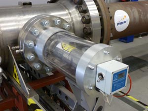
Figure 6. LDV adapted to the nozzle module.
Download figure:
Standard image High-resolution image
Figure 7. Schematic diagram of the position of the measuring volume in the centre streamline of the nozzle.
Download figure:
Standard image High-resolution imageThis LDV system has been used in backscatter mode in order to monitor the centre line velocity of the top-hat profile of the nozzle and is designed to have access to the centre of the nozzle flow only.
2.6. Boundary layer LDV
The boundary layer LDV has to measure the shape of the boundary layer at the nozzle exit. The spatial resolution of conventional laser Doppler systems is limited by the dimensions of the measurement volume. In applications with high velocity gradients such as in boundary layers, the integration of the local velocity over the extension of the measurement volume cannot be neglected. The method used locates the particle trajectory inside the measurement volume [7].
Instead of analysing the scattered light from two beams (dual backscatter mode), only the scattered light of the illuminating beam is analysed with light from a reference beam (reference beam technique). The reference beam is sent parallel and 2 mm downstream of the nozzle exit plane, whereas the illuminating beam intersects the reference beam near the wall of the nozzle exit. Inside the reference beam leaving the nozzle area, a fibre bundle is placed to receive the light of the reference beam as well as scattered light from the illuminating beam (figures 8 and 9).
Figure 8. Receiver bundle in the reference beam of the LDV. The fibre diameter is 1 mm. Each fibre here is illuminated with a different colour.
Download figure:
Standard image High-resolution image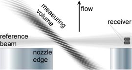
Figure 9. Schematic set-up of the boundary layer LDV.
Download figure:
Standard image High-resolution imageEach fibre of the bundle 'sees' a slightly tilted virtual fringe system and fringe distance di in the illuminating beam, and the phase differences Δφ between pairs of signals are used to calculate the position z of traversing particles in the nozzle exit plane. Three of the fibres have been utilized in order to increase the phase resolution by a factor of two and for a better signal validation and noise reduction [8].
With the distance r of the measuring volume to the receiver and the distance D between the receivers, the position z to the crossover point of the beams is

The fringe distance d'(z) of the multiple reference beam LDVs shows a small gradient that can be corrected by

Because the fringe distances di of the fibres are slightly different from each other, they have been synchronously calibrated with a calibrated standard LDV in the centre of the nozzle (figure 10).
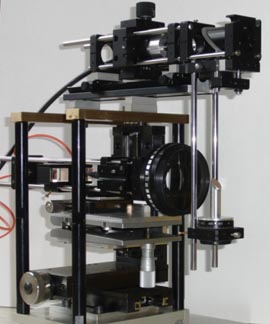
Figure 10. In the lower part of the figure is the calibrated standard LDV, in the upper part of the picture is the receiver module of the boundary layer LDV.
Download figure:
Standard image High-resolution image2.7. Calibration of the LDV
To ensure traceability to the units 'metre' and 'second' for the measurement of centre line velocity, the LDV was properly calibrated by measuring the local fringe spacing and determining its deviations inside the region of the measuring volume where the intensity of light is larger than 1/e2 of the maximum value.
The calibration method used to measure the local fringe distance is to generate precise particle velocities and to measure the Doppler frequency in order to calculate the fringe spacing at different positions of particle transitions along the measuring volume. We used single particles on a rotating glass wheel with its well-known diameter driven by a stepping motor to ensure a very constant and accurate speed. For the calibration of the LDV the high-pressure glass window, which is used at the test section, was included. The equipment and a detailed uncertainty budget for the particle velocity on the glass wheel are given in [9].
Calibration of the LDV is done according to the relevant calibration and measurement capability (CMC) of PTB (see Key Comparison Database [KCDB], 9.7.1, DE39) with an expanded uncertainty of U = 0.11% including a term of reproducibility checked by four repeated calibrations in a time scale of several weeks.
3. Core flow characteristic
The characteristic of the core flow is established by the shape and contraction ratio of the nozzle (see also section 2.5). The intention to make use of a nozzle is to obtain a velocity profile where the local velocity is nearly constant all over the core region and the local turbulence intensity is small. As one can see in figure 11 this was achieved quite well for our experimental set-up. With this behaviour it is reasonable to make use of the centre line velocity Uc for the calculation of the total flow rate QV using the relationship
 . The factor ccentre is therefore a kind of calibration factor which is determined based on the measurement by means of LDV and has in our case a value very close to unity with ccentre = 1.000 68.
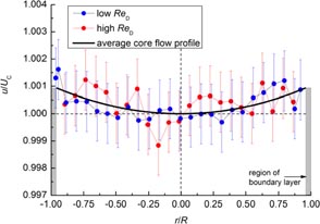
Figure 11. Core flow characteristic: each value of local velocity is the average of roughly 250 to 300 single velocity measurements with LDV. The error bars indicate the finally estimated expanded uncertainty of 0.11% for the measurement of velocities in the core flow.
Download figure:
Standard image High-resolution imageThe maximum relative difference between the centre line velocity and the outer region of the core flow is 0.1% and the overall shape is typically for the curvature of isotach lines in a flow with nozzle contraction. This part of the flow can be described by non-viscid potential flow and is practically constant in our range of Reynolds numbers. With a certain minimum set of measurements across the nozzle, the average core profile can be determined with a sufficiently small uncertainty. The description of the average core profile in figure 11 can be performed by a quadratic function2 for which the confidence interval (95% coverage) could be evaluated as 0.015%.
The core flow was measured with a conventional LDV (see section 2.6) and, for the uncertainty, we have to discuss two further points:
- the dependence of the centre line velocity on the location downstream in the flow direction in the nozzle free stream (because we did not measure exactly in the exit plane of the nozzle) and
- the optical impact of the thick glass windows on the velocity value measured with the LDV.
For the first point we proved that the centre line velocity is practically independent of the downstream location in the very first part of the near field of free stream where we applied our measurements. The results for this are shown in figure 12. The invariance could be evaluated with a 95% confidence (uncertainty) of also 0.015%, so that we get finally a level of 0.021% for the expanded uncertainty of the factor ccentre (root sum square of two independent contributions to the uncertainty).
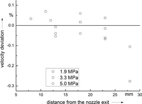
Figure 12. Variation of the centre line velocity in the free stream flow downstream of the nozzle exit.
Download figure:
Standard image High-resolution imageThe second point is more critical regarding the uncertainty. As is to be seen in figure 11, the local velocity measured by means of the LDV scatters in an interval larger than the uncertainty we figured out for the factor ccentre. The behaviour of the scatters and their distributions indicates that this is not caused by the behaviour of the flow but has its reason in the characteristic of the optical access to the flow through quite thick glass windows. There are two sources of impact on the optical behaviour of the laser beam and therefore on the uncertainty of velocity measurement in the core flow. Both are illustrated in figure 13. Figure 13 (left part) shows the polarization effects of light due to mechanical tensions in the glass; figure 13 (right part) gives an impression of the number and the size of droplets which can be found at the inner surface after several hours (here about 20 h) of operation. With this background it is easy to understand why the velocity value changes rapidly if the location of velocity measurement is changed only a little because the laser beams pass the window at different locations where the impact on the wave fronts (and therefore on the calibration value of the LDV) is significantly disturbed. From data as given in figures 11 and 12 we derived an uncertainty in the order of 0.1% (level of scatters around the average of core velocity profile). Hereby, it is necessary to ensure that the window surface is checked for its quality (sufficient short intervals of cleaning, scanning of a minimum region to ensure the use of areas with different polarization effects).
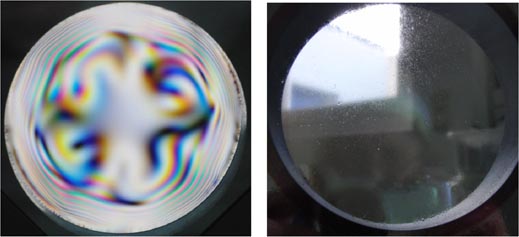
Figure 13. Optical imperfections of the glass window in the optical standard under high pressure, left: polarization effects due to tensions in the glass; right: droplets on the window surface after a longer time of operation (about 20 h).
Download figure:
Standard image High-resolution imageThe local scatter of velocity measurement in the core flow by an order of 0.1% is one of the main sources of uncertainty for the centre line velocity and therefore for the volume flow rate of the optical primary standard (see table 3 in section 5).
The core flow in figure 11 has been measured about 7 mm downstream of the nozzle to control the flatness of the profile with a conventional LDV, also the centre line velocities in figure 12. Similar measurements have been carried out at 1 mm downstream of the nozzle exit plane by moving the boundary layer sensor. In our set-up both LDVs had their measuring volume at the same place, see figure 10. The boundary layer sensor's fringe distance was calibrated with the conventional LDV at a minimum distance downstream of the nozzle where both sensors did work.
4. Determination of the boundary layer velocity profile
The determination of the boundary layer velocity profile is directly related to the determination of the discharge coefficient cD in equation (1). One of the characteristic values which describes the boundary layer is the displacement thickness δ*; see figure 14 and equation (6). With equation (7) the final relation of the boundary layer and the discharge coefficient cD is given.


A first estimation3 with cD ≈ 0.99 yields δ*/R ≈ 0.005 for the displacement thickness and we get Reynolds number
 values in the range of 1100 to 41 000 for the nozzle of the optical standard. This indicates that turbulent boundary layers can be expected for all profiles because the limits for laminar layers are exceeded by a factor of at least4 two.
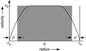
Figure 14. The displacement thickness δ* connects a real (viscid) flow profile to an ideal (non-viscid) flow profile and is related to the discharge coefficient of the nozzle flow according to equation (7).
Download figure:
Standard image High-resolution imageIf we look at one example of collected data measured by means of the boundary layer sensor in figure 15 we can find the following challenges:
- We have large sets of single data (several thousand to several tens of thousands) with large (turbulent) scatter on the length scale (sy) as well as on the velocity scale (su) which makes the handling of some operations very time consuming.
- We cannot directly measure the velocity zero (the minimum is practically about 0.1U0).
- Even had we measured the velocity zero, this would not be the condition at the wall. Although the boundary layer sensor is located as closely as possible to the nozzle edge (see figure 9) there is a gap of about 0.5 mm to 1 mm. Hence, we measure at the very beginning of the free stream and there is definitely an influence caused by the vortex outside of the nozzle. We have to determine the limit position of this influence and have to extrapolate a certain part of the profile.
- The location yw of the wall in the arbitrary coordinate system of the boundary layer sensor could not be determined and was also moving because of changes in the refractive index due to pressure and density changes. This value had to be determined from the profile data too.
To achieve a better handling of the data, we applied the first data reduction by means of averaging the single data measured with the boundary layer sensor. After this we were able to apply two different approaches for the determination of the velocity profile in the boundary layer with respect to the established theory of boundary layers.
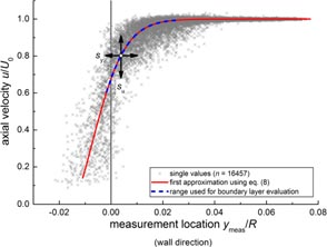
Figure 15. Example of measurement data sampled by means of the boundary layer LDV and first approximation by means of a modified hyperbolic tangent function (equation (8)) (ReD = 8.2 × 10⁶; Q = 1050 m3 h−1; p = 3.3 MPa).
Download figure:
Standard image High-resolution image4.1. First data reduction
The description of the local mean velocity in turbulent boundary layers as a function of the wall distance y is always related to logarithmic dependences (see for this especially the universal logarithmic law of the wall, e.g. [10]). The reduction of large sets of single data should therefore have a relation to logarithmic or exponential functions but should additionally have good flexibility to fit to experimental data and should have a reasonably small number of parameters. The choice in our case was a modified hyperbolic tangent function as given in

The parameters U0 (velocity at the outer edge of the boundary layer) and yw (position of the wall in the coordinate system of the optical boundary layer LDV) are general values for each velocity profile measured. The parameters k and b in equation (8) are determined by means of a non-linear least-squares fit to adapt the specific shape of the velocity profile5. Figure 15 shows one very typical example of such an approximation.
With the functional representation of the mean velocity according to equation (8) we obtained a good base for the determination of further important data as is illustrated in figure 15. The first additional data were the local fluctuations in the velocity component su (turbulent intensity in the flow direction) at a specific measurement location in the wall direction. The second were in a similar way the local fluctuations in the location ymeas for a specific level of mean velocity u/U0 in the flow profile. This second value sy does not yet have an established use in the literature. It is quite a new situation generated by the features of the boundary layer sensor and we have to emphasize that this additional information was the main basis for the successful treatment of all data.
The first important conclusion drawn from the data sy was the determination of the limit location up to where the boundary layer of the nozzle flow was influenced by the free stream vortex. As one can see in figure 17, the dependence of the local fluctuation sy shows a good self-similarity for all profiles (by means of normalization with the boundary layer thickness δ) and all profiles have a significant local minimum of sy at the same (normalized) location. We assume a no-slip condition at the wall for the nozzle flow and therefore the turbulent fluctuation has to decrease continuously to zero towards the wall. Hence, this local minimum indicates the limit position of the free stream vortex influence, which causes this deviation from the expected behaviour of nozzle flow. With this information (available separately for each profile) we were able to determine the range of the mean velocity profile, which we can use for further calculations assuming a conventional wall bounded nozzle flow (blue dotted part of the mean velocity profile in figure 15). The upper limit of the mean velocity profile usable for the subsequent calculations was set at the location of u/U0 = 0.995 because the hyperbolic tangent function does not provide a limited boundary layer u/U0 = 1 at y = δ as is necessary for our calculation approach (see the following section).
4.2. Turbulent boundary layer profiles
The turbulent boundary layers have been the subject of a very large number of experimental investigations and detailed analyses in the past which have led to well-established half-empirical models6. We will focus here only on those approaches which were finally important for our solution because it is impossible to give a comprehensive overview of everything (for this please refer to the standard literature, e.g. [10]).
For all turbulent boundary layers with no-slip condition at the wall, general behaviour of self-similarity was found if the velocity profile is normalized with the appropriate characteristic values:

where uτ is the so-called wall shear rate (or wall shear velocity), δ is the boundary layer thickness (location y = δ where u/U0 = 1) and ν is the molecular kinematic viscosity of the fluid).
Equation (9) splits the boundary layer into an inner part Gi(y+) and an outer part Go(y/δ). The inner part is described by the well-known logarithmic law of the wall and the outer part is described by the velocity defect law. The logarithmic law of the wall has a universal character for turbulent shear layers with no-slip condition but the velocity defect law is specific for a certain type of flow configuration. Nevertheless, for a given flow configuration also the outer part follows the rules of self-similarity.
The most common starting point for the description of mean velocity in the boundary layer is the basic relationship between the total shear stress τtotal, the mean velocity gradient and the turbulent shear stress 〈u'v'〉:

The turbulent shear stress 〈u'v'〉 (correlation between fluctuation of velocity in the main flow direction and direction normal to the wall) is, in most cases, not measured and not known; therefore, we have here the key point for the different approaches to describe the boundary layer by modelling. The oldest and most simple (algebraic) models7 are the concepts of eddy viscosity νturb introduced by Boussinesq [11] and the mixing length lm by Prandtl [12] with which equation (10) is reformulated as
A normalization using the molecular kinematic viscosity ν, the shear stress rate uτ and the wall shear stress
 yields

The concept of mixing length introduced by Prandtl [12] is perhaps the best known because, with the simple modelling of the mixing length using the wall distance and the empirical constant κ (introduced by Karman [13])

there is a short and direct way to the basic formulation of the logarithmic law of the wall:

As mentioned above, the logarithmic law of the wall is valid in the inner part of the boundary layer but not in the outer part. Consequently, for the complete boundary layer a model approach for either the eddy viscosity νturb or the mixing length lm as a function of the overall location of the layer is necessary. Established models for this are given by Cebeti and Smith [14] and by Baldwin and Lomax [15] for the eddy viscosity as well as by Michel [16], Escudier [17] and Szablewski [18] for the mixing length. All of them have in common that in the inner part (small values of wall distance y, smaller than a certain distance yi/o), equations (13) and (14) are valid. The modelling of the eddy viscosity by [14] as well as [15] in the outer part of the layer is characterized by a significant decrease in the viscosity for larger distances to the wall. The models for the mixing length operate with a constant mixing length lm,o in the outer part which is in the order 0.04δ to 0.09δ.
As mentioned above, the self-similar outer part of the boundary layer is specific for a certain type of flow configuration. Therefore, these established model approaches to cover the inner as well as the outer part do not give necessarily reliable solutions for all cases. And in fact, the trial to fit our boundary layer profiles with the models using a constant mixing length for the outer part did not lead to a sufficient solution.
It is, nevertheless, necessary to make the choice of an algebraic model and to determine the triple value [uτ, δ, yw]8 for each of the profiles being measured so that the experimental data of mean velocity are well represented by the model function for local velocity u versus wall distance y.
Any approach which we can choose here will make use, more or less, of some information based on the established half-empirical solutions out of the literature. This generates an additional challenge to our central aim of realizing a real independent optical primary flow rate standard. All information which we introduce or which we make use of has to be evaluated finally with its uncertainty and its impact on the uncertainty of our final measurand. This is not possible for most of the information from the literature. For example, one can look at the van Driest constant A+ and the Karman constant κ (see equations (15) and (16)). These constants are determined to fit the related models to experimental data. Although it seems that these constants have a universal character, there is an impressive discussion about their values which can vary more or less in the publications depending on the specific conditions of the experiment or the measurement. To get an impression one can refer to [19] (κ and A+) as well as [20] (κ)9.
To overcome the latter problem, two approaches will be applied and will be fitted to our experimental data; both approaches will use different sources of information from our experimental data as well as out of the established descriptions of boundary layers. The final evaluation of uncertainty for the discharge coefficient cD then involves the differences resulting from the two approaches.
4.2.1. Approach 1: self-similarity in the region of defect law.
The first approach sets the self-similarity of the velocity profiles in the defect law region into the focus. We determined the related triples [uτ, δ, yw]i for all individual profiles10 so that they collapsed early into one normalized profile from a certain common location y ⩾ yi/o. This is shown as a blue curve in the defect law model in figure 16, the normalized self-similar velocity profile needed to be adapted to the wall (y = 0) and to the core flow.

Figure 16. Presentation of 21 self-similar boundary layer profiles in the velocity defect law model using optimal values for shear stress velocity uτ, boundary layer thickness δ and position yw of the wall in the coordinate system of the boundary layer sensor.
Download figure:
Standard image High-resolution imageThe adaption to the wall has been based on the basic concept of the mixing length in the region of the logarithmic law of the wall with a transition to the region of the defect law. We give here the formulation of Szablewski [18] for the mixing length (equations (15) and (16))11,12:


According to equation (12) there is also the need to define the total shear stress τtotal as a function of wall distance in the region where we want to apply the mixing length model. It can be assumed that near the wall the total shear stress is a linear function with a gradient slightly below zero13, see also figure 20.
All together we obtained 65 parameters which had to be optimized by means of least-squares principles to fit our experimental profile data: 21 triples [uτ, δ, yw]i, the common transition point yi/o/δ between the inner and outer parts of the boundary layer and the gradient of the total shear stress near the wall. The boundary conditions for the optimization are, besides the best collapsing of experimental data to an average profile, the smooth connection of the near wall function (equations (15) and (16)) to the outer part at yi/o/δ in the local velocity as well as the first derivative of velocity.
As mentioned in section 4.1, the representations of experimental data by the hyperbolic tangent function (equation (8)) were used up to velocities u ⩽ 0.995U0. To close the last gap to the core flow we applied a simple third-order polynomial as given in equation (17):

with values of a0 to a3 so that the adaption is smooth up to the first derivative at y/δ = 0.75 and at y = δ (with additional condition U0 = u at y = δ).
The result of the whole process is shown in figure 16 using the velocity defect model. It documents the very good agreement of the experimental velocity data with the rules of self-similarity. The near wall region (which is not supported by measured data and which we modelled using the mixing length model) covers about 10% of the boundary layer. Due to the velocity gradient in this part, this implies that about 35% to 38% of the discharge coefficient is directly dependent on the quality of the near wall model. This illustrates the necessity to verify these results by another approach which is explained in the following section.
4.2.2. Approach 2: modelling of the kinematic eddy viscosity.
The second approach is based on modelling the eddy viscosity νturb in the boundary layer. The concept of eddy viscosity was introduced by Boussinesq [11] and derives from a similarity consideration of viscosity in kinetic gas theory where the molecular kinematic viscosity is derived from the relation of viscosity ν with the average molecule velocity
and the average free path length λ yielding
 . Boussinesq set the turbulence intensity equivalent to the molecule velocity and the free path length to a certain length scale lMFW which is a characterizing parameter of the turbulent flow:
 ; λ ⇒ lMFW. The length scale lMFW is in close relationship with the mixing length which was introduced later by Prandtl [12].
It is a new and unique situation that the application of the boundary layer sensor (section 2.6) allows us to derive two additional values out of the velocities usable to establish a quite similar approach: the standard deviation of velocity fluctuation su (which is identical to conventional turbulence
 and the standard deviation of location sy (which has a similar meaning to su but for the length), see for this also figure 15. We will now define the turbulent kinematic (eddy) viscosity νturb proportional to the product of sy and su for reasons of consistency of physical units:

The task is to determine for all profiles the related values of sy and su as well as the proportionality factor α14. We were starting with the assumptions that sy and su follow the basic rules of self-similarity as well as that the proportionality factor α is a characteristic constant valid in the whole range of boundary layers and for all profiles out of the same flow configuration.
The self-similarity of the normalized values of sy and su is demonstrated in figures 17 and 18. It allows the representation of sy as well as su by two general average functions versus the wall distance valid for all profiles independent of the Reynolds number. This self-similarity was consequently introduced as an additional condition for the least-squares approximation to define the best fitting parameter triples [uτ, δ, yw]i.

Figure 17. Dependence of the fluctuation in location sy of 21 boundary layer profiles normalized with the boundary layer thickness δ versus the wall distance y/δ. See also figure 15 for explanation of sy.
Download figure:
Standard image High-resolution image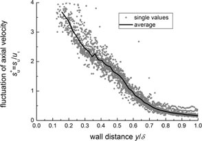
Figure 18. Dependence of the fluctuation in velocity su of 21 boundary layer profiles normalized with the shear stress velocity uτ versus the wall distance y/δ. See also figure 15 for explanation of su.
Download figure:
Standard image High-resolution imageThe general average functions for sy and su in figures 17 and 18 consequently establish the turbulent kinematic (eddy) viscosity νturb (figure 19) according to equation (18). The parameter α has to be determined so that the turbulent shear stress calculated using equation (12) fits the experimental velocity data in an optimal way. As one can see in figure 20, the total shear stress also follows the principles of self-similarity and can be represented by a general function for all profiles.
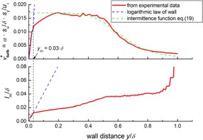
Figure 19. The turbulent kinematic viscosity and the mixing length lm determined according to equation (18) from data of turbulent fluctuation (see figures 17 and 18), normalized with boundary layer thickness δ and shear stress velocity uτ. The value for α is 0.07.
Download figure:
Standard image High-resolution image
Figure 20. Dependence of the total shear stress of 21 boundary layer profiles on the wall distance y/δ.
Download figure:
Standard image High-resolution imageThe finally determined turbulent kinematic viscosity from the experimental data in figure 19 can be compared with the values which are given by the model approach of Cebeti and Smith [14] and Cebeti and Bradshaw [21]. This approach is characterized by a viscosity νturb,∞ in the outer part (y > yi/o) which is damped towards the core flow by a so-called intermittency function:
y19 is the location where (U0 − u)/uτ = 0.19 applies according to Gersten [22].
The transition to the inner part of the boundary layer at the transition point yi/o is given where the viscosity according to equation (19) is larger than the turbulent viscosity derived from the universal logarithmic law of the wall.
We get νturb,∞ = 0.017 and yi/o = 0.03δ for our measurements which are in good agreement with the literature values νturb,∞ = 0.014 to 0.016 and yi/o = 0.032δ to 0.034δ [22] and which therefore confirm the reliability of our approach.
In figure 21 the 21 velocity profiles are shown which were calculated using the general (average) functions for turbulent kinematic (eddy) viscosity (figure 19) and the total shear stress (figure 20) according to equation (12) together with the related values for the triples [uτ, δ, yw]i and the parameter α = 0.07 (see equation (18)). The general behaviour and level of results are very close to the results obtained with approach 1 in section 4.2.1 (figure 16).
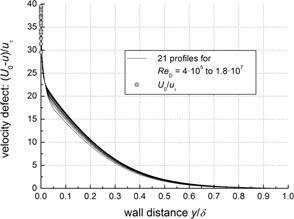
Figure 21. Presentation of 21 boundary layer profiles in the velocity defect law model calculated by means of the kinematic eddy viscosity according to equation (18), figure 19 and total shear stress according to figure 20.
Download figure:
Standard image High-resolution image4.3. Discharge coefficient and its dependence on the Reynolds number
After the introduction of the calculation of the mean velocity profiles out of the single velocity data measured by means of the LDV-based boundary layer sensor, we could get the discharge coefficient of the nozzle flow as a function of the Reynolds number directly by integrating the profiles given in the velocity defect law model (see figures 16 and 21). The results of this integration are given for all 21 profiles in figure 22 for both the first and second approaches of boundary layer calculation.
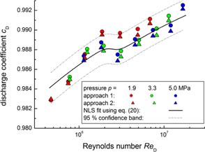
Figure 22. Discharge coefficient cD of the LDV nozzle versus the Reynolds number ReD. For the two different approaches 1 and 2, see sections 4.2.1 and 4.2.2.
Download figure:
Standard image High-resolution imageThe single results for the discharge coefficient can be summarized as a function depending on the Reynolds number because of the relation to the displacement thickness δ* (equation (7)) for turbulent boundary layers which generally follows the functionality δ* ∼ Re−n with values of n in the range between 0.132 and 0.25. We have in our case a turbulent boundary layer which is close to the situation of a layer at a flat plate15. Therefore, we adopt the value of n = 0.2 which is commonly found in the literature. The complete function describing the discharge coefficient in figure 22 is given as a set in equations (20) to (22) with related parameters (determined by non-linear least-squares fit) given in table 2.


with s1 + s2 = 1 for all Reynolds numbers ReD.
Table 2. Parameters of the function describing the discharge coefficient cD according to equations (20) to (5).
| Parameter | b1 | b2 | kTr | ReD,Tr |
|---|---|---|---|---|
| Value | 0.2146 | 0.2402 | 10 | 2.5 × 10⁶ |
It is necessary to explain why we have two different sections of cD dependence according to equation (21), which are connected by a transition function (equation (22)). As mentioned above at the beginning of section 4, the Reynolds number
—with respect to the displacement thickness—clearly indicates a fully turbulent flow regime in the boundary layer. Therefore, this cannot be the laminar–turbulent transition (this would not be compatible also because of n = 0.5 for laminar flow). The key point for the explanation is the relation to roughness. We have measured the roughness by means of a stylus instrument in some parts of the inner nozzle surface and got an average peak-to-valley height of Rz ≈ 9 µm which is in good agreement with the specification given for the manufacturing of the nozzle16. With the wall shear rate uτ and the molecular kinematic viscosity ν we obtain the normalized roughness height
 . In figure 22 it is to be seen that the transition from the first to the second part of the cD function starts at about ReD = 1.9×10⁶ (value for s1 = 0.05 and s2 = 0.95 respectively). With the related values for the wall shear rate of uτ/U0 = 0.0295 (which we got from the boundary layer calculation for the profiles at this Reynolds number) and the nozzle radius of R = 50 mm, a final value of
 results. It is a general statement in fluid dynamics (see, e.g., [10]) that a surface can be assumed to be hydraulically smooth as long as the value of
 is ⩽5. This is equivalent to the thickness of the so-called laminar (viscous) sub-layer of a turbulent shear layer at the wall. If the roughness is larger than this, then the viscous sub-layer vanishes and the wall starts to display the characteristic of a rough surface for the flow. With this we have a reliable explanation of our cD behaviour versus the Reynolds number, which reflects the transition from a smooth to a rough surface at a high level of consistency with the literature values.
The definition of the generalized cD function allows us to discuss the uncertainty of the cD calculation out of our determination of boundary layer profiles according to sections 4.2.1 and 4.2.2. Here we have to consider two parts: firstly, the differences coming out of the two different approaches for boundary layer calculation, and secondly, the deviations of the cD values for the single profiles from the generalized cD function.
The differences in the results between the two approaches for one profile do not exceed 0.05%. Hereby, the first approach made use of the mean velocity information and a simple mixing length model for the wall region only. The second approach additionally includes information about the turbulence structure based on the measurements. The results for the turbulence structure (eddy viscosity νturb) had been found very close to well-established concepts in the literature and we therefore have a high level of confidence in our results. Hence, the difference which is present in the two approaches can be used here as a measure for the uncertainty caused by the model structure for the algebraic solution of the boundary layer calculation, which is consequently conservatively estimated as 0.05% of the cD value17.
Additionally to the differences in the calculation approaches, we can derive from figure 22 that the quality of the profile measurement is different for the single profiles and generates a higher uncertainty in the order of 0.15%. This is visible in figure 22 considering the fact that the discharge coefficient should theoretically follow the straight function versus the Reynolds number as given in equations (20) to (22). For example, the cD values for Reynolds numbers between ReD = 1.9 × 10⁶ and ReD = 8 × 10⁶ for profiles measured at pressures of p = 3.3 MPa and 5.0 MPa are very close together while the values for p = 1.9 MPa differ here. The main reasons are found in the quality of optical access, which changes with operation time as was deduced in section 3 for the determination of the centre line velocity.
In total, we have to consider an expanded uncertainty of 0.154% for the cD value calculated with equations (20) to (22) to cover 95% of our experimental result. This is the largest contribution to the uncertainty budget as listed in table 3.
Table 3. Overview of the uncertainty budget.
| Component | Symbol | Estimate of expanded uncertainty U (95% coverage) | Degree of freedom | Remarks |
|---|---|---|---|---|
| Cross section of LDV nozzle exit | Anozzle | 0.021% | ∞ | Calibration certificate with CMC reference |
| Centre line velocity | Uc | Basic calibration of LDV including LDV reproducibility: 0.11% | ∞ | According to CMC of PTB including for LDV calibration |
| Optical imperfections: 0.11% | 52 | (see section 3) | ||
| Correction factor for the centre line velocity | ccentre | 0.021% | 52 | (see section 3) |
| Discharge coefficient | cD | 0.154% | 20 | (see section 4.3) |
| Total | 0.219% | 74 |
5. Overview of the uncertainty budget
From the working equation (equation (1)) for the determination of the volume flow rate at the nozzle exit we get for the propagation of uncertainty:

The sources of the uncertainty components for the discharge coefficient cD, the centre line velocity Uc and the correction factor ccentre of the centre line velocity have been discussed above in detail as far as they were derived from measurement results by means of the optical sensors and from the related data processing. They are summarized in table 3 together with those components that are directly given by other sources (calibration result based on established CMC entries).
In the ranking of the impact, the uncertainty of the discharge coefficient is the largest part followed by the centre line velocity as well as the basic calibration of the LDV. As mentioned in the related sections (sections 3 and 4.3), a key point for the uncertainty of the values is the quality of optical access. Situations as shown in figure 13 (right part) should be avoided by means of quality measures, i.e. sufficient intervals of cleaning and/or further reduction of seeding material used for the measurements. With this precondition the uncertainty can be kept within the claimed uncertainty budget of a total expanded uncertainty of 0.22% for the volume flow rate under working conditions in the optical-based primary flow rate standard.
6. Comparison with values traceable to the HPPP
After the determination of the uncertainty budget it is necessary to verify this claim by means of an intercomparison. It is a convenient situation for PTB at the high-pressure test facility pigsar™ that the new optical primary standard is incorporated into a facility with a well-established and approved system using a conventional HPPP. Figure 23 gives the flow chart of the traceability chain of pigsar™ in which we are able to compare the conventional traceability directly with the new optical standard via the pivot point of the secondary standard (critical nozzles) [33–35].
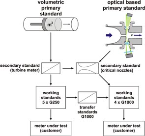
Figure 23. Traceability model of the high-pressure calibration rig pigsar™ including the optical-based primary standard [33–36].
Download figure:
Standard image High-resolution imageThe uncertainty of the conventional traceability of pigsar™ is documented in the related CMC entry of PTB for high-pressure natural gas in the KCDB of the Bureau International des Poids et Mesures (BIPM) [36]. The level ranges from 0.13% to 0.16% depending on the flow rate and includes all contributions of stability of secondary or working standards as well as the contributions of pressure and temperature measurement that are necessary to convert the volume of gas from the location of the reference standard to the location of the device under test. For our comparison we made use of the optical standard in the sense of a device under test. The indicated volume flow rate of the optical standard was therefore compared with the volume flow rate determined with the pigsar™ system (using the critical nozzles) including pressure and temperature conversion. Hence, we finally checked the relative differences Δ = ((QV,opt.Stand − QV,HPPP)/QV,HPPP) · 100% with the uncertainty UΔ given by
 where UV,HPPP is the CMC-based uncertainty of the pigsar™ facility as mentioned above and UV,opt.Stand is the uncertainty of the optical primary standard as given in table 3.
Figure 24 summarizes the results of this comparison, showing the differences Δ together with the related expanded uncertainties UΔ (error bars). The values are given again versus the Reynolds number (to keep the relation to the other graphs, especially in section 4) and cover flow rates between 100 m3 h−1 and 1500 m3 h−1 for each of the pressures. For all flow rates and pressures, the value of Δ indicates an equivalence of both values traceable to the two different primary standards (UΔ always larger than the absolute value of Δ). All considerations presented in this paper are confirmed by this result.
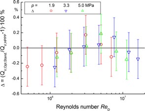
Figure 24. Differences and related (expanded) uncertainties between volume flow rates determined with the optical primary standard (opt. stand.) and based on the conventional volumetric primary standard (HPPP).
Download figure:
Standard image High-resolution image7. Summary and outlook
We have demonstrated, with a detailed explanation of the technology, the basic measurement principles and the measurement results that the new optical primary standard for the volume flow rate of natural gas under high pressures has been brought successfully into operation. For the evaluation of the uncertainty of the new system all necessary details were presented and the total expanded uncertainty of U = 0.22% for the volume flow rate under working conditions in the primary standard has been confirmed by a comparison with the established conventional traceability of PTB for high-pressure natural gas.
The level of uncertainty seems at first view not yet competitive with the established conventional technologies of primary standards for gas. We have to consider, however, that the new technology presented has a specific advantage in applications for large flow rates. The actual realization at PTB is designed to cover our need to calibrate working standards up to a flow rate of 1600 m3 h−1. But there is no reason why the same design could not be applied in a double-sized pipe system which implies operability up to 6500 m3 h−1.
The approach to apply a nozzle flow with a high contraction ratio was found helpful because it led to clearly distinguished parts of the flow which could be handled separately, the core flow and the boundary layer. The determination of the boundary layer and its characteristic parameter of the discharge coefficient is a kind of facility parameter and is mainly time invariant (as long as the nozzle and flow conditions are not changed). Therefore, once determined, it can be used during further applications of the system as a time-constant factor. The same is valid for the correction factor ccentre, which brings the centre line velocity Uc in correct relation to the flow rate. Only the centre line velocity Uc has to be measured for each application of the new system as a primary reference. The time scale of the reliable determination of Uc by conventional LDV is in the order of 1 s to 3 s and not fixed to any time interval. It is, therefore, also easily possible to apply the system as a flow rate reference in flow processes with a certain flow rate range.
We devoted a large part of the paper to the explanation of the determination of the boundary layer velocity profiles and the related discharge coefficients of the nozzle flow. In this part we addressed the most critical issues regarding the uncertainty. The discharge coefficient contributes, with 0.154%, the biggest impact to the total uncertainty; therefore, the reliability of the boundary layer determination is a key point for the uncertainty budget. We were able to show the confirmation here by the demonstration that our characterization of boundary layer is in close agreement with established theoretical-based approaches and that the results differ only in a reasonably small span depending on which information of the local velocity measurement has been involved.
If we look at potential for improvement then we have to notice two main points here: the quality of the optical access and the question of whether the measurements should be made at the transition point of a nozzle flow to a free stream. With the 'quality of optical access' we especially mean that the vortices of the separated flow in the measuring chamber lead to impurities at the glass window due to particles of seeding. A different construction may help to prolong the intervals between cleaning and/or to make the cleaning mechanically easier. The second question is related to this because it would be a significant improvement if the optical access could be designed in such a way that we would be able to measure the boundary layer in a closed conduit also under high-pressure conditions. This would provide a better definition of the wall conditions for all the processes of boundary layer determination and would therefore lead to a significant decrease of uncertainty in this area.
Footnotes
- 1
The uncertainty of the cross section area Anozzle is given by the calibration certificate (CMC supported) for the measurement of the nozzle dimensions.
- 2
- 3
We could get such an estimation if we calibrated the nozzle of the optical standard similarly to a differential pressure device using the mass flow determined by the established conventional traceability of the test facility pigsar™ (see figure 23).
- 4
- 5
The function according to equation (8) is flexible enough to represent mean velocity profiles having discharge coefficients in a wide range but the same order which we have to expect here and to ensure a realistic profile shape of boundary layers ranging from laminar to fully turbulent boundary layers. The shape behaviour was checked by means of the shape factor H12, which is the relation between the displacement thickness δ* and the momentum thickness θ of the boundary layer.
- 6
'Half-empirical' means that the models for the boundary layer flows are based on certain structures which are established using relationships of the physics and some basic assumptions (theoretical basis) and which contain parameters which have to be adopted to make the models fit experimental data (empirical basis).
- 7
We consider here algebraic models only because for other types of models such as the two-equation models (k–ε or k–ω) as well as Reynolds stress models we do not have enough information about our flow.
- 8
As already mentioned above, it was not possible to determine the exact position of the wall yw in the arbitrary coordinate system of the boundary layer sensor in an independent way. The most likely approach for such determination would be the measurement at both sides of the free stream by traversing the boundary layer sensor with the well-known diameter of the nozzle exit. But this was not successful because the boundary layer sensor was usable with sufficient performance only at the side closer to the laser source for the same reasons as we pointed out in section 3 for the uncertainty of core velocity measurement. Therefore, it was necessary to reveal the value yw also from the approximation process.
- 9
For our purposes, we applied the most conventional values κ = 0.41 and A+ = 26.
- 10
We made use of the representation of profile data by means of the modified hyperbolic tangent function after the first data reduction (see section 4.1).
- 11
- 12
The complete formulation of Szablewski [18] gives a constant value for the mixing length in the region of the defect law which is lm,Swabl/δ = κ · yi/o/e · δ for y > yi/o but we did not make use of it because the fitting with our experimental data was not sufficient. Equation (16) additionally involves a term which was introduced first by van Driest [23] to adapt the turbulent shear layer smoothly to the laminar (viscous) sub-layer.
- 13
Zero would be realized in a flow without a pressure gradient. In fully developed channel flows the gradient is equal to −1.
- 14
A first estimation of the level of the factor α can be derived from the basic relationship of the shear stress
 . Measurement results published by [27–31] gave estimations of α between 0.1 and 0.2. The best approximation of our experimental data by optimal values for the triples of [yw, uτ, δ]i led here to a value of α = 0.07, which is at an acceptable level of agreement compared with the first estimation based on the other experiments.
 - 15
The large ratio of surface curvature (pipe radius) R to the displacement thickness δ* in connection with the high Reynolds number ensures that the curvature is insignificant for the development of the boundary layer. Furthermore, the flow at the nozzle exit is not accelerated significantly. As a comparison to this one can refer to the discussion on high accelerated flows in nozzles as given in [32].
- 16
The nozzle was drilled with a specification of the arithmetical mean deviation of Ra = 1.6 µm. For drilled surfaces one has to expect a factor of about 6 between the values of Ra and Rz.
- 17
It has to be noted that we, of course, also obtained uncertainty statements for the cD values based on our least-squares approximation of all the parameters involved in the boundary layer calculation but the resulting uncertainty is in the order of 0.3% due to the large number of parameters, i.e. the triples [uτ, δ, yw], the common transition point yi/o/δ and the gradient of the total shear stress (in approach 1) or the factor α (in approach 2).