
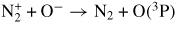
Abstract
The production process of OH radicals in an atmospheric-pressure streamer discharge is studied. A streamer discharge model is developed to analyse the characteristics of a pulsed positive streamer discharge in point-to-plane electrodes filled with humid air at atmospheric pressure. The results indicate that the behaviour of OH radicals in and after the discharge pulse is characterized by three reaction processes: 'OH-production', 'OH-cycle' and 'OH-recombination'. The first process of OH-production includes dissociation reactions of H2O with O(1D) and N2
 , which are the main production processes of OH in the discharge. Immediately after the OH-production process, the OH radicals are destroyed by a reaction with O(3P) to form O2 and H. Then the subsequent reactions produce OH again through the reaction of H + HO2, which is the OH-cycle process. Finally, the OH radicals are consumed by the OH-recombination process.
Export citation and abstract BibTeX RIS
1. Introduction
Non-thermal plasmas generated in air at atmospheric pressure have attracted considerable interest because of their non-thermal property and high reactivity [1]. A streamer discharge (e.g. a corona discharge and a dielectric barrier discharge) is one such non-thermal plasma. In a streamer discharge, chemically active species such as O, N and OH are produced, which play important roles in many applications such as the decomposition of gaseous pollutants [2], water treatment [3], ozone production [4, 5], plasma-assisted ignition [6], surface treatment [7, 8] and medical applications [9]. However, the understanding of radical production in a streamer discharge is still poor. The above applications need to be optimized in a highly scientific way to both improve the energy efficiency and confirm their safety. The authors previously clarified the production mechanism of O and N radicals in a streamer discharge in dry air by comparison between experimental and simulated results [10]. For the increased practical use of atmospheric-pressure plasmas, a discharge model under humid-air conditions needs to be developed.
The OH radical has been considered one of the important reactants in the removal of gaseous pollutants since OH has a higher oxidation potential than other oxidative species such as O, HO2, H2O2 and O3. For example, Lowke and Morrow [11] theoretically showed that OH plays a major role in removing SO2 in a pulsed corona discharge. Magne et al [12] reported that the OH radical reacts with more volatile organic compounds (VOCs) than the O radical at ambient temperatures. However, the behaviour of the OH radical is not yet well understood because of its complex reaction processes [13]. For example, in many previous studies, OH has been considered to be mainly produced by the following reactions [2, 11]:


Figure 1 shows the reaction rates of (1), (2) and the production of O(1D). These rates are calculated from the Boltzmann equation with the set of cross sections for humid-air conditions. The reaction rate of O(1D) production, and as a result the reaction rate of (3), is much faster than those of (1) and (2). Therefore, as figure 1 indicates, OH radicals are mainly produced by (3). However, this conclusion cannot explain our previous experimental results, which show that almost the same amount of OH is produced in humid-air and humid-nitrogen discharges [14]. The following reaction has been suggested as a major production channel of OH radicals in humid nitrogen [15, 16]:

The production rate of
 by electron impact is also shown in figure 1. It is over an order of magnitude slower than the production rate of O(1D) and four orders of magnitude slower than that of (3) [16]. Therefore, (4) cannot be substituted for (3) as a major OH-production reaction channel in humid nitrogen.

Figure 1. Dependence of reaction rates (kδ) with mean electron energy under humid-air (H2O = 2.0%) conditions where k is the reaction rate constant by electron impact and δ is the fraction of nitrogen, oxygen or water in the mixture.
Download figure:
Standard image High-resolution imageThe discharge propagation kinetics in humid air is also complicated. Even a small amount of humidity in air strongly affects the electron transport coefficients, such as drift velocity and mean electron energy, because H2O molecules have a large cross section at low energies (<1 eV) owing to their high dipole moment [17]. In addition, the humidity accelerates vibrational relaxation rates and therefore increases the gas temperature after the discharge [18, 19]. Moreover, some discharge products derived from H2O such as H, HO2 and H2O2 are also reactive and have been reported to have important roles in the discharge kinetics [12, 15]. However, these effects have not been sufficiently confirmed.
In this paper, the streamer discharge kinetics in H2O/O2/N2 is analysed using our previously developed two-dimensional streamer discharge model. In particular, the behaviour of OH radicals is discussed by comparison between experimental and simulated data. Then, the mechanism of OH radical production is discussed.
2. Kinetic model
2.1. Discharge model
The simulations are performed in a 13 mm-gap point-to-plane electrode configuration according to our experimental setup. Streamer dynamics are described by the following system of equations:


where ns, vs(E/N), Ss(E/N), μs(E/N) and Ds(E/N) are the charged particle density, charged particle velocity, particle chemical source term, mobility and diffusion coefficient, respectively. The subscript 's' denotes electrons (e) or positive (p) or negative (n) ions. E is the electric field, ε0 is the permittivity of free space, and e is the absolute value of the electronic charge. The transport and source parameters involving electrons (such as ve, De, and the reaction coefficients in Ss) are calculated using Bolsig+ software [20] with previously published e-V cross sections [21]. A detailed description of the chemical reaction model is given in the following section. In (7) and (8), all ion mobilities are assumed to be 2.2 × 10⁻⁴ m2 V−1 s−1 [22]. This assumption is a rough estimation because ion mobilities are a function of reduced electric field E/N. However, since it is commonly accepted that the ion mobilities are significantly slower than the electron mobility due to a much larger mass, the ions hardly move (remain relatively static) within several nanoseconds. A similar value of ion mobility is used by Morrow and Lowke [23]. Ion diffusion is neglected for the same reason. Photoionization is taken into account through the three-exponential Helmholtz models [24, 25]. Equations (5) and (9) are solved using a general personal computer in an attempt to reduce the computational cost. Some numerical techniques such as the method of solving (5) and (9) are given in our previous paper [10].
Figure 2(a) shows the configuration of the electrodes and the computation domain. To simulate the development of a discharge, we chose a cylindrical domain of 18 mm height and 8 mm radius. The total number of grid points is Nz × Nr = 1792 × 256 with spatial steps from δz = 1 µm (near the point anode and plane cathode) to 10 µm (at the interelectrode gap) [26] in the z-direction and from δr = 2.5 to 200 µm in the r-direction. The spatial resolution is derived from Eichwald et al [27]. The point electrode has the form of a hyperboloid of revolution with a radius of 40 µm, corresponding to that used in our experiment. At the conducting anode, the positive ion fluxes are fixed to zero, while the negative ion and electron fluxes are estimated using the Neumann boundary condition [27]. At the conducting cathode, the Neumann boundary condition is applied to all positively and negatively charged fluxes [27]. All radial derivatives of the densities are set to zero at the open boundaries [28]. Figure 2(b) shows the waveform of the applied pulsed voltage and figure 2(c) shows an enlarged view of figure 2(b) and the discharge current calculated by an extension of Morrow and Sato's formula [29]. In this simulation, the actual pulsed voltage, which is measured from our experiments, is applied to the conduction anode tip. The discharge voltage V, which is set to 24 kV in figure 2(b), is defined by the peak voltage of the pulse. The rate of voltage increase is about 0.52 kV ns−1.
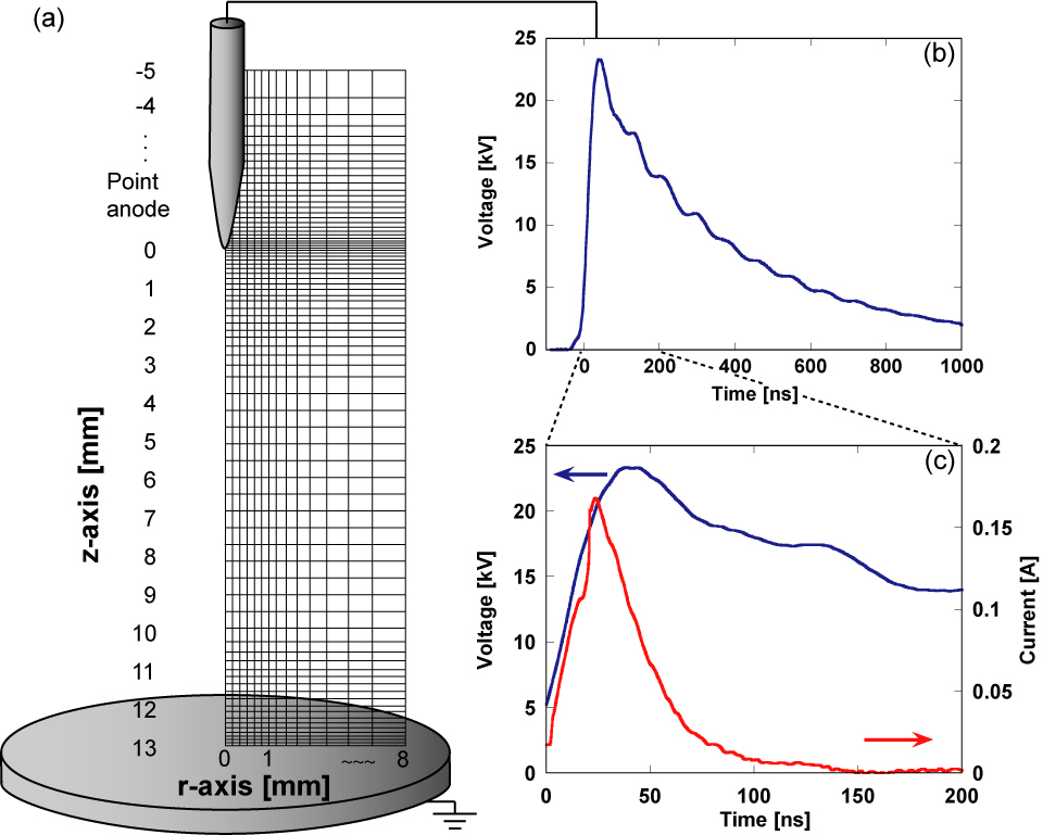
Figure 2. (a) Schematic view of the calculation domain and mesh, (b) waveform of the applied pulsed voltage and (c) enlarged view of the applied voltage and calculated discharge current. The applied voltage is 24 kV.
Download figure:
Standard image High-resolution imageIn our simulation, the neutral particles are assumed to be static. Much work remains to be done on the questions of gas heating and the decrease in gas density, which affect the electron distribution function through the variation of reduced electric field, E/N, and the Arrhenius constant through the gas temperature [30]. Actually, it has been suggested that the decrease in density due to gas heating is responsible for the formation of sparks, initiated by a discharge [31]. However, Popov [32] estimated that the gas heating is equal to 22–26 K at 3 µs under the same conditions as this paper, and the main heating occurred after the discharge (time t > 200 ns). Therefore, it is estimated that the gas heating does not affect the electron distribution function through E/N variations in the single discharge. At t > 3 µs, the V–T relaxation through H2O molecules [18] can cause gas heating, which may affect Arrhenius constants through the gas temperature. Therefore, we compare the simulated data with the experimental data up to a time 3 µs after the discharge, which is considered to correspond to the pre-diffusion phase of neutral species in the discharge of a single-pulse streamer [33, 34].
2.2. Chemical reaction model
We used a reduced reaction model including electron impact reactions (excitation, ionization, dissociation, recombination, attachment and detachment), ion recombination and the reactions of neutrals as shown in tables 1–3. For N2 and O2 molecules, the excited species correspond to effective states clustered around actual molecular levels as described in table 4, in accordance with the method proposed by Fresnet et al [35]. The rate constants of the electron impact reactions are calculated by an analysis of the Boltzmann equation. The effects of superelastic collisions induced by highly vibrationally excited molecules on the electron energy distributions (EEDF) are not considered in this simulation because the densities of vibrationally excited molecules are relatively small and have little effect in a single atmospheric-pressure pulse discharge [10, 36]. However, superelastic collisions are expected to have an effect under low-pressure discharge or repetitive discharge conditions [37, 38]. In the charged-particle kinetics, three positive ions:
 ,
,
 and H2O+, four negative ions:
 , O−, OH− and H−, and electrons are considered. Complex ions such as
 ,
,
 and
N2, and the charge transfer reactions are not considered in this simulation. Reaction kinetics and rate coefficients of complex ions have been studied in many papers [39–42]. However, the effects of complex ions on radical production have only been investigated in simulated cases [43], and corroboration must be made through actual experiments. Even without such complex ions, the development of primary and secondary streamers was well reproduced in our reduced model, whose validity was confirmed by comparison between experimental and simulated streak photographs [10]. In addition, the simulated production of O and N radicals was also in good qualitative agreement with experimental results [10]. Thus, these effects are ignored in our simulation.
and
N2, and the charge transfer reactions are not considered in this simulation. Reaction kinetics and rate coefficients of complex ions have been studied in many papers [39–42]. However, the effects of complex ions on radical production have only been investigated in simulated cases [43], and corroboration must be made through actual experiments. Even without such complex ions, the development of primary and secondary streamers was well reproduced in our reduced model, whose validity was confirmed by comparison between experimental and simulated streak photographs [10]. In addition, the simulated production of O and N radicals was also in good qualitative agreement with experimental results [10]. Thus, these effects are ignored in our simulation.
Table 1. Considered reactions involving electrons.
| Reaction | Rate constant (cm3 s−1) | |
|---|---|---|
| (R1) | N2 + e → N2(v) + e | f1(E/N) |
| (R2) | N2 + e → N2(A1) + e | f2(E/N) |
| (R3) | N2 + e → N2(A2) + e | f3(E/N) |
| (R4) | N2 + e → N2(B) + e | f4(E/N) |
| (R5) | N2 + e → N2(a) + e | f5(E/N) |
| (R6) | N2 + e → N2(C) + e | f6(E/N) |
| (R7) | N2 + e → N2(E) + e | f7(E/N) |
| (R8) | N2 + e → N(4S) +N(2D) + e | f8(E/N) |
| (R9) |
 |
f9(E/N) |
| (R10) |
 |
f10(E/N) |
| (R11) | O2 + e → O2(v) + e | f11(E/N) |
| (R12) | O2 + e → O2(a) + e | f12(E/N) |
| (R13) | O2 + e → O2(b) + e | f13(E/N) |
| (R14) | O2 + e → O2(A) + e | f14(E/N) |
| (R15) | O2 + e → O(3P) +O(3P) + e | f15(E/N) |
| (R16) | O2 + e → O(1D) +O(3P) + e | f16(E/N) |
| (R17) | O2 + e → O(1S) +O(3P) + e | f17(E/N) |
| (R18) |
 |
f18(E/N) |
| (R19) | O2 + e → O−(2P) + O(3P) | f19(E/N) |
| (R20) |
 |
f20(E/N) |
| (R21) | H2O + e → H2O(ν2) + e | f21(E/N) |
| (R22) | H2O + e → H2O(ν1) + e | f22(E/N) |
| (R23) | H2O + e → H2O(ν3) + e | f23(E/N) |
| (R24) |
 |
f24(E/N) |
| (R25) | H2O + e → O(P) + H2 + e | f25(E/N) |
| (R26) | H2O + e → H2O+ +2e | f26(E/N) |
| (R27) | H2O + e → OH− + H | f27(E/N) |
| (R28) | H2O + e → H− + OH | f28(E/N) |
| (R29) | H2O + e → H2 + O− | f29(E/N) |
Table 2. Considered reactions involving charged particles.
| Reaction | Rate constant (cm3 s−1) | Ref | |
|---|---|---|---|
| (R30) |
 |
 |
[60] |
| (R31) |
 |
4.00 × 10⁻¹² | [30] |
| (R32) |
 |
4.00 × 10⁻⁷ | [30] |
| (R33) |
 |
1.60 × 10⁻⁷ | [30] |
| (R34) |
 |
 |
[61] |
| (R35) |
 |
4.00 × 10⁻¹² | [30] |
| (R36) |
 |
9.60 × 10⁻⁸ | [30] |
| (R37) |
 |
4.20 × 10⁻⁷ | [30] |
| (R38) |
 |
3.80 × 10⁻⁷ | [30] |
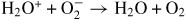
| (R39) | H2O+ + e → H2 + O(3P) | 1.40 × 10⁻⁷ | [30] |
| (R40) |
 |
1.73 × 10⁻⁷ | [30] |
| (R41) | H2O+ + O− → H2O + O(3P) | 4.00 × 10⁻⁷ | [30] |
| (R42) |
 |
4.00 × 10⁻⁷ | [30] |
| (R43) |
 |
1.20 × 10⁻⁹ | [62] |
| (R44) |
 |
1.50 × 10⁻⁹ | [62] |
| (R45) |
 |
2.00 × 10⁻¹⁰ | [63] |
| (R46) |
 |
3.00 × 10⁻¹⁰ | [63] |
| (R47) | O− + O2(a) → O3 + e | 3.00 × 10⁻¹⁰ | [63] |
| (R48) | O− + O(P) → O2 + e | 2.00 × 10⁻¹⁰ | [63] |
| (R49) | H− + H2O → OH− + H2 | 3.80 × 10⁻⁹ | [46] |
| (R50) | H− + H → H2 + e | 2.00 × 10⁻⁹ | [64] |
| (R51) | H− + O2 → HO2 + e | 1.20 × 10⁻⁹ | [65] |
| (R52) | OH− + H → H2O + e | 1.40 × 10⁻⁹ | [62] |
| (R53) | OH− + O(P) → HO2 + e | 2.00 × 10⁻⁹ | [65] |
Table 3. Considered reactions for neutral species.
| Reaction | A (cm3 s−1) | β | Ea (K) | Ref | |
|---|---|---|---|---|---|
| (R54) | N2(A1) + O2 → N2 + O(3P) + O(3P) | 1.70 × 10⁻¹² | 0 | 0 | [32] |
| (R55) | N2(A1) + O2 → N2 + O2(b) | 7.50 × 10⁻¹³ | 0 | 0 | [32] |
| (R56) | N2(A1) + O2 → N2O + O2(P) | 7.80 × 10⁻¹² | 0 | 0 | [66] |
| (R57) | N2(A1) + N2(A1) → N2 + N2(E) | 1.00 × 10⁻¹¹ | 0 | 0 | [35] |
| (R58) | N2(A1) + N2(A1) → N2 + N2(B) | 7.70 × 10⁻¹¹ | 0 | 0 | [32] |
| (R59) | N2(A1) + N2(A1) → N2 + N2(C) | 1.60 × 10⁻¹⁰ | 0 | 0 | [32] |
| (R60) | N2(A1) + O(3P) → N2 + O(1S) | 3.00 × 10⁻¹¹ | 0 | 0 | [46] |
| (R61) | N2(A1) + O(3P) → NO + N(2D) | 7.00 × 10⁻¹² | 0 | 0 | [35] |
| (R62) | N2(A1) + O(3P) → N2 + O(P) | 2.00 × 10⁻¹¹ | 0 | 0 | [35] |
| (R63) | N2(A1) + H → N2 + H | 2.10 × 10⁻¹⁰ | 0 | 0 | [35] |
| (R64) | N2(A1) + OH → N2 + OH | 1.00 × 10⁻¹⁰ | 0 | 0 | [35] |
| (R65) | N2(A1) + H2O → N2 + H + OH | 5.00 × 10⁻¹⁴ | 0 | 0 | [35] |
| (R66) | N2(A1) + NO → N2 + NO(A) | 6.90 × 10⁻¹¹ | 0 | 0 | [35] |
| (R67) | N2(A2) + N2 → N2(A1) + N2 | 1.00 × 10⁻¹¹ | 0 | 0 | [35] |
| (R68) | N2(A2) + O(P) → N2 + O(P) | 2.00 × 10⁻¹¹ | 0 | 0 | [35] |
| (R69) | N2(A2) + H → N2 + H | 2.10 × 10⁻¹⁰ | 0 | 0 | [35] |
| (R70) | N2(A2) + OH → N2 + OH | 1.00 × 10⁻¹⁰ | 0 | 0 | [35] |
| (R71) | N2(A2) + H2O → N2 + H + OH | 5.00 × 10⁻¹⁴ | 0 | 0 | [35] |
| (R72) | N2(A2) + NO → N2 + NO(A) | 6.90 × 10⁻¹¹ | 0 | 0 | [35] |
| (R73) | N2(A2) + O(P) → NO + N(S) | 7.00 × 10⁻¹² | 0 | 0 | [32] |
| (R74) | N2(B) + O2 → N2 + O(3P) + O(3P) | 3.00 × 10⁻¹⁰ | 0 | 0 | [32] |
| (R75) | N2(B) + N2 → N2(A1) + N2 | 1.00 × 10⁻¹¹ | 0 | 0 | [35] |
| (R76) | N2(B) → N2(A1) + hν | 1.50 × 10⁵ (s−1) | 0 | 0 | [32] |
| (R77) | N2(a) + O2 → N2 + O(3P) + O(3D) | 2.80 × 10⁻¹¹ | 0 | 0 | [32] |
| (R78) | N2(a) + N2 → N2(B) + N2 | 2.00 × 10⁻¹³ | 0 | 0 | [66] |
| (R79) | N2(a) + N2 → N2 + N2 | 2.00 × 10⁻¹³ | 0 | 0 | [35] |
| (R80) | N2(a) + H2 → N2 + H + H | 2.60 × 10⁻¹⁰ | 0 | 0 | [35] |
| (R81) | N2(a) + H2O → N2 + OH + H | 3.00 × 10⁻¹⁰ | 0 | 0 | [58] |
| (R82) | N2(a) + NO → N2 + N(4S) + O(3P) | 3.60 × 10⁻¹⁰ | 0 | 0 | [66] |
| (R83) | N2(C) + O2 → N2 + O(3P) + O(3P) | 2.50 × 10⁻¹⁰ | 0 | 0 | [32] |
| (R84) | N2(C) + N2 → N2(B) + N2 | 1.00 × 10⁻¹¹ | 0 | 0 | [32] |
| (R85) | N2(C) + N2 → N2(a) + N2 | 1.00 × 10⁻¹¹ | 0 | 0 | [35] |
| (R86) | N2(C) → N2(B) + hν | 2.80 × 10⁷ (s−1) | 0 | 0 | [35] |
| (R87) | N2(E) + N2 → N2(C) + N2 | 1.00 × 10⁻¹⁰ | 0 | 0 | [35] |
| (R88) |
 |
1.40 × 10⁷ (s−1) | 0 | 0 | [67] |
| (R89) | NO(A) → NO + hν | 5.10 × 10⁶ (s−1) | 0 | 0 | [35] |
| (R90) | N(2D) + O2 → NO + O(1D) | 9.70 × 10⁻¹² | 0 | −185 | [16] |
| (R91) | N(2D) + O2 → NO + O(3P) | 1.50 × 10⁻¹² | 0.5 | 0 | [66] |
| (R92) | N(2D) + NO → N2 + O(3P) | 1.80 × 10⁻¹⁰ | 0 | 0 | [68] |
| (R93) | N(2D) + N2 → N(4S) + N2 | 1.70 × 10⁻¹⁴ | 0 | 0 | [16] |
| (R94) | N(2D) + O(3P) → N(4S) + O(3P) | 3.30 × 10⁻¹² | 0 | −260 | [16] |
| (R95) | N(2D) + H2O → OH + NH | 4.00 × 10⁻¹¹ | 0 | 0 | [16] |
| (R96) | N(4S) + HO2 → NO + OH | 2.19 × 10⁻¹¹ | 0 | 0 | [69] |
| (R97) | N(4S) + NO → N2 + O(3P) | 3.51 × 10⁻¹¹ | 0 | 49.84 | [46] |
| (R98) | N(4S) + N(4S) + N2 → N2 + N2 | 1.38 × 10⁻³³ | 0 | 502.9 | [70] |
| (R99) | N(4S) + NO2 → NO + NO | 2.30 × 10⁻¹² | 0 | 0 | [46] |
| (R100) | N(4S) + NO2 → O(3P) + N2O | 5.80 × 10⁻¹² | 0 | 220 | [71] |
| (R101) | N(4S) + O2 → NO + O(P) | 4.47 × 10⁻¹² | 1 | 3270.2 | [72] |
| (R102) | O2(a) + N(S) → O(P) + NO | 2.00 × 10⁻¹⁴ | 0 | 0 | [71] |
| (R103) | O2(a) + O(P) → O(P) + O2 | 7.00 × 10⁻¹⁶ | 0 | 0 | [66] |
| (R104) | O2(a) + O2 → O2 + O2 | 2.20 × 10⁻¹⁸ | 0.8 | 0 | [73] |
| (R105) | O2(a) + N2 → O2 + N2 | 1.4 × 10⁻¹⁹ | 0 | 0 | [74] |
| (R106) | O2(a) + NO → O(P) + NO2 | 3.49 × 10⁻¹⁷ | 0 | 0 | [75] |
| (R107) | O2(a) + NO → NO + O2 | 2.50 × 10⁻¹¹ | 0 | 0 | [76] |
| (R108) | O2(b) + N2 → O2(a) + N2 | 2.10 × 10⁻¹⁵ | 0 | 0 | [77] |
| (R109) | O2(b) + O2 → O2(a) + O2 | 4.10 × 10⁻¹⁷ | 0 | 0 | [77] |
| (R110) | O2(b) + O(P) → O2 + O(P) | 8.00 × 10⁻¹⁴ | 0 | 0 | [77] |
| (R111) | O2(b) + H2O → O2 + H2O | 4.60 × 10⁻¹² | 0 | 0 | [77] |
| (R112) | O2(b) + O3 → O2(a) + O2(a) + O(P) | 1.80 × 10⁻¹¹ | 0 | 0 | [66] |
| (R113) | O2(b) + NO → O2(a) + NO | 4.00 × 10⁻¹⁴ | 0 | 0 | [66] |
| (R114) | O2(A) + O2 → O2(b) + O2(b) | 2.90 × 10⁻¹³ | 0 | 0 | [66] |
| (R115) | O2(A) + N2 → O2(b) + N2 | 3.00 × 10⁻¹³ | 0 | 0 | [66] |
| (R116) | O2(A) + O(P) → O2(b) + O(D) | 9.00 × 10⁻¹² | 0 | 0 | [66] |
| (R117) | O(3P) + O2 + N2 → O3 + N2 | 5.51 × 10⁻³⁴ | −2.6 | 0 | [77] |
| (R118) | O(3P) + O2 + O2 → O3 + O2 | 6.01 × 10⁻³⁴ | −2.6 | 0 | [77] |
| (R119) | O(3P) + O(3P) + N2 → O2 + N2 | 9.46 × 10⁻³⁴ | 0 | −484.7 | [78] |
| (R120) | O(3P) + O(3P) + O2 → O2 + O2 | 3.81 × 10⁻³³ | −0.63 | 0 | [79] |
| (R121) | O(3P) + N(4S) + N2 → NO + N2 | 6.89 × 10⁻³³ | 0 | −134.7 | [78] |
| (R122) | O(3P) + NO + N2 → NO2 + N2 | 1.03 × 10⁻³⁰ | −2.87 | −780.5 | [80] |
| (R123) | O(3P) + HO2 → OH + O2 | 2.70 × 10⁻¹¹ | 0 | −224 | [77] |
| (R124) | O(3P) + NO2 → O2 + NO | 5.50 × 10⁻¹² | 0 | 187.9 | [77] |
| (R125) | O(1D) + O2 → O(3P) + O2 | 3.12 × 10⁻¹¹ | 0 | −70 | [81] |
| (R126) | O(1D) + N2 → O(3P) + N2 | 2.10 × 10⁻¹¹ | 0 | −115 | [81] |
| (R127) | O(1D) + H2 → OH + H | 1.10 × 10⁻¹⁰ | 0 | 0 | [77] |
| (R128) | O(1D) + H2O → OH + OH | 2.2 × 10⁻¹⁰ | 0 | 0 | [77] |
| (R129) | O(1D) + H2O → H2 + O2 | 3.57 × 10⁻¹⁰ | 0 | 0 | [82] |
| (R130) | O(1D) + H2O2 → H2O + O2 | 5.20 × 10⁻¹⁰ | 0 | 0 | [77] |
| (R131) | O(1S) + H2O → O(P) + H2O | 3.00 × 10⁻¹⁰ | 0 | 0 | [83] |
| (R132) | O(1S) + H2O → OH + OH | 5.00 × 10⁻¹⁰ | 0 | 0 | [83] |
| (R133) | O(1S) + H2O → H2 + O2 | 5.00 × 10⁻¹⁰ | 0 | 0 | [83] |
| (R134) | O3 + H → OH + O2 | 1.40 × 10⁻¹⁰ | 0 | 480 | [74] |
| (R135) | O3 + NO → NO2 + O2 | 3.16 × 10⁻¹² | 0 | −1563 | [46] |
| (R136) | O3 + O(P) → O2 + O2 | 8.00 × 10⁻¹² | 0 | 2060 | [77] |
| (R137) | O3 + O(D) → O2 + O(P) + O(P) | 1.20 × 10⁻¹⁰ | 0 | 0 | [74] |
| (R138) | O3 + OH → HO2 + O2 | 1.70 × 10⁻¹² | 0 | 940 | [77] |
| (R139) | O3 + O3 → O2 + O(3P) + O3 | 7.16 × 10⁻¹⁰ | 0 | 11200 | [84] |
| (R140) | OH + OH + N2 → H2O2 + N2 | 6.90 × 10⁻³¹ | −0.8 | 0 | [77] |
| (R141) | OH + OH + O2 → H2O2 + O2 | 6.05 × 10⁻³¹ | −3 | 0 | [74] |
| (R142) | OH + OH + H2O → H2O2 + H2O | 1.54 × 10⁻³¹ | −2 | −183.6 | [86] |
| (R143) | OH + OH → H2O2 | 2.6 × 10⁻¹¹ | 0 | 0 | [77] |
| (R144) | OH + OH → H2O + O(3P) | 6.2 × 10⁻¹⁴ | 2.6 | −945 | [77] |
| (R145) | OH + H + N2 → H2O + N2 | 6.87 × 10⁻³¹ | −2 | 0 | [86] |
| (R146) | OH + H + H2O → H2O + H2O | 4.38 × 10⁻³¹ | −2 | 0 | [86] |
| (R147) | OH + HO2 → H2O + O2 | 4.8 × 10⁻¹¹ | 0 | −250 | [77] |
| (R148) | OH + N(4S) → NO + H | 3.80 × 10⁻¹¹ | 0 | −85.39 | [72] |
| (R149) | OH + O(3P) → O2 + H | 2.40 × 10⁻¹¹ | 0 | −110 | [77] |
| (R150) | OH + NO + N2 → HNO2 + N2 | 7.40 × 10⁻³¹ | −2.4 | 0 | [74] |
| (R151) | OH + NO + O2 → HNO2 + O2 | 7.40 × 10⁻³¹ | −2.4 | 0 | [74] |
| (R152) | OH + NO2 + N2 → HNO3 + N2 | 2.60 × 10⁻³⁰ | −2.9 | 0 | [74] |
| (R153) | OH + NO2 + O2 → HNO3 + O2 | 2.20 × 10⁻³⁰ | −2.9 | 0 | [74] |
| (R154) | HO2 + HO2 → H2O2 + O2 | 2.20 × 10⁻¹⁹ | 0 | −600.2 | [77] |
| (R155) | HO2 + NO → OH + NO2 | 3.60 × 10⁻¹² | 0 | −269.4 | [77] |
| (R156) | HO2 + HO2 + N2 → H2O2 + O2 + N2 | 1.90 × 10⁻³³ | 0 | −980 | [74] |
| (R157) | HO2 + HO2 + O2 → H2O2 + O2 + O2 | 1.90 × 10⁻³³ | 0 | −980 | [74] |
| (R158) | HO2 + NO2 → HNO2 + O2 | 1.20 × 10⁻¹³ | 0 | 0 | [85] |
| (R159) | H + HO2 → H2 + O2 | 1.75 × 10⁻¹⁰ | 0 | 1030 | [86] |
| (R160) | H + HO2 → H2O + O(3P) | 5.00 × 10⁻¹¹ | 0 | 866 | [87] |
| (R161) | H + HO2 → OH + OH | 7.40 × 10⁻¹⁰ | 0 | 700.0 | [86] |
| (R162) | H + O2 + O2 → HO2 + O2 | 5.94 × 10⁻³² | −1.0 | 0 | [46] |
| (R163) | H + O2 + N2 → HO2 + N2 | 5.94 × 10⁻³² | −1.0 | 0 | [46] |
Table 4. Effective electronic states of N2 and O2 considered in this simulation.
| Electronic state | Excitation energy (eV) | Effective state |
|---|---|---|
| N2(X, v = 0) | 0 | N2(X) |
 , v = 0 ... 4) , v = 0 ... 4) |
6.17 | N2(A1) |
|
, v = 5 ... 9) |
7.00 | N2(A2) |
| N2(B 3Πg) | 7.35 | N2(B) |
| N2(W 3Δu) | 7.36 | N2(B) |
|
, v > 10) |
7.80 | N2(B) |
 |
8.16 | N2(B) |
| N2
|
8.40 | N2(a) |
| N2(a 1Πg) | 8.55 | N2(a) |
| N2(w 1Δu) | 8.89 | N2(a) |
| N2(C3Πu) | 11.03 | N2(C) |
 |
11.88 | N2(E) |
 |
12.25 | N2(E) |
| O2(a 1Δg) | 0.977 | O2(a) |
O2
 |
1.627 | O2(b) |
| O2(c 1Σu) | 4.05 | O2(A) |
There are a large number of reaction pathways and rate constants that have been proposed to explain the relaxation kinetics from non-equilibrium conditions triggered by a discharge [45–44]; however, most of the rate constants are unknown or have only been estimated theoretically because of the difficulty of measuring such fast reactions. Therefore, we use only reliable reactions whose rate constants have been validated by direct measurements or indirect methods involving theoretical estimations and experimental results. For example, the quenching rate constant of N2
 by O2 is reliable since it has been directly measured and its validity has been confirmed in other papers [47, 48]. The rates of the recombination reactions of N2
are also reliable because the reaction kinetics of the N2 discharge, including some impurities, have been well modelled with the theoretically estimated recombination rates even though the rates were not fully measured [35, 37]. On the other hand, some detachment processes from negative ions that play important roles in discharge relaxation phenomena [62, 63, 65] are not well defined. The detachments induced by excited molecules of nitrogen, such as N2
and N2(B 3Πg), have not been clearly shown because the rate constants used in some studies on discharge modelling were taken from only one reference. Therefore, we use detachment reactions that have been investigated in more than one paper. For the other chemical reactions, we also attempted to find as many papers as possible with the help of the NIST database [49], and we chose the rate constants carefully. The vibration to vibration (VV) transitions and vibration to translation (VT) transitions are considered using our previously developed vibrational relaxation model [18]. However, they have no major effects in this simulation because the VV and VT transitions mainly occur several µs after the discharge [18].
by O2 is reliable since it has been directly measured and its validity has been confirmed in other papers [47, 48]. The rates of the recombination reactions of N2
are also reliable because the reaction kinetics of the N2 discharge, including some impurities, have been well modelled with the theoretically estimated recombination rates even though the rates were not fully measured [35, 37]. On the other hand, some detachment processes from negative ions that play important roles in discharge relaxation phenomena [62, 63, 65] are not well defined. The detachments induced by excited molecules of nitrogen, such as N2
and N2(B 3Πg), have not been clearly shown because the rate constants used in some studies on discharge modelling were taken from only one reference. Therefore, we use detachment reactions that have been investigated in more than one paper. For the other chemical reactions, we also attempted to find as many papers as possible with the help of the NIST database [49], and we chose the rate constants carefully. The vibration to vibration (VV) transitions and vibration to translation (VT) transitions are considered using our previously developed vibrational relaxation model [18]. However, they have no major effects in this simulation because the VV and VT transitions mainly occur several µs after the discharge [18].
Admittedly, the simplified reaction model does not describe all the kinetics triggered by the discharge. However, it is valid under limited conditions from the start of the discharge until 3 µs after the discharge pulse, as considered in this paper.
3. Results
3.1. Streamer discharge kinetics under humid-air conditions
Figure 3 shows the spatial distribution of discharge light emission obtained from the optical emission of the second positive system (SPS) of N2: C 3Πu → B 3Πg, whose intensity is proportional to the N2(C 3Πu) density. The numerically calculated SPS emission in the space r = (r, z) is spatially integrated along the line of sight. In addition, it is temporally integrated over 2 ns. Therefore, we calculate the time-integrated space-averaged optical emission [50, 51]. The primary streamer is formed near the anode tip and starts to propagate towards the plane cathode, as shown in figure 3. When the streamer head arrives at the plane cathode, the secondary streamer starts to extend. These characteristics of an atmospheric-pressure streamer discharge have been confirmed elsewhere in both experiments and simulations [10, 27, 52]. The light emission in humid air is similar to that in dry air. It is known that the changes in the spatial distribution and the time variation of the discharge emission depend on the gas composition and the shape of the applied pulsed voltage [52, 53]. Although the dependence of humidity on the discharge emission has not been clearly shown experimentally, the effect is estimated to be small from our simulated results. Figure 4(a) shows the axial distribution of the reduced electric field at several different times. The reduced electric field, E/N, is approximately 800 Td (1 Td = 10−17 V cm2) at the streamer head and it is almost constant when the streamer propagates to the plane cathode. However, the velocity of the streamer head and the reduced electric field in the streamer channel increase during its propagation through the gap. In our simulation, we confirmed that the propagation velocity of the streamer head and the reduced electric field in the streamer channel depend on the rate of increase in the applied pulsed voltage. The development of a reduced electric field in the primary streamer in humid air is not significantly different from that in dry air, obtained in our previous paper [10], because the ionization and photoionization rate coefficients are not changed for an admixture containing a few per cent of H2O in atmospheric-pressure air. However, the axial distribution of the reduced electric field in the secondary streamer is slightly different in dry and humid air, as shown in figure 4(b). The reduced electric field in the secondary streamer, which is known to be determined by the balance between the rates of ionization and attachment [10, 54], slightly increases with humidity. This slight increase is caused by the electronegative character of H2O. Figure 5 shows the total ionization and attachment rates in dry and humid air. The electron attachment reaction H2O + e → H− + OH causes the slight shift of the equilibrium point between the total ionization and attachment rates.
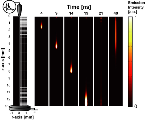
Figure 3. Calculated spatial distribution of discharge light emission at each time in H2O(2%)/air mixtures. The applied voltage is 28 kV.
Download figure:
Standard image High-resolution image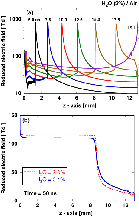
Figure 4. Axial distributions of reduced electric field (a) at various times during primary streamer propagation and (b) that at t = 50 ns when the secondary streamer appears. The applied voltage is 28 kV.
Download figure:
Standard image High-resolution image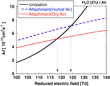
Figure 5. Dependence on the reduced electric field, E/N, of the rates of the ionization and attachment reactions in dry and humid air. k is the sum of rates of ionization and attachment reactions and δ is the fraction of nitrogen, oxygen or water in the mixture.
Download figure:
Standard image High-resolution image3.2. Comparison with experimental data
Figure 6 shows the simulated axial distribution of the OH radical density at t = 3 µs after the discharge pulse has elapsed. This result indicates that a large number of OH radicals as well as O and N radicals are produced near the anode tip [10]. Compared with our previous experimental results [19, 55], the simulated axial distribution of OH in figure 6 is in good qualitative agreement. However, the simulated axial distribution of OH radicals has a stepwise change in density around the edge of the secondary streamer head, whereas the experimentally measured OH radical density decreases exponentially from the point anode to the plane cathode along the discharge axis. This is because the simulated axial distribution of the reduced electric field in the secondary streamer changes in a stepwise manner at the secondary streamer tip, as shown in figure 4(b). This stepwise distribution has also been reported in a previous paper [27] and is theoretically well defined [31]. However, our previous experimental results indicate different characteristics. We previously measured the axial distributions of O [56], N [57], and OH [19, 55] radical densities and showed that these radical densities decrease exponentially from the point anode to the plane cathode. For these experiments, the limitations of the laser-induced fluorescence method used make measuring a stepwise shape around the edge of the secondary streamer head, as shown in figure 6, difficult because of experimental inaccuracies. Therefore, it is difficult to distinguish whether the difference is merely an error caused by the experiment itself, or an error caused by a physical phenomenon not considered in our simulation.
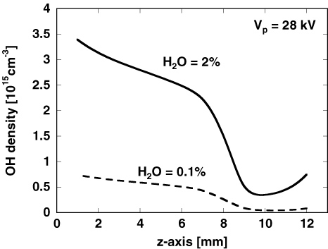
Figure 6. Axial distribution of OH radical density at t = 3 µs. The applied voltage is 28 kV.
Download figure:
Standard image High-resolution imageThe number of OH radicals produced in a single discharge pulse is simulated as shown in figure 7. Then, the effect of humidity on the number of OH radicals generated is compared with the experimental results [19]. Figure 7 indicates that the number of OH radicals produced by the discharge is saturated with increasing water vapour, and the simulation result is qualitatively consistent with the experiments except for a difference in the total number of OH radicals within a factor of 2. The mechanism of OH radical production is discussed in detail in the following section.

Figure 7. Total number of OH radicals at t = 3 µs as a function of H2O concentration. Experimental values were measured in our previous work [19].
Download figure:
Standard image High-resolution image3.3. Mechanism of OH radical production
The temporal behaviour of OH density in the rectangular section indicated in figure 8(a) is plotted in figure 9. The observation volume is set at z = 3 mm below the point anode, where the reactivity is high in the secondary streamer channel. Figures 8(b) and (c), respectively, show the temporal variation of the reduced electric field and electron density at the observation volume for z = 3 mm. These figures show how electrons are produced in large numbers in the primary streamer and that the number of electrons decreases in the secondary streamer, concomitant with a significant decrease in the reduced electric field, E/N, as explained in our previous paper [10]. Figure 9 shows the time variation of the OH radical density with H2O concentration at z = 3 mm, which is compared with the time variation in figures 8(b) and (c). From the comparison among figure 8(b) (E/N), figure 8(c) (electrons) and figure 9 (OH radicals), it is confirmed that the OH radicals are mainly produced in the secondary streamer and decrease in number after the discharge in two phases, labelled (i) and (ii). In particular, the rate of decrease in the second phase is accelerated with increasing humidity. This strong dependence of the decrease in OH radical density on humidity can explain the saturation of the number of OH radicals shown in figure 7. The detailed behaviour of OH radicals is explained in figure 10(a), which shows the time variation of the production and loss rates for each of the reactions leading to the formation of OH radicals as follows.

Figure 8. (a) Spatial distribution of O radical density at time t = 200 ns in H2O(2%)/O2/N2. Time evolution of (b) reduced electric field and (c) electron density at z = 3 mm. The applied voltage is 28 kV.
Download figure:
Standard image High-resolution image
Figure 9. Temporal variation of OH density at z = 3 mm. (i) denotes the first decay caused by processes of 'OH cycle' and (ii) denotes the second decay caused by processes of 'OH recombination'.
Download figure:
Standard image High-resolution image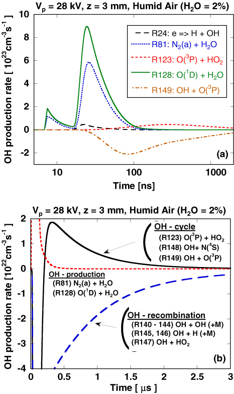
Figure 10. (a) Production rates for OH at z = 3 mm in H2O(2%)/O2/N2 mixture and (b) roles of each reaction in OH-production and loss processes.
Download figure:
Standard image High-resolution imageFirstly, the mechanism of OH radical production is discussed. From the results in figure 10(a), OH radicals are mainly produced by the dissociation reactions of O(1D) + H2O and N2(a) + H2O in the secondary streamer. Electron dissociation reactions such as e + H2O contribute less to OH radical production because the cross sections of these direct dissociation processes are low in the energy range of the secondary streamer compared with those of O(1D) and N2(a), as shown in figure 1. Although the dissociation of the reaction of O(1D) + H2O has been considered as one of the major pathways for OH radical production, the contribution of N2(a) to OH-production has not been discussed before. Therefore, its validity should be discussed here. Fresnet et al [35] first suggested the importance of the reaction of N2(a) + H2O. They concluded that the decrease in the decomposition rate of NO with the increase in humidity in an atmospheric-pressure photo-triggered discharge is caused by the quenching reaction of N2(a) by H2O because N2(a) plays the main part in the NO removal process. In addition, they measured the rate coefficient of the reaction of N2(a) + H2O indirectly from the temporal change in N2(a) and NO densities under several humid-air conditions. However, branching ratio of the reaction of N2(a) + H2O is unknown. Magne et al [58] and Aleksandrov et al [59] assumed that the branching ratio of N2(a) + H2O → N2 + O + OH is 1.0 in their plasma chemical reaction model and obtained good agreement between experimental and simulation results, although they did not pay sufficient attention to the branching reactions of N2(a) + H2O. In this work, we used the rate coefficients of N2(a) + H2O measured by Fresnet et al [35] and assumed the branching ratio to be 1.0, similarly to Magne et al [58] and Aleksandrov et al [59].
Next, the decrease in the number of OH radicals is discussed. The number of OH radicals produced in the secondary streamer rapidly decreases in two phases. The first decay (see (i) in figure 9) is caused by the reaction with O(3P), as shown in figure 10(a). The rate of OH-production by O(1D) and the rate of OH loss by O(3P) are similar in the discharge phase since similar amounts of O(1D) and O(3P) are produced by the direct dissociation process or dissociations by N2(A, B, C). However, the produced O(1D) are rapidly quenched by several species such as O2, N2 and H2O. Therefore, OH radicals are destroyed just after the discharge by the reaction with O(3P), producing H + O2. In figure 9, we can observe a temporal plateau of the OH radical density after the first decay and the subsequent second decay (see (ii) in figure 9). This phenomenon can be explained as follows using figure 10(b).
Figure 10(b) shows the time variation of the rates of reactions in three reaction processes: 'OH-production', 'OH-cycle' and 'OH-recombination', as shown in table 5. The rates of reactions in the OH-cycle change considerably from negative to positive at approximately 0.2–0.3 µs because the OH-cycle includes the OH-production reaction (R123) and (R161), and the OH loss reactions (R148) and (R149). The first negative rate in the OH-cycle is caused by the loss reactions (R148) and (R149) and the effect of the production reactions (R123) and (R161) emerges with increasing HO2, which is mainly produced by the reactions (R162) and (R163) through H radicals formed by the reactions (R148) and (R149). This is why we call this process the OH-cycle. The OH-cycle results in the first decrease in OH density (i) and the subsequent plateau phase between (i) and (ii), as shown in figure 9.
Table 5. Group of reactions arranged for the role of OH behaviour.
| OH-production | |
| (R81) | N2(a) + H2O → N2 + H + OH |
| (R128) | O(1D) + H2O → 2OH |
| OH-cycle | |
| (R123) | O(3P) + HO2 → OH + O2 |
| (R148) | OH + N(4S) → NO + H |
| (R149) | OH + O(3P) → O2 + H |
| (R161) | H + HO2 → 2OH |
| (R162) | H + O2 + O2 → HO2 + O2 |
| (R163) | H + O2 + N2 → HO2 + N2 |
| OH-recombination | |
| (R140) | OH + OH + N2 → H2O2 + N2 |
| (R141) | OH + OH + O2 → H2O2 + O2 |
| (R142) | OH + OH + H2O → H2O2 + H2O |
| (R143) | OH + OH → H2O2 |
| (R144) | OH + OH → H2O + O(3P) |
| (R145) | OH + H + N2 → H2O + N2 |
| (R146) | OH + H + H2O → 2H2O |
| (R147) | OH + HO2 → H2O + O2 |
The second decrease in OH density (ii) is explained as follows. From the results in figure 10(b), the decay of (ii) is caused by an OH-recombination process. The OH-recombination includes a number of OH loss processes involving the recombination reactions (R140)–(R144) or reactions with water-related radicals such as HO2 and H (R145)–(R147). Therefore, the rate of OH-recombination increases with the square of the water concentration. The OH-recombination allows us to interpret the decay of (ii) in figure 10(b) and the saturation of the experimentally obtained number of OH radicals in figure 7.
Figure 11 shows the flow of OH-production by the atmospheric-pressure streamer discharge. OH radicals are mainly produced by the reactions of N2(a) and O(1D) with H2O and are transformed into H2O or H2O2 via several recombination reactions with water-related radicals.

Figure 11. Schematic of OH radical production and loss processes.
Download figure:
Standard image High-resolution image
Under the present discharge conditions, we obtained OH-production pathways similar to that in figure 11. However, the pathways might be different under different conditions. For example, under the repetitive discharge conditions with a frequency of over 1 kHz, the gas temperature in the discharge volume might increase mainly by the vibrational relaxation phenomenon [18]. The recombination reactions in figure 11 have negative temperature coefficients, and therefore the rate of decrease of OH density after the discharge might be slower than that considered in this paper. To simulate the increase in the gas temperature accurately, the fast gas heating model [32] and the vibrational relaxation model [18] should be coupled with the Navier–Stokes equations to consider the effect of compressibility [30, 34]. In addition, the rate of current relaxation simulated by the extended Morrow and Sato equation [29], as shown in figure 2, is slightly faster than that observed experimentally [14]. The rates of the electron attachment and detachment reactions, which are considered to be important for current relaxation, need to be examined carefully. Moreover, complex ions may also affect the rate of current relaxation. Complex ions were ignored in this simulation because we were able to reproduce the primary and secondary streamers well without them. It may be necessary to evaluate the effect of complex ions on the production of radicals for a more precise simulation.
4. Conclusion
In this paper, the mechanisms of OH radical formation in an atmospheric-pressure streamer discharge were discussed. The axial distribution of OH radical density and the effect of humidity on OH-production were qualitatively reproduced in our two-dimensional streamer discharge model. The following conclusions were drawn from this study.
- The OH radicals are mainly produced in the secondary streamer, and the dissociation of H2O by O(1D) and N2(a) is predominant in the production of OH. The density of OH radicals measured in humid nitrogen can be explained by considering the effect of OH-production processes related to excited nitrogen species, although the dissociation reaction via N2(a) needs further consideration.
- After the production of OH radicals, the OH radical density is rapidly decreased by the reactions of OH with O(3P). However, the H radicals resulting from the OH + O(3P) and OH + N(4S) reactions are transformed into HO2, then the HO2 produces OH again by the reaction with O(3P).
- Once the above 'OH-cycle' reactions reach quasi-equilibrium, the 'OH-recombination' reaction comes into play. As a result, the produced OH changes into H2O or H2O2 by recombination reactions with water-related radicals. These simulation results provide a good interpretation of OH radical production in N2/O2/H2O mixtures.
Acknowledgments
This work was supported by Grant-in-Aid for Japan Society for the Promotion of Science (JSPS) Fellows.