
Abstract
The effective Townsend ionization coefficient in nitrogen–oxygen mixtures at various pressures is determined. In addition to the commonly accepted difference of the ionization and the attachment coefficients, α and η, respectively, the electron detachment from the negative ions created by the avalanche itself is taken into account. This leads to non-zero effective ionization rate below the threshold field corresponding to α − η = 0.
Export citation and abstract BibTeX RIS
1. Introduction
It is generally accepted that inception of a gas discharge starts with the appearance of a first free electron in the gap. Depending on the conditions, such electrons can be emitted from a surface or can appear by detachment from a negative ion (
 ,
,
 ,
,
![${\rm O}_z^- \cdot [{\rm H}_2{\rm O}]_n$](https://content.cld.iop.org/journals/0022-3727/46/15/155201/revision1/jphysd448859ieqn003.gif) , etc). At high pressures, it is the detachment process which typically creates free electrons in the gap. Background pre-ionization is produced by 'natural' ionizing radiation (cosmic rays, ingested radioactivity, etc) or can remain from previous discharges in repetitively pulsed mode [1].
, etc). At high pressures, it is the detachment process which typically creates free electrons in the gap. Background pre-ionization is produced by 'natural' ionizing radiation (cosmic rays, ingested radioactivity, etc) or can remain from previous discharges in repetitively pulsed mode [1].
A Townsend avalanche usually develops from the initiating electron. The total number of electrons in the avalanche initiated at x = 0 from number N0 of initial electrons (often N0 = 1) is described by

where the ionization integral K(x) is defined as

Here αeff is known as effective Townsend's ionization coefficient, defined as the number of electrons produced by an electron per unit length of path in the direction of the field. In general, the effective ionization coefficient can be determined from the ionization coefficient α and the attachment coefficient η as

In spite of a very long history, the calculation of ionization integral (2) in air requires care due to significant discrepancies in the net ionization coefficient αeff measured by different authors [2].
An alternative kinetic approach deals with the calculation of the electron energy distribution function based on a detailed description of elementary processes in gas. The main processes which take place in non-excited nitrogen–oxygen mixtures are the motion of charged species (drift of electrons in electric field), collisional ionization by electron impact (4) and (5) and attachment (6) and (7):


where M = {N2, O2}. The relations which link the ionization and attachment Townsend coefficients α, η and the constant rates ki of corresponding reactions, the electron drift velocity
 and gas densities are


where [N2], [O2] and [M] are the densities of nitrogen, oxygen and the total gas density, respectively.
In this work, electron swarm parameters and reaction rates are calculated using the online version of the BOLSIG+ solver [3] and the SIGLO database [4] for electron–neutral scattering cross sections. Within this approach, electron swarm parameters and reaction rates are functions of the reduced electric field E/N, which is the ratio of the applied electric field E and gas density N(N = [M]).
Similarly, we can define partial Townsend coefficients corresponding to a specific process. Calculated in this way the attachment coefficients are


Their reduced values, i.e. obtained by division with the gas density, are plotted in figure 1 for oxygen and air at atmospheric pressure and gas temperature Tgas = 300 K.
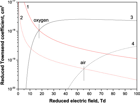
Figure 1. Reduced attachment Townsend coefficients η7 (1,2) and η6 (3,4). Oxygen (1,3) and air (2,4) at 1 bar, 300 K. The dominant negative ion is
 at low fields and O− at high fields.
Download figure:
Standard imageAs follows from the figure, the three-body attachment (7) dominates over the two-body attachment (6) at low electric fields (below 20 Td in oxygen and 55 Td in air at atmospheric pressure). Its contribution at lower pressures is less important.
Detachment of electrons from negative ions created by the avalanche can also be the source of electrons, especially at low electric fields. The presence of an after-current caused by delayed electrons has been demonstrated first in oxygen and air at low pressures [5] and later confirmed for atmospheric-pressure air [6, 7]. It was assumed that the delayed electrons arrive due to detachment from negative ions. Available experimental measurements of electron attachment–detachment processes in oxygen and air are summarized in [8].
Note, the associative detachment from O−,
and
 ions in collisions with atomic oxygen or electronically excited molecules is known to be very efficient [9]. This case requires elevated densities of the corresponding excited species and radicals and will not be considered in this paper.
2. Collisional detachment of electrons from negative ions
2.1. Ion temperature at elevated fields
Detachment of electrons from negative ions at elevated electric fields mainly occurs in collisions of the ions with neutral molecules. The translational temperature of ions differs from the gas temperature due to the drift of ions in the applied electric field.
The ion drift velocity vion can be expressed through the reduced mobility, μ N, and the reduced electric field, E/N, as

The mobility of ions is often assumed to be constant; however, it can significantly vary with electric field. In this work we are interested in the ion behaviour near the breakdown threshold; the values of ion mobility have been taken from [10] at E/N = 100 Td and presented in table 1.
Table 1. Reduced mobility μ N in (m V s)−1 of selected negative ions in pure oxygen and dry air at E/N = 100 Td retrieved from [10].
| O− |
|
|
 |
|
|---|---|---|---|---|
| Oxygen | 1.2 × 10²² | 5.0 × 10²¹ | 8.1 × 10²¹ | — |
| Air | 1.2 × 10²² | 7.1 × 10²¹ | 7.6 × 10²¹ | 6.6 × 10²¹ (in N2) |
An analytical expression for the mean translational energy of ions Eion has been originally derived by Wannier under the assumption of a constant mean free time between collisions [11, 12]

where mion and mgas are the masses of the ions and gas molecules, vion is the ion drift velocity. Here and below, temperatures are considered in energy units, i.e. multiplied by the Boltzmann constant.
Relation (13) has been obtained for elastic collisions without considering charge-exchange collisions between ions and gas. This result is hardly applicable to the drift of ions in parent gas at elevated fields where these types of collisions are known to be dominant.
Fahr and Miller [13, 14] investigated the drift motion of ions when charge-exchange collisions dominate and derived velocity distributions for the extreme cases of very small (qeEλ ≪ Tgas) and very high reduced electric fields (qeEλ ≫ Tgas), where λ is the mean free path for charge exchange. At high E/N the ions' thermal motion becomes negligible compared with the drift. In this case, the velocity distribution f(vz) in field direction z is given by
where θz = qeEλ is the effective ion temperature in field direction; the ion velocity is limited by vz ⩾ 0. The drift velocity can be deduced from the ion velocity distribution as
The latter allows one to obtain the ion effective temperature in field direction from the drift velocity

Note that the last term related to gas temperature Tgas is artificially added to the result in order to get θz = Tgas limit at zero field. This allows one to use the relation (16) for the entire range of ion energies with a reasonable accuracy.
Similar to drift velocity, the ion mean translation energy expressed in terms of the drift velocity becomes

that is approximately 20–25% lower than Wannier's original relation (13).
The calculated translation energies of the most important negative ions in nitrogen–oxygen mixtures (O−,
,
and
 are presented in figure 2. The obtained values for
in pure oxygen correspond to those obtained using direct Monte-Carlo modelling of ion transport [15]. Another example of good agreement has been demonstrated in [16] for argon. These results encourage us to extend this approach to other ions and gases.
are presented in figure 2. The obtained values for
in pure oxygen correspond to those obtained using direct Monte-Carlo modelling of ion transport [15]. Another example of good agreement has been demonstrated in [16] for argon. These results encourage us to extend this approach to other ions and gases.

Figure 2. Ion mean translation energy Eion (17) as a function of reduced electric field in oxygen and dry air. Symbols are the results of direct Monte-Carlo simulation [15].
Download figure:
Standard imageIt is important to note that the relation θz = 2 Eion between the effective ion temperature (16) and the mean energy (17) remarkably differs from the well-known ideal gas case Tion = 2/3 Eion.
2.2. Ion–neutral reaction constant rate
Ion velocity distribution (14) allows us to calculate the constant rate k for a process with known cross section σ( ) as
) as

For an inelastic process with the energy threshold Δ (activation energy), assuming linear variation of the corresponding cross section near the threshold and low gas temperatures (θz ≫ Tgas), the following Arrhenius form becomes valid

Here k0 is energy-independent part of the reaction constant rate and θz is the ion effective temperature in field direction (16).
Strictly speaking, the use of reaction rate (19) is limited by relatively high electric fields when θz ≫ Tgas. A commonly used approach (see, for example, [9, 17]) recommends to use instead of θz the effective temperature of ion–neutral collisions Teff defined as

This relation, however, assumes isotropic distribution of the velocities of colliding species in space and its use for ion–neutral collisions is questionable. In fact, the motion of ions in parent gas exhibits significant anisotropy (14) with the dominant motion in the field direction. To adapt the above-mentioned relation, one could assume Tion ≃ 2θz, that gives Teff ≃ θz in the case of similar ion and neutral masses. This allows us to use the ion effective temperature in the field direction (16) for ion–neutral reaction rate approximations (19).
2.3. Detachment in oxygen
The main negative ion created in oxygen at elevated fields (above 20 Td at atmospheric pressure, figure 1) is O−. However, it is generally accepted that detachment of electrons in pure oxygen occurs mainly in collisions of
ions with O2 molecules

and the detachment rate from O− ions in pure oxygen is almost negligible due to the fast reaction of charge transfer to molecules

For the following analysis, we approximate the constant rate of reactions according to (19)
for (21), which matches the experiment [23] and the detachment rate calculated on the basis of the statistical approach [24] fairly well with the parameters
 and Δ21 presented in table 2.
Table 2. Arrhenius approximation of reaction constant rates k = k0exp(−Δ/θ) (21), (22), (27) and k = k0 exp(−θ/Δ) (25).
| Proc. | k0 | Δ (eV) |
|
|---|---|---|---|
 |
(21) | (1.22 ± 0.07) × 10−11 cm3 s−1 | 0.78 ± 0.03 |
 |
(22) | (6.9 ± 0.6) × 10−11 cm3 s−1 | 1.40 ± 0.14 |
| O− + N2 ⇒ N2O + e | (27) | (1.16 ± 0.05) × 10−12 cm3 s−1 | 0.076 ± 0.005 |
 |
(25) | (1.3 ± 0.2) × 10−30 cm6 s−1 | 0.16 ± 0.05 |
Similarly, fitting the experiments [18–20, 25, 26], the charge transfer reaction rate (22) can be approximated by

Experimentally measured rates of both processes and corresponding Arrhenius rates are presented in figure 4. The fitted parameters are summarized in table 2 and will be used for the determination of detachment rate in air.
Detachment from heavy ions, such as
, is hardly observed in oxygen. This ion is easily created at low fields in the following three-body associative reaction

when the translation energy of ions is not sufficient for effective collisional detachment (see table 1 and figure 2) and, thus, it can be considered as a stable negative ion. At higher fields,
is not created due to a fast charge transfer reaction similar to (22).
Experimentally measured reaction rate of (25) from [18–22] and its fitted approximation (table 2)

are both presented in figure 3.
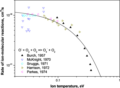
Figure 3. Reaction rate of three-body
production (25). Symbols are experimental measurements [18–22] and line is the approximation of k25 (26).
Download figure:
Standard image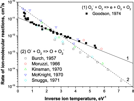
Figure 4. Arrhenius plot of the ion–molecular reaction rates in oxygen. Symbols are experimental measurements [18–20, 23, 25, 26] and lines are the Arrhenius approximations: 1—k21 (23) and 2—k22 (24).
Download figure:
Standard image2.4. Detachment in dry air
The constant rates k21 (23) and k22 (24) obtained for pure oxygen can be used for description of processes in air using corresponding mobilities for determination of ion temperatures. The detachment reaction rate obtained in this way for air and oxygen is presented in figure 5. As follows from the Figure, the detachment rate in air remains remarkably higher in the entire range of electric fields. It follows from the higher mobility (table 1) and, correspondingly, the higher energy of
ions in air (figure 2).

Figure 5. Detachment reaction rate k21 (23) from
ions in air and oxygen versus reduced electric field.
Download figure:
Standard imageAn extra process, namely associative detachment, has to be considered in air:

It is an exothermic reaction and it contributes to the detachment balance already at low electric fields. This process, however, has a barrier of 0.1–0.2 eV as was pointed out in [27]. In this study, the following approximation was used to fit the measurements [27, 28]

Experimentally measured and approximated constant rates for reactions (21), (22) and (27) are summarized in figure 6. Corresponding constant rates are taken according to (23), (24) and (28) and the corresponding ion temperatures (16) in air.
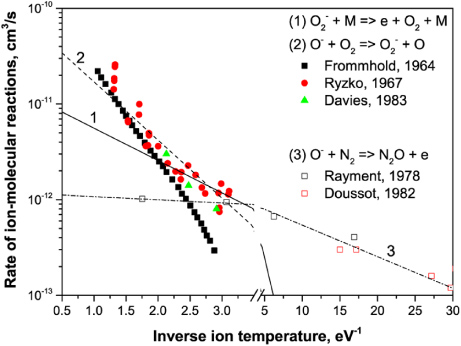
Figure 6. Arrhenius plot of the ion–molecular reaction rates in dry air. Symbols are experimental measurements [27–31] and lines are the Arrhenius approximations: 1—k21 (23), 2—k22 (24) and 3—k27 (28).
Download figure:
Standard imageThe detachment rate from
ions (23) demonstrates fairly good agreement with measurements for E/N = 100–150 Td that corresponds to 1/θ = 2.5–5.0 eV−1 inverse temperature range. As follows from the figure, experimental measurements at higher fields E/N = 150–200 Td (below 2.5 eV−1) are in good agreement with the charge transfer reaction (22) which is the dominant process for O− ions.
The reaction rates for O− ions in air are presented in figure 7 as a function of reduced electric field. Three regions with different detachment mechanisms can be identified using figures 1 and 7. For low electric fields (E/N < 50 Td), the most important process leading to electron detachment is the associative detachment on nitrogen molecules (27), as expected. However, the dominant negative ion at atmospheric pressure at low fields is
which hardly contributes to detachment at these fields.

Figure 7. Ion–neutral reaction rates for O− ions in air versus reduced electric field: k22 (24), k27 (28) and k = k25 [M] (26) for three different pressures (Tgas = 300 K). [M] is the total gas density.
Download figure:
Standard imageFor E/N in the range 50–100 Td, the dominant ion is O− and the electron detachment (27) starts contributing to the overall production of electrons (figure 7). This process, however, remains relatively weak at elevated pressures in comparison with the three-body charge transfer to ozone (25).
At higher fields, E/N > 100 Td, the charge transfer (22) with consequent collisional detachment (21) is the dominant process. This can be schematically summarized in the following diagram:
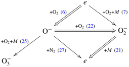
Under conditions of constant electric field,
can be considered as a stable negative ion because its formation occurs only at low electric fields (figure 3). At higher fields (E/N > 70 Td), these ions convert rapidly into O− and contribute to the main chain of electron detachment at high fields (double-line path).
3. Effective ionization coefficient
Similar to the theoretical model proposed by Verhaart and van der Laan [6], four species have to be involved for the determination of effective ionization coefficient: electrons (index e), positive ions (p), unstable negative ions (nu) and stable negative ions (ns). Compared with stable negative ions
, the unstable negative ions O− and
have a relatively short lifetime and are able either to release their electrons, or to be converted (stabilized/charge transferred) into stable ones within the ion transit time [6]. The development of avalanche can then be expressed as


To determine the effective ionization coefficient
 , we resolve this system of equations assuming the electron solution in the following form:

Substituting the latter into the system of equations and limiting our interest to
 , we obtain

It is easy to check that
 . Note that formula (34) for the effective ionization coefficient is similar to those derived in [6] and can be reduced under certain simplifications from the general expression obtained in [2].
3.1. Oxygen
In the relatively simply case of an avalanche development in oxygen, we can use the following reduced set of processes—ionization (5), two-body dissociative attachment (6) and collisional detachment (21) assuming that the ion conversion
 occurs much faster than the detachment (according to figure 4, the latter is correct for ion temperatures above approximately 0.3 eV). The following partial Townsend coefficients can be used:

The resulting effective ionization coefficient, as well as the ionization and attachment coefficients, in oxygen are presented in figure 8. The most pronounced additional production of elections due to the effect of electron detachment occurs in the range of low electric fields. At low fields, the attachment losses dominate over ionization and the commonly used net ionization coefficient αeff is negative; that means no avalanche can develop at electric fields below 125 Td. In contrast,
in considering electron detachment goes to zero at considerably lower fields, i.e. avalanches can develop in under-critical electric fields where α − η < 0.

Figure 8. Reduced ionization α/N (8) and attachment η/N (9) coefficients in oxygen together with their difference αeff/N = (α − η)/N and calculated effective coefficient
 (34) for three different pressures (Tgas = 300 K). Symbols are the measurement [32] and review [2].
Download figure:
Standard imageEffective ionization coefficients in different gases, including oxygen, have been measured numerously. For instance, the measured results [32] and the review of six independent publications [2] are presented in the figure 8 for the range 100–190 Td. As follows from comparison, the measured values agree fairly well with the value of net effective ionization coefficient obtained in the present study assuming the gas pressure below 1 bar (that is usually the case for drift-tube experiments [2]). The effect of electron detachment decreases when pressure increases. However, the difference between αeff and
remains remarkable even at pressures above 10 bar (figure 8).
3.2. Air
The same approach can be applied for air (more generally, for a nitrogen–oxygen mixture) substituting

The result obtained in this way and experimentally measured values of the effective ionization rates in air [2, 32, 33] are presented in figure 9. So, the approximation proposed in [33] is an analytic expression matching the experimental values of various authors for dry air and for air under controlled humidity conditions. The results of this approximation are in good agreement with the effective ionization rate αeff = α − η commonly accepted. At the same time, measurements [2, 32] give much higher values at lower electric fields and agree relatively well with the results of this work.
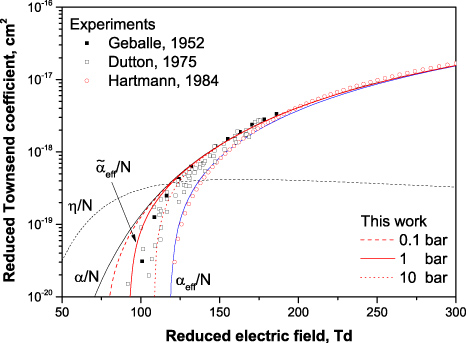
Figure 9. Reduced ionization α/N (8) and attachment η/N (9) coefficients in air together with their difference αeff/N = (α − η)/N and calculated effective coefficient
(34) for three different pressures (Tgas = 300 K). Symbols are the measurements [32] and data reviews [2, 33].
Download figure:
Standard imageIn spite of significant scattering of experimental points at low electric fields (below 150 Td) reported by different groups, the general trend remains the same. A systematic measurement of the reduced effective ionization rate in air is reported in [2] for the gas density range 10−19–10−20 cm−3 and the following fixed values of electric field: 101.5, 103.0 and 104.5 Td. These points and the results of current modelling are presented in figure 10. The maximum discrepancy between the both results reaches approximately two times at low densities and fields but it still remains below the typical uncertainty of experimental measurements at under-critical fields (see figure 9).
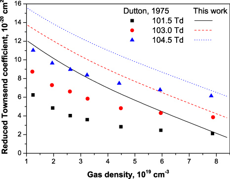
Figure 10. Reduced effective ionization coefficient
in air measured [2] (symbols) and calculated here (curves) for different gas densities at three fixed values of electric field.
Download figure:
Standard image4. Critical electric field
According to equation (34), the critical electric field (E/N)cr corresponding to zero ionization coefficient
 lies in the range α − η ⩽ 0. It is defined by the following condition:

The values of critical electric field calculated according to this relation are presented in figure 11 for oxygen and air as a function of gas pressure. According to the figure, the critical electric field varies significantly with the gas pressures (density) and even at elevated pressures remains remarkably lower than those given by the condition α − η = 0—approximately 125 Td in O2 and 120 Td in air.
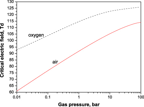
Figure 11. Critical electric field corresponding to zero net ionization (37) in oxygen and dry air as a function of gas pressure at Tgas = 300 K.
Download figure:
Standard image5. Detachment timescale
One of the simplifications made in this work is the assumption that the solution can be considered as quasi-steady which may be justified by a time scale separation. However, detachment of electrons does not occur instantaneously and it requires certain time that has to be compared with the characteristic time of the task under consideration. The detachment time, or inverse detachment frequency, can be estimated as

The values of the detachment time in oxygen and air under normal conditions calculated in this way are presented in figure 12. In oxygen, this time changes from nanoseconds at elevated fields (E/N > 250 Td) up to microseconds at lower fields (E/N < 100 Td). The detachment time in air, in turn, remains below 100 ns in the entire field range under this study. The latter value is in agreement with the experimentally registered duration of current pulses 200–800 ns near the threshold voltages of corona inception in air at atmospheric pressure [34].
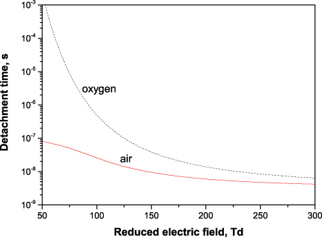
Figure 12. Electron detachment time from negative ions in oxygen and air, 1 bar, 300 K. The detachment time scales with the gas density as ∝ 1/N.
Download figure:
Standard imageNote that according to (38), the detachment time is proportional to the inverse gas density τdet ∝ 1/N and the contribution of detachment at lower densities (pressures) can be much less important than at higher gas densities (pressures).
6. Conclusions
The effective Townsend ionization constant is determined. In addition to the commonly accepted difference of the ionization and the attachment coefficients, α and η, respectively, the electron detachment from the negative ions created by the avalanche itself is taken into account. This leads to non-zero effective ionization rate below the threshold field corresponding to α − η = 0.
The corrected value of electric field corresponding to zero effective ionization rate is determined for oxygen and air. In spite of the decreasing role of detachment with pressure increase, its contribution remains remarkable up to pressures about 100 bar. The time lag appearing due to attachment–detachment delay increases in 1 bar oxygen from 10 ns at high fields up to 1 ms at 50 Td. Meanwhile, electron detachment in atmospheric-pressure air occurs at the time scale of 100 ns.
: Appendix
Reaction constant rates can be approximated for practical purposes according to (16) and (19) as a function of reduced electric field (figures 5 and 7)


Similarly, the following approximation for the effective ionization rate (34) can be used at 1 bar, 300 K (figures 8 and 9)
Here k is in cm3 s−1 (k25 in cm6 s−1), α/N is in cm2 and E/N is in Td (1 Td = 10−17 V cm2). The range of electric fields 50–300 Td is mainly considered in this paper.