


ABSTRACT
We present a new set of nonlinear, convective radial pulsation models for main-sequence stars computed assuming three metallicities: Z = 0.0001, 0.001, and 0.008. These chemical compositions bracket the metallicity of stellar systems hosting SX Phoenicis stars (SXPs, or pulsating Blue Stragglers), namely, Galactic globular clusters and nearby dwarf spheroidals. Stellar masses and luminosities of the pulsation models are based on alpha-enhanced evolutionary tracks from the BASTI website. We are able to define the topology of the instability strip (IS) and in turn the pulsation relations for the first four pulsation modes. We found that third overtones approach a stable nonlinear limit cycle. Predicted and empirical ISs agree quite well in the case of 49 SXPs belonging to ω Cen. We used theoretical period–luminosity (PL) relations in B and V bands to identify their pulsation mode. We assumed Z = 0.001 and Z = 0.008 as mean metallicities of SXPs in ω Cen. We found respectively 13–15 fundamental, 22–6 first-overtone, and 9–4 second-overtone modes. Five are unstable in the third-overtone mode only for Z = 0.001. Using the above mode identification and applying the proper mass-dependent PL relations, we found masses ranging from ∼1.0 to 1.2  (
( = 1.12,
 ) and from ∼1.2 to 1.5
  (
( = 1.33,
 ) for Z = 0.001 and 0.008, respectively. Our investigation supports the use of evolutionary tracks to estimate SXP masses. We will extend our analysis to higher helium content, which may have an impact on our understanding of the blue straggler stars formation scenario.
Export citation and abstract BibTeX RIS
1. INTRODUCTION
Blue straggler stars (BSSs) are bluer and brighter than the main-sequence (MS) turnoff (MSTO) stars. They define a sequence that in the optical color–magnitude diagram (CMD) can span more than 2 mag above the cluster MSTO. They mimic a younger stellar population with masses (M = 1–1.7  ; Shara et al. 1997; Gilliland et al. 1998; De Marco et al. 2005; Fiorentino et al. 2014) significantly larger than normal cluster stars (MSTO = 0.8–0.9
  ). For this reason they have been suggested to have originated from collision-induced mergers, most likely in dense stellar environments (Hills & Day 1976; Leonard 1989), or by mass exchange in primordial binary systems (McCrea 1964; Zinn & Searle 1976; Ferraro et al. 2006a, 2006b; Knigge et al. 2009). Both formation channels can possibly be active within the same cluster (Ferraro et al. 2009b; Xin et al. 2015). SX Phoenicis stars (SXPs) are pulsating BSSs (McNamara 2011, and references therein) that are observed both in old (globular clusters [GCs]) and intermediate-age (dwarf galaxies) stellar populations. SXPs are particularly important objects because their pulsation properties can provide a viable way to derive structural parameters of BSSs. In particular, the measure of the BSS mass is crucial since they have been recently used to define the so-called dynamical clock (Ferraro et al. 2012), an empirical tool able to rank GCs on the basis of their dynamical ages. Since the engine of such a clock is dynamical friction and since the dynamical friction directly depends on the object mass, an accurate determination of BSS masses is of paramount importance for the calibration.
SXPs have luminosity amplitudes ranging from a few hundredths to tenths of a magnitude, their periods are typically shorter than 0.1 days, and they can pulsate simultaneously in radial and nonradial modes. They have been identified in several stellar systems, not only in Galactic GCs but also in nearby dwarf irregulars (Small Magellanic Cloud, Large Magellanic Cloud, Soszynski 2002; Soszynski et al. 2003; Poleski et al. 2010; IC 1613 Irr, Bernard et al. 2010) and dwarf spheroidals (Fornax, Poretti et al. 2008; Carina, Mateo et al. 1998; Vivas & Mateo 2013). The improvement in the empirical scenario concerning SXPs was driven by the ongoing long-term photometric surveys. The mosaic CCD cameras available in ground-based 4–8 m class telescopes and the Advanced Camera for Surveys at the Hubble Space Telescope (HST) provided the opportunity to collect optical, multiband, time-series data of MSTO stars of both the old and the intermediate-age stellar populations in the quoted stellar systems. The main pros of SXPs when compared with other regular variables are their short periods; thus, SXPs can be identified even with data sets that only cover a few hours of observations. They are also ubiquitous: they have been identified in all the stellar systems investigated. The main con is that the luminosity amplitude is at most of the order of a few tenths. This means that very precise and accurate photometry down to the MSTO level is required.
The latter empirical evidence and the fact that their oscillations are a mix of radial and nonradial modes are the main reasons why the pulsation characterization (amplitudes, modes, mean magnitudes) of cluster SXPs is only available for a limited sample of objects. However, there is solid empirical evidence (McNamara 2011) that nonradial modes become less and less relevant as soon as the stars evolve off the zero-age MS. This means that the opportunity exists to use nonlinear convective radial models to constrain the pulsation properties of SXPs.
This is the second paper of a series (see Fiorentino et al. 2014) on a project aimed at developing a new theoretical framework for stellar oscillations in high-gravity variables. We undertook this project since we plan to use pulsation observables to constrain the intrinsic parameters of SXPs (and BSSs). In Paper I (Fiorentino et al. 2014) we provided the pulsation relations to estimate the mass of SXPs using the linear, radial models provided by Santolamazza et al. (2001). The above analysis concerning the pulsation masses of SXPs was based on the assumption that their pulsation mode can be constrained using the period–luminosity (PL) relations.
In this paper, we further improve our analysis constructing a new set of nonlinear, nonlocal, and time-dependent convective SXP models (see Section 2). This approach allows us to constrain the morphology of the instability strip (IS) for each assumed pulsation mode. We also describe the approach adopted to compute synthetic stellar populations and the pulsation relations (see Sections 2, 3, and 4). In Section 5 we applied the new theoretical framework to ω Centauri. The summary of this investigation, the further developments of the project, and a few final remarks are given in Section 6.
2. EVOLUTIONARY AND PULSATION MODELS
In this section we present the new SXP models. To select the input stellar parameters for the nonlinear pulsation computations, we considered the evolutionary tracks of the BASTI (A Bag of Stellar Tracks and Isochrones) database (http://basti.oa-teramo.inaf.it/index.html; see Pietrinferni et al. 2004, 2006, and references therein) for stellar masses ranging from 1.0 to 1.8  and three chemical compositions, namely, Z = 0.0001 (Fe/H = −2.62), Z = 0.001 (Fe/H = −1.62), and Z = 0.008 (Fe/H = −0.70). The adopted evolutionary tracks are shown in Figure 1 and correspond to the alpha-enhanced models (see Pietrinferni et al. 2006, for details). For each stellar mass and chemical composition, we evaluated the pulsation instability along the corresponding evolutionary track, varying the effective temperature with a step of 100 K and applying a nonlinear hydrodynamical code that includes a nonlocal time-dependent treatment of convection (see Stellingwerf 1982; Bono et al. 1999, 2002). All the input parameters are given in Table 1.
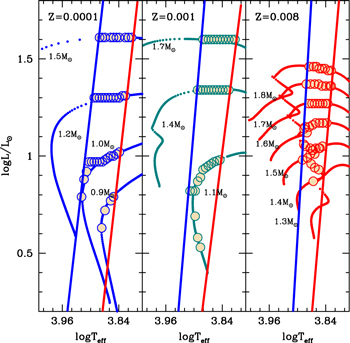
Figure 1. Portion of the Hertzsprung–Russell diagram where alpha-enhanced evolutionary tracks are shown from the BASTI website (Pietrinferni et al. 2004) for selected metallicity values that bracket values typical for Galactic GCs, e.g., Z = 0.0001 (blue), Z = 0.001 (teal), and Z = 0.008 (red). For each metallicity a mass range has been selected: 1.0, 1.2, and 1.5  for Z = 0.0001; 0.9, 1.1, 1.4, and 1.7
  for Z = 0.001; 1.4, 1.5, 1.6, 1.7, and 1.8
  for Z = 0.008. We also show the position in the CMD of the pulsation models (expanded dots) selected in order to roughly follow the evolutionary path. The blue and red edges derived by the pulsation instability are also shown.
Download figure:
Standard image High-resolution imageTable 1. Input Parameters for the Pulsation Models

|
Teff | Mode |

|

|
Teff | Mode |

|

|
Teff | Mode |

|
|---|---|---|---|---|---|---|---|---|---|---|---|
| Z = 0.0001, Y = 0.24 | Z = 0.001, Y = 0.245 | Z = 0.008, Y = 0.25 | |||||||||
| 0.9 | 7520 | 2 | 0.63 | 1.1 | 8100 | 3 | 0.82 | 1.4 | 7565 | 2 | 0.99 |
| 0.9 | 7400 | 2 | 0.72 | 1.1 | 8000 | 3 | 0.82 | 1.4 | 7462 | 2 | 1.01 |
| 0.9 | 7200 | 21 | 0.77 | 1.1 | 7900 | 3 | 0.82 | 1.4 | 7431 | 2 | 0.96 |
| 0.9 | 7100 | 1 | 0.79 | 1.1 | 7800 | 3 | 0.87 | 1.4 | 7361 | 2 | 1.03 |
| 1.0 | 8300 | 3 | 0.79 | 1.1 | 7700 | 3 | 0.89 | 1.4 | 7297 | 2 | 0.94 |
| 1.0 | 8200 | 3 | 0.88 | 1.1 | 7600 | 23a | 0.93 | 1.4 | 7263 | 2 | 1.04 |
| 1.0 | 8100 | 3 | 0.92 | 1.1 | 7500 | 23a | 0.94 | 1.4 | 7352 | 1 | 0.87 |
| 1.0 | 8000 | 3 | 0.97 | 1.1 | 7400 | 23a | 0.95 | 1.4 | 7160 | 1 | 1.04 |
| 1.0 | 7900 | 3 | 0.97 | 1.1 | 7300 | 2 | 0.96 | 1.4 | 7159 | 0 | 0.93 |
| 1.0 | 7800 | 3 | 0.97 | 1.1 | 7200 | 2 | 0.97 | 1.4 | 7123 | 01 | 1.04 |
| 1.0 | 7700 | 32 | 0.97 | 1.1 | 7100 | 2a | 0.975 | 1.4 | 7029 | 0 | 1.05 |
| 1.0 | 7600 | 32 | 0.97 | 1.1 | 7000 | 01a | 0.98 | 1.5 | 7750 | 2 | 0.98 |
| 1.0 | 7500 | 32 | 0.97 | 1.1 | 7900 | 4b | 0.69 | 1.5 | 7704 | 2 | 1.06 |
| 1.0 | 7400 | 1 | 0.98 | 1.1 | 7800 | 3b | 0.58 | 1.5 | 7647 | 2 | 1.15 |
| 1.0 | 7300 | 1 | 0.99 | 1.1 | 7700 | 3b | 0.53 | 1.5 | 7641 | 2 | 1.05 |
| 1.0 | 7200 | 1 | 1.00 | 1.4 | 7800 | 3b | 1.34 | 1.5 | 7501 | 2 | 1.15 |
| 1.0 | 7100 | 1 | 1.00 | 1.4 | 7700 | 3 | 1.34 | 1.5 | 7462 | 2 | 1.04 |
| 1.0 | 7000 | 10 | 1.01 | 1.4 | 7600 | 3 | 1.34 | 1.5 | 7387 | 2 | 1.03 |
| 1.0 | 6900 | 10 | 1.02 | 1.4 | 7500 | 3 | 1.34 | 1.5 | 7372 | 2 | 1.16 |
| 1.2 | 7800 | 3 | 1.30 | 1.4 | 7400 | 3 | 1.34 | 1.5 | 7303 | 21 | 1.01 |
| 1.2 | 7700 | 3 | 1.30 | 1.4 | 7300 | 3 | 1.34 | 1.5 | 7267 | 21 | 1.17 |
| 1.2 | 7600 | 3 | 1.30 | 1.4 | 7200 | 23 | 1.34 | 1.5 | 7137 | 21 | 1.17 |
| 1.2 | 7500 | 3 | 1.30 | 1.4 | 7100 | 23a | 1.34 | 1.5 | 7020 | 10 | 1.17 |
| 1.2 | 7400 | 3 | 1.30 | 1.4 | 7000 | 12a | 1.34 | 1.5 | 6887 | 10 | 1.17 |
| 1.2 | 7300 | 3 | 1.30 | 1.4 | 6900 | 12a | 1.34 | 1.6 | 7692 | 2 | 1.14 |
| 1.2 | 7200 | 123 | 1.30 | 1.4 | 6800 | 1 | 1.34 | 1.6 | 7585 | 2 | 1.12 |
| 1.2 | 7100 | 12 | 1.30 | 1.4 | 6700 | 0a | 1.34 | 1.6 | 7513 | 3 | 1.27 |
| 1.2 | 7000 | 12 | 1.30 | 1.7 | 7600 | 3 | 1.60 | 1.6 | 7395 | 30 | 1.27 |
| 1.2 | 6900 | 12 | 1.30 | 1.7 | 7500 | 3 | 1.60 | 1.6 | 7305 | 20 | 1.27 |
| 1.2 | 6800 | 1 | 1.31 | 1.7 | 7400 | 3 | 1.60 | 1.6 | 7203 | 2b | 1.27 |
| 1.2 | 6700 | 10 | 1.31 | 1.7 | 7300 | 3 | 1.60 | 1.6 | 7117 | 2b | 1.27 |
| 1.5 | 7600 | 3 | 1.61 | 1.7 | 7200 | 3 | 1.60 | 1.6 | 7022 | 21 | 1.27 |
| 1.5 | 7500 | 3 | 1.61 | 1.7 | 7100 | 3 | 1.60 | 1.6 | 6922 | 1 | 1.27 |
| 1.5 | 7400 | 3 | 1.61 | 1.7 | 7000 | 3a | 1.60 | 1.6 | 6852 | 0 | 1.27 |
| 1.5 | 7200 | 3 | 1.61 | 1.7 | 6900 | 2a | 1.60 | 1.7 | 7607 | 3 | 1.37 |
| 1.5 | 7100 | 23 | 1.61 | 1.7 | 6800 | 2a | 1.60 | 1.7 | 7451 | 32 | 1.37 |
| 1.5 | 7000 | 12a | 1.61 | 1.7 | 6700 | 2a | 1.60 | 1.7 | 7302 | 32 | 1.37 |
| 1.5 | 6900 | 1 | 1.61 | 1.7 | 6600 | 0a | 1.60 | 1.7 | 7162 | 321 | 1.37 |
| 1.5 | 6700 | 0 | 1.61 | 1.7 | 6500 | 0 | 1.60 | 1.7 | 7046 | 321 | 1.36 |
| 1.5 | 6600 | 0 | 1.61 | ⋯ | ⋯ | ⋯ | ⋯ | 1.7 | 6918 | 1 | 1.36 |
| 1.5 | 6500 | 0 | 1.61 | ⋯ | ⋯ | ⋯ | ⋯ | 1.7 | 6782 | 0 | 1.36 |
| ⋯ | ⋯ | ⋯ | ⋯ | ⋯ | ⋯ | ⋯ | ⋯ | 1.7 | 6738 | 0 | 1.36 |
| ⋯ | ⋯ | ⋯ | ⋯ | ⋯ | ⋯ | ⋯ | ⋯ | 1.8 | 7500 | 3 | 1.46 |
| ⋯ | ⋯ | ⋯ | ⋯ | ⋯ | ⋯ | ⋯ | ⋯ | 1.8 | 7340 | 3 | 1.46 |
| ⋯ | ⋯ | ⋯ | ⋯ | ⋯ | ⋯ | ⋯ | ⋯ | 1.8 | 7240 | 3 | 1.46 |
| ⋯ | ⋯ | ⋯ | ⋯ | ⋯ | ⋯ | ⋯ | ⋯ | 1.8 | 7140 | 32 | 1.45 |
| ⋯ | ⋯ | ⋯ | ⋯ | ⋯ | ⋯ | ⋯ | ⋯ | 1.8 | 7040 | 2 | 1.45 |
| ⋯ | ⋯ | ⋯ | ⋯ | ⋯ | ⋯ | ⋯ | ⋯ | 1.8 | 6940 | 2 | 1.45 |
| ⋯ | ⋯ | ⋯ | ⋯ | ⋯ | ⋯ | ⋯ | ⋯ | 1.8 | 6840 | 10 | 1.44 |
| ⋯ | ⋯ | ⋯ | ⋯ | ⋯ | ⋯ | ⋯ | ⋯ | 1.8 | 6740 | 0 | 1.44 |
Notes.
aIndicates double pulsators. bIndicates low-luminosity pulsators, i.e., those models that for a fixed effective temperature cross the IS at a fainter luminosity level.Download table as: ASCIITypeset image
This code has been extensively used to investigate the properties of different classes of evolved pulsating stars, from the low-mass RR Lyrae and BL Herculis (e.g., Bono et al. 2003; Marconi et al. 2003, 2011; Di Criscienzo et al. 2007; Marconi & di Criscienzo 2007) to anomalous, classical, or ultra-long-period Cepheids (Bono et al. 2000; Fiorentino et al. 2002; Marconi et al. 2004, 2005; Fiorentino et al. 2007; Marconi et al. 2010). Very little has been done to interpret intermediate-mass stars in the MS phase such as the metal-rich δ Scuti stars (Bono et al. 1997b; McNamara et al. 2007) and the metal-poor SXPs (Gilliland et al. 1998; Bono et al. 2002). In this paper we investigate for the first time the nonlinear pulsation properties of SXPs. The adopted physical and numerical assumptions in the hydrodynamical code are discussed in Bono et al. (1997a) and Gilliland et al. (1998). As stressed in the Introduction, the importance of such a nonlinear convective approach relies on the capability of predicting the complete topology of the IS and the detailed variation of all relevant stellar quantities along a pulsation cycle (e.g., light, radius, and radial velocity curves). More generally, the nonlinear approach allows us to follow the perturbed stellar envelope until the limit cycle is reached, thus also returning the amplitudes of the pulsation.
However, the computation of nonlinear radial models of SXPs is not trivial, owing to their high surface gravity and very low linear growth rates (Bono et al. 2002). This means that before the models approach a pulsationally stable nonlinear limit cycle, they have to be integrated in time for a larger number of pulsation cycles, more than a factor of 10 more time-consuming than for the evolved pulsating stars (e.g., RR Lyrae, Population II Cepheids, anomalous Cepheids).
In passing, we note that the limit cycle stability for a nonlinear system would imply strictly periodic oscillations. Exact periodic solutions of the nonlinear radiative pulsation equations were introduced by Stellingwerf (1974, 1983). However, we still lack a similar relaxation scheme for radial oscillations taking account of a time-dependent convective transport equation. A similar, but independent, approach was also developed by Smolec & Moskalik (2008), who decided to couple the solution of nonlinear conservation equations with amplitude equation formalism. This approach appears promising, but it is very time-consuming. In this paper we use the definition that a radial mode approaches a pulsationally stable nonlinear limit cycle when the pulsation properties (period, amplitudes) over consecutive cycles attain their asymptotic behavior, in other words, when the differences in the pulsation amplitudes over consecutive cycles become smaller than one part per thousand (Bono & Stellingwerf 1994; Bono et al. 1999). This means that we are integrating the entire set of equations for a number of cycles from a few to several thousand.
This occurrence in part justifies the lack of extensive nonlinear pulsation investigations of SXPs in the literature. This also has an impact in modeling stable pulsation amplitudes and will be discussed in detail in a following paper. In this paper we only focus on the prediction concerning the full topology of the IS for SXPs.
2.1. Pulsation Model Inputs
In Table 1 we have shown the input parameters, such as mass, luminosity, and effective temperature, and the corresponding modes for all the modeled stars that are unstable for pulsation. We can use them to derive accurate pulsation relations (van Albada & Baker 1973; see Table 2) and to reconstruct the full topology of the IS for the first four pulsation modes: fundamental (F), first overtone (FO), second overtone (SO), and third overtone (TO). In Figure 1, we show the total red and the blue boundaries of the IS for the fundamental and the third overtone, respectively. The IS edges help us define the portion of the Hertsprung–Russell diagram where we do expect to observe SXPs. From an inspection of this figure, it is clear that when increasing the metallicity, the minimum mass that crosses the IS increases. The same applies to the minimum luminosity at which we predict to observe SXPs.
2.2. Synthetic Stellar Populations
In order to trace a more quantitative behavior of SXPs, we have created synthetic populations for each assumed metallicity using the IACstar code (Aparicio & Gallart 2004), based on the BASTI evolutionary tracks (Pietrinferni et al. 2004). We have assumed a constant star formation rate for ∼14 Gyr at each fixed chemical composition. In order to populate enough the IS, we have required that at least 100,000 should be saved in the final list. This means that about 50,000,000 have been created and followed during their evolution. In this way the stars fill the whole region covered by the BSSs. The code returns, for each initial mass, the age, luminosity, effective temperature, and gravity, as well as magnitudes from U to K bands in the Johnson–Cousins photometric system (Bessell 2005), transformed into the observational plane using color–temperature and bolometric corrections provided by Castelli & Kurucz (2004). For each fixed metallicity, we have selected subpopulations using the four ISs defined by our nonlinear models for each pulsation mode. To be able to compare our theoretical scenario with the observed one, we have also used transformations into the HST–WFC3 photometric system, as described in Fiorentino et al. (2013, 2014). Finally, for each synthetic star we have computed the expected period by using the van Albada & Baker (1973) equations listed in Table 2.
Table 2. Pulsation van Albada & Baker (1973) Equations for Each Selected Pulsation Mode
| MODE | α | β | γ | δ |  |
σ |
|---|---|---|---|---|---|---|
| F | 9.331 |

|

|

|
|
0.005 |
| FO | 9.435 |

|

|

|
|
0.004 |
| SO | 10.27 |

|

|

|
|
0.016 |
| TO | 10.245 |

|

|

|
|
0.001 |
Note. Numerical coefficients of the pulsation equations derived from nonlinear models and expressed as log PMODE =  L/
L/ Teff
Teff  M/
M/ +
+
 .
.
Download table as: ASCIITypeset image
3. INSTABILITY STRIP
In Figure 2 we show the location of the synthetic stellar populations in the Hertsprung–Russel diagram, using different colors to highlight different pulsation modes. As expected, there are some regions where the synthetic stars are unstable in more than one pulsation mode. The edges of the IS of the four pulsation modes are not parallels; thus, they not only are shifted in effective temperature but appear to define irregular regions, in particular in the case of Z = 0.008, the highest metallicity treated in this paper. An increase in the metal content has the net effect of narrowing the total IS. Also, we note that at Z = 0.008 the occurrence of TO pulsators tends to disappear, whereas it is quite common for lower metallicities.

Figure 2. Luminosity vs. effective temperature for the synthetic populations selected according to the theoretical ISs for each pulsation mode at fixed metallicity. Fundamental, first overtone, second overtone, and third overtone are shown with gray, red, blue, and purple symbols, respectively.
Download figure:
Standard image High-resolution imageWe have transformed the synthetic luminosities and temperatures in a number of filters from U to K (Bessell 2005), including HST WFC3 filters (F390W, F475W, F555W, F606W, and F814W).
4. PULSATION RELATIONS
In this section we use the synthetic populations to derive the relations between the pulsation period and the intrinsic properties of a star. We have performed a linear fit of the magnitude as a function of the period in order to derive the so-called PL relations. In Table 3 we give the PL relations for all the available photometric bands (other filters are available upon request). As an example, in Figure 3 we show the PL relations in V (left) and K band (right) for the different assumptions on the chemical compositions. As happens for brighter and more evolved pulsators, increasing the wavelength (i.e., from V to K band), the PL relations become steeper and narrower (lower sigma) for each fixed metal abundance and pulsation mode. We notice that the slope (β) of the PL relations becomes steeper when the metallicity increases, different from what is predicted for brighter pulsators (e.g., classical cepheids; Fiorentino et al. 2013 and references therein). This behavior is not negligible when moving to longer wavelengths. As a result, we cannot use a universal PL relation to derive distances in stellar systems with very different chemical abundances. As expected, the differences in the predicted PL relations for Johnson–Cousins V and I band are negligible when compared with the corresponding filters in the HST WFC3 photometric system (F555W and F814W, respectively). We note that in V band the PL relations tend to overlap, making the mode separation in this plane quite difficult. Otherwise, the K-band PL relations seem to be more promising in disentangling the pulsation modes. We remember here that the mode classification is a fundamental step in order to use pulsation relations for distance or mass determination (see Section 5 and discussion in Fiorentino et al. 2014).
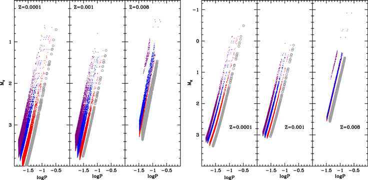
Figure 3. V- (left) and K-band (right) PL relations at varying metallicity for the first four pulsation modes. The color code is the same as in Figure 2.
Download figure:
Standard image High-resolution imageTable 3. Period–Luminosity Relations for the Selected Chemical Abundances, Pulsation Modes, and Filters
| MAG |

|

|

|

|

|

|

|

|
|---|---|---|---|---|---|---|---|---|
| Z = 0.008 | ||||||||
| MU | −0.76 ± 0.10 | −3.064 ± 0.015 | −1.22 ± 0.11 | −3.079 ± 0.018 | −1.61 ± 0.09 | −3.273 ± 0.014 | −1.91 ± 0.07 | −2.930 ± 0.077 |
| MB | −0.68 ± 0.11 | −3.025 ± 0.017 | −1.13 ± 0.12 | −3.031 ± 0.020 | −1.55 ± 0.11 | −3.233 ± 0.016 | −1.78 ± 0.08 | −2.829 ± 0.087 |
| MV | −1.16 ± 0.09 | −3.177 ± 0.014 | −1.61 ± 0.10 | −3.181 ± 0.017 | −1.96 ± 0.09 | −3.348 ± 0.013 | −2.28 ± 0.07 | −3.026 ± 0.072 |
| MR | −1.47 ± 0.08 | −3.291 ± 0.012 | −1.93 ± 0.08 | −3.298 ± 0.014 | −2.22 ± 0.07 | −3.441 ± 0.011 | −2.62 ± 0.06 | −3.176 ± 0.062 |
| MI | −1.81 ± 0.06 | −3.403 ± 0.010 | −2.27 ± 0.07 | −3.415 ± 0.011 | −2.51 ± 0.06 | −3.535 ± 0.009 | −2.97 ± 0.05 | −3.326 ± 0.050 |
| MJ | −2.17 ± 0.05 | −3.541 ± 0.007 | −2.63 ± 0.05 | −3.553 ± 0.009 | −2.81 ± 0.05 | −3.643 ± 0.007 | −3.34 ± 0.04 | −3.494 ± 0.039 |
| MH | −2.49 ± 0.03 | −3.664 ± 0.005 | −2.95 ± 0.04 | −3.677 ± 0.006 | −3.08 ± 0.03 | −3.740 ± 0.005 | −3.67 ± 0.03 | −3.651 ± 0.027 |
| MK | −2.51 ± 0.03 | −3.675 ± 0.005 | −2.97 ± 0.04 | −3.687 ± 0.006 | −3.09 ± 0.03 | −3.748 ± 0.005 | −3.69 ± 0.03 | −3.661 ± 0.027 |
| MF390W | −0.71 ± 0.11 | −3.061 ± 0.017 | −1.18 ± 0.12 | −3.077 ± 0.020 | −1.61 ± 0.11 | −3.293 ± 0.016 | −1.86 ± 0.09 | −2.883 ± 0.088 |
| MF465W | −0.97 ± 0.10 | −3.148 ± 0.016 | −1.44 ± 0.11 | −3.155 ± 0.019 | −1.84 ± 0.10 | −3.352 ± 0.015 | −2.12 ± 0.08 | −2.974 ± 0.082 |
| MF555W | −1.18 ± 0.09 | −3.206 ± 0.015 | −1.64 ± 0.10 | −3.212 ± 0.017 | −2.00 ± 0.09 | −3.389 ± 0.014 | −2.32 ± 0.07 | −3.052 ± 0.075 |
| MF606W | −1.36 ± 0.08 | −3.264 ± 0.013 | −1.83 ± 0.09 | −3.270 ± 0.016 | −2.15 ± 0.08 | −3.431 ± 0.012 | −2.52 ± 0.07 | −3.131 ± 0.068 |
| MF814W | −1.82 ± 0.06 | −3.406 ± 0.010 | −2.28 ± 0.07 | −3.417 ± 0.012 | −2.53 ± 0.06 | −3.539 ± 0.009 | −2.99 ± 0.05 | −3.329 ± 0.051 |
| MF160W | −2.45 ± 0.03 | −3.631 ± 0.005 | −2.91 ± 0.04 | −3.644 ± 0.006 | −3.04 ± 0.03 | −3.707 ± 0.005 | −3.62 ± 0.03 | −3.614 ± 0.029 |
| Z = 0.001 | ||||||||
| MU | −0.39 ± 0.03 | −2.861 ± 0.009 | −0.55 ± 0.07 | −2.731 ± 0.009 | −1.07 ± 0.12 | −2.828 ± 0.014 | −1.70 ± 0.13 | −2.973 ± 0.015 |
| MB | −0.30 ± 0.02 | −2.854 ± 0.005 | −0.60 ± 0.08 | −2.812 ± 0.011 | −1.16 ± 0.14 | −2.908 ± 0.016 | −1.82 ± 0.15 | −3.050 ± 0.017 |
| MV | −0.70 ± 0.02 | −2.952 ± 0.007 | −0.95 ± 0.07 | −2.875 ± 0.009 | −1.47 ± 0.12 | −2.963 ± 0.014 | −2.08 ± 0.13 | −3.089 ± 0.015 |
| MR | −0.99 ± 0.02 | −3.037 ± 0.007 | −1.21 ± 0.06 | −2.941 ± 0.008 | −1.72 ± 0.10 | −3.029 ± 0.012 | −2.29 ± 0.11 | −3.146 ± 0.013 |
| MI | −1.31 ± 0.03 | −3.127 ± 0.008 | −1.50 ± 0.05 | −3.013 ± 0.007 | −1.99 ± 0.09 | −3.100 ± 0.010 | −2.53 ± 0.09 | −3.208 ± 0.010 |
| MJ | −1.67 ± 0.03 | −3.248 ± 0.008 | −1.86 ± 0.04 | −3.126 ± 0.005 | −2.34 ± 0.07 | −3.211 ± 0.008 | −2.83 ± 0.07 | −3.308 ± 0.008 |
| MH | −1.99 ± 0.03 | −3.351 ± 0.009 | −2.14 ± 0.03 | −3.207 ± 0.004 | −2.60 ± 0.05 | −3.290 ± 0.006 | −3.05 ± 0.05 | −3.374 ± 0.006 |
| MK | −2.01 ± 0.03 | −3.363 ± 0.009 | −2.18 ± 0.03 | −3.223 ± 0.004 | −2.63 ± 0.05 | −3.305 ± 0.006 | −3.08 ± 0.05 | −3.388 ± 0.006 |
| MF390W | −0.33 ± 0.03 | −2.877 ± 0.007 | −0.56 ± 0.08 | −2.786 ± 0.010 | −1.11 ± 0.13 | −2.886 ± 0.015 | −1.78 ± 0.14 | −3.039 ± 0.016 |
| MF465W | −0.52 ± 0.03 | −2.930 ± 0.007 | −0.75 ± 0.08 | −2.834 ± 0.010 | −1.29 ± 0.13 | −2.927 ± 0.015 | −1.95 ± 0.14 | −3.070 ± 0.016 |
| MF555W | −0.70 ± 0.03 | −2.970 ± 0.008 | −0.92 ± 0.07 | −2.867 ± 0.010 | −1.45 ± 0.12 | −2.957 ± 0.014 | −2.07 ± 0.13 | −3.091 ± 0.015 |
| MF606W | −0.88 ± 0.03 | −3.016 ± 0.008 | −1.09 ± 0.07 | −2.907 ± 0.009 | −1.60 ± 0.11 | −2.995 ± 0.013 | −2.20 ± 0.12 | −3.123 ± 0.014 |
| MF814W | −1.33 ± 0.03 | −3.134 ± 0.008 | −1.51 ± 0.05 | −3.013 ± 0.007 | −2.01 ± 0.09 | −3.100 ± 0.010 | −2.55 ± 0.09 | −3.210 ± 0.011 |
| MF160W | −1.96 ± 0.03 | −3.330 ± 0.009 | −2.13 ± 0.03 | −3.190 ± 0.004 | −2.58 ± 0.05 | −3.272 ± 0.006 | −3.04 ± 0.06 | −3.356 ± 0.006 |
| Z = 0.0001 | ||||||||
| MU | −0.09 ± 0.04 | −2.700 ± 0.005 | −0.38 ± 0.09 | −2.616 ± 0.008 | −0.72 ± 0.09 | −2.562 ± 0.010 | −1.44 ± 0.13 | −2.812 ± 0.013 |
| MB | −0.13 ± 0.03 | −2.803 ± 0.005 | −0.50 ± 0.10 | −2.743 ± 0.009 | −0.89 ± 0.11 | −2.684 ± 0.012 | −1.64 ± 0.15 | −2.932 ± 0.015 |
| MV | −0.45 ± 0.03 | −2.847 ± 0.005 | −0.77 ± 0.09 | −2.763 ± 0.008 | −1.12 ± 0.10 | −2.705 ± 0.011 | −1.83 ± 0.13 | −2.942 ± 0.013 |
| MR | −0.69 ± 0.03 | −2.901 ± 0.004 | −0.98 ± 0.08 | −2.802 ± 0.007 | −1.32 ± 0.08 | −2.756 ± 0.009 | −2.01 ± 0.11 | −2.989 ± 0.011 |
| MI | −0.98 ± 0.03 | −2.962 ± 0.004 | −1.23 ± 0.07 | −2.847 ± 0.006 | −1.56 ± 0.07 | −2.815 ± 0.008 | −2.23 ± 0.09 | −3.044 ± 0.009 |
| MJ | −1.33 ± 0.03 | −3.066 ± 0.004 | −1.55 ± 0.05 | −2.936 ± 0.005 | −1.89 ± 0.06 | −2.925 ± 0.006 | −2.53 ± 0.07 | −3.149 ± 0.007 |
| MH | −1.61 ± 0.03 | −3.138 ± 0.004 | −1.79 ± 0.05 | −2.990 ± 0.004 | −2.12 ± 0.04 | −2.996 ± 0.005 | −2.73 ± 0.06 | −3.212 ± 0.006 |
| MK | −1.64 ± 0.03 | −3.156 ± 0.004 | −1.82 ± 0.04 | −3.007 ± 0.004 | −2.15 ± 0.04 | −3.012 ± 0.005 | −2.76 ± 0.06 | −3.227 ± 0.006 |
| MF390W | −0.08 ± 0.04 | −2.760 ± 0.005 | −0.42 ± 0.10 | −2.689 ± 0.009 | −0.77 ± 0.11 | −2.621 ± 0.012 | −1.53 ± 0.15 | −2.880 ± 0.015 |
| MF465W | −0.24 ± 0.04 | −2.804 ± 0.005 | −0.57 ± 0.10 | −2.725 ± 0.009 | −0.92 ± 0.11 | −2.648 ± 0.012 | −1.67 ± 0.15 | −2.903 ± 0.015 |
| MF555W | −0.40 ± 0.04 | −2.831 ± 0.005 | −0.71 ± 0.09 | −2.743 ± 0.008 | −1.05 ± 0.10 | −2.672 ± 0.011 | −1.79 ± 0.14 | −2.921 ± 0.014 |
| MF606W | −0.56 ± 0.03 | −2.866 ± 0.005 | −0.86 ± 0.08 | −2.770 ± 0.008 | −1.19 ± 0.09 | −2.709 ± 0.010 | −1.91 ± 0.12 | −2.953 ± 0.012 |
| MF814W | −0.99 ± 0.03 | −2.961 ± 0.004 | −1.24 ± 0.07 | −2.846 ± 0.006 | −1.57 ± 0.07 | −2.812 ± 0.008 | −2.25 ± 0.10 | −3.046 ± 0.010 |
| MF160W | −1.60 ± 0.03 | −3.125 ± 0.004 | −1.78 ± 0.05 | −2.979 ± 0.004 | −2.11 ± 0.04 | −2.983 ± 0.005 | −2.73 ± 0.06 | −3.200 ± 0.006 |
Note. Numerical coefficients of the pulsation equations derived from nonlinear models and expressed as  .
.
Download table as: ASCIITypeset image
The PL relations are very easy to use; however, they do suffer some drawbacks that affect the accuracy in their use as distance indicators, such as the reddening correction to be applied or the intrinsic width of the IS. These problems are partially overtaken when moving to near-infrared wavelengths. However, when we use a reddening-free formulation such as the Wesenheit function, they are very mitigated. In fact, these relations not only are reddening-free by definition but, including a color term, mimic a PL–color relation; thus, they are narrower than the PL relations and can be safely used for accurate distance estimates (see Caputo et al. 2000, for a discussion). Last but not least, it seems that some combinations of the filters of the Wesehneit relations are almost metallicity independent (Fiorentino et al. 2007; Inno et al. 2013; Braga et al. 2015; Marconi et al. 2015). The main con in the use of the Wesenheit relations is that their definition does depend on the adopted reddening law; for the case of RR Lyrae stars, an estimation of this effect on the distance estimate has been discussed in Marconi et al. (2015) and is less than  . We have selected some optical–near-infrared Wesenheit relations that are shown in Table 4. From an inspection of this table, it is clear that the Wesenheit relations do depend on the metallicity term, as happens for the classical Cepheids (Fiorentino et al. 2007). This is different from the recent finding concerning RR Lyrae stars detailed in Marconi et al. (2015). In fact, the authors found a negligible dependence on the metallicity for the filter combination (B, V); however, they also found that the standard deviation decreases when moving to near-infrared bands, thus suggesting that a proper selection of the best relation to be used as a distance indicator has to be based on our knowledge of photometric and spectroscopic uncertainties.
Table 4. Metallicity-dependent Wesehneit Relations for Each Selected Pulsation Mode
| COL | α | β | γ |
|---|---|---|---|
| F Mode | |||
| MV−3.08×(B–V) | −2.51 ± 0.05 | −3.267 ± 0.005 | −0.1697 ± 0.0009 |
| MI−1.43×(V–I) | −2.51 ± 0.05 | −3.385 ± 0.005 | −0.0992 ± 0.0008 |
| MJ−0.39×(V–J) | −2.37 ± 0.04 | −3.380 ± 0.004 | −0.0907 ± 0.0007 |
| MH−0.21×(V–H) | −2.52 ± 0.04 | −3.444 ± 0.004 | −0.0785 ± 0.0007 |
| MK−0.13×(V–K) | −2.47 ± 0.04 | −3.430 ± 0.004 | −0.0822 ± 0.0007 |
| MK−0.27×(V–I) | −2.47 ± 0.04 | −3.423 ± 0.004 | −0.0843 ± 0.0007 |
| FO Mode | |||
| MV−3.08×(B–V) | −2.59 ± 0.08 | −3.136 ± 0.005 | −0.1345 ± 0.0010 |
| MI−1.43×(V–I) | −2.62 ± 0.06 | −3.235 ± 0.004 | −0.0816 ± 0.0007 |
| MJ−0.39×(V–J) | −2.51 ± 0.06 | −3.249 ± 0.004 | −0.0711 ± 0.0007 |
| MH−0.21×(V–H) | −2.65 ± 0.05 | −3.288 ± 0.004 | −0.0654 ± 0.0007 |
| MK−0.13×(V–K) | −2.60 ± 0.06 | −3.284 ± 0.004 | −0.0667 ± 0.0007 |
| MK−0.27×(V–I) | −2.60 ± 0.06 | −3.278 ± 0.004 | −0.0684 ± 0.0007 |
| SO Mode | |||
| MV−3.08×(B–V) | −2.42 ± 0.07 | −3.100 ± 0.004 | −0.0089 ± 0.0010 |
| MI−1.43×(V–I) | −2.46 ± 0.06 | −3.173 ± 0.003 | 0.0177 ± 0.0008 |
| MJ−0.39×(V–J) | −2.35 ± 0.06 | −3.184 ± 0.004 | 0.0347 ± 0.0008 |
| MH−0.21×(V–H) | −2.48 ± 0.05 | −3.211 ± 0.003 | 0.0302 ± 0.0008 |
| MK−0.13×(V–K) | −2.43 ± 0.06 | −3.209 ± 0.003 | 0.0333 ± 0.0008 |
| MK−0.27×(V–I) | −2.42 ± 0.06 | −3.204 ± 0.003 | 0.0317 ± 0.0008 |
| TO Mode | |||
| MV−3.08×(B–V) | −3.14 ± 0.08 | −3.201 ± 0.005 | −0.0822 ± 0.0012 |
| MI−1.43×(V–I) | −3.36 ± 0.05 | −3.368 ± 0.004 | −0.0674 ± 0.0009 |
| MJ−0.39×(V–J) | −3.28 ± 0.06 | −3.387 ± 0.004 | −0.0515 ± 0.0010 |
| MH−0.21×(V–H) | −3.43 ± 0.05 | −3.426 ± 0.003 | −0.0578 ± 0.0008 |
| MK−0.13×(V–K) | −3.37 ± 0.05 | −3.419 ± 0.004 | −0.0541 ± 0.0009 |
| MK−0.27×(V–I) | −3.36 ± 0.05 | −3.412 ± 0.004 | −0.0554 ± 0.0009 |
Note. Numerical coefficients of the pulsation equations derived from nonlinear models and expressed as  =
= 
 .
.
Download table as: ASCIITypeset image
In the case of SXPs, we do not see any trend in the standard deviation ( ) or in the metallicity coefficient (γ) of the Wesenheit relations; we can only claim that the (B, V) filter combination appears to be always the worst to be used for all the pulsation modes, whereas the remaining filter combinations are quite equivalent to each other. In passing, we note that the tree filter combination K, V–I is almost identical to the near-infrared one, K, V–K. This means that, in principle, the use of a triple-band relation as a distance indicator is equivalent to the dual-band one.
We have also computed the color–color relations, shown in Table 5. We highlight that the metallicity term does not seem so important. When not included, it would affect the standard deviation of the relations by ∼0.02 at the maximum. One may notice that the intrinsic scatter of these theoretical relations is very small, with σ(MB−M  mag, as discussed in Caputo et al. (2000). The color–color relations can be very useful to derive an estimation of the reddening E(B–V) of the stellar systems where the SXPs are hosted, in particular by measuring the deviation of the observed colors versus the theoretical predictions.
Table 5. Metallicity-dependent Color–Color Relations for Each Selected Pulsation Mode
| Mode | α | β | γ |
|---|---|---|---|
| F Mode | |||
| MV−MR | 0.097 ± 0.003 | 1.261 ± 0.003 | 0.01302 ± 0.00004 |
| MV−MI | 0.104 ± 0.004 | 0.619 ± 0.002 | 0.01908 ± 0.00005 |
| MV−MJ | 0.127 ± 0.005 | 0.374 ± 0.001 | 0.02144 ± 0.00007 |
| MV−MH | 0.136 ± 0.005 | 0.279 ± 0.001 | 0.02246 ± 0.00007 |
| MV−MK | 0.138 ± 0.005 | 0.271 ± 0.001 | 0.02204 ± 0.00007 |
| FO Mode | |||
| MV−MR | 0.110 ± 0.004 | 1.134 ± 0.002 | 0.01105 ± 0.00004 |
| MV−MI | 0.118 ± 0.005 | 0.541 ± 0.001 | 0.01575 ± 0.00005 |
| MV−MJ | 0.135 ± 0.006 | 0.329 ± 0.001 | 0.01767 ± 0.00006 |
| MV−MH | 0.144 ± 0.006 | 0.244 ± 0.001 | 0.01832 ± 0.00006 |
| MV−MK | 0.145 ± 0.006 | 0.239 ± 0.001 | 0.01808 ± 0.00006 |
| SO Mode | |||
| MV−MR | 0.110 ± 0.004 | 1.093 ± 0.002 | 0.00978 ± 0.00006 |
| MV−MI | 0.116 ± 0.005 | 0.521 ± 0.001 | 0.01398 ± 0.00006 |
| MV−MJ | 0.129 ± 0.006 | 0.324 ± 0.001 | 0.01610 ± 0.00008 |
| MV−MH | 0.136 ± 0.006 | 0.242 ± 0.001 | 0.01656 ± 0.00008 |
| MV−MK | 0.136 ± 0.006 | 0.238 ± 0.001 | 0.01648 ± 0.00008 |
| TO Mode | |||
| MV−MR | 0.088 ± 0.005 | 1.159 ± 0.002 | 0.00588 ± 0.00008 |
| MV−MI | 0.083 ± 0.005 | 0.564 ± 0.001 | 0.00814 ± 0.00009 |
| MV−MJ | 0.090 ± 0.007 | 0.358 ± 0.001 | 0.00969 ± 0.00012 |
| MV−MH | 0.095 ± 0.007 | 0.271 ± 0.001 | 0.00986 ± 0.00012 |
| MV−MK | 0.095 ± 0.007 | 0.268 ± 0.001 | 0.00987 ± 0.00012 |
Note. Numerical coefficients of the pulsation equations derived from nonlinear models and expressed as B–V =  COL
COL  .
.
Download table as: ASCIITypeset image
Finally, we provide in Table 6 the mass- and metallicity-dependent PL relations for all the selected bands. These relations can give us fundamental constraints on the stellar mass of the BSSs, as extensively described in the Introduction, and they are the main goal of this paper. These equations can be used any time we have a detection in at least one photometric band of an SXP, once the pulsation mode and a chemical composition are assumed. The latter case is quite obvious for most of the GCs in our Galaxy, for which accurate spectroscopic abundances are available nowadays in literature (e.g., Carretta et al. 2009).
Table 6. Mass–Period–Luminosity–Metallicity Relations for Each Selected Pulsation Mode
| MAG | α | β | γ | δ |
|---|---|---|---|---|
| F Mode | ||||
| MU | 0.19 ± 0.02 | −0.224 ± 0.004 | −0.62 ± 0.01 | 0.0628 ± 0.0005 |
| MB | 0.22 ± 0.03 | −0.154 ± 0.004 | −0.42 ± 0.01 | 0.0641 ± 0.0007 |
| MV | 0.07 ± 0.02 | −0.228 ± 0.004 | −0.66 ± 0.01 | 0.0523 ± 0.0007 |
| MR | −0.09 ± 0.02 | −0.295 ± 0.004 | −0.88 ± 0.01 | 0.0439 ± 0.0007 |
| MI | −0.31 ± 0.02 | −0.375 ± 0.004 | −1.16 ± 0.01 | 0.0380 ± 0.0006 |
| MJ | −0.63 ± 0.02 | −0.477 ± 0.004 | −1.54 ± 0.01 | 0.0341 ± 0.0005 |
| MH | −0.95 ± 0.01 | −0.563 ± 0.004 | −1.87 ± 0.01 | 0.0337 ± 0.0004 |
| MK | −0.99 ± 0.01 | −0.573 ± 0.004 | −1.91 ± 0.01 | 0.0330 ± 0.0004 |
| MF390W | 0.21 ± 0.02 | −0.183 ± 0.004 | −0.50 ± 0.01 | 0.0628 ± 0.0006 |
| MF475W | 0.14 ± 0.02 | −0.202 ± 0.004 | −0.57 ± 0.01 | 0.0555 ± 0.0007 |
| MF555W | 0.06 ± 0.02 | −0.232 ± 0.004 | −0.67 ± 0.01 | 0.0509 ± 0.0007 |
| MF606W | −0.02 ± 0.02 | −0.266 ± 0.004 | −0.78 ± 0.01 | 0.0471 ± 0.0007 |
| MF814W | −0.31 ± 0.02 | −0.371 ± 0.004 | −1.14 ± 0.01 | 0.0387 ± 0.0006 |
| MF160W | −0.94 ± 0.01 | −0.563 ± 0.004 | −1.86 ± 0.01 | 0.0335 ± 0.0004 |
| FO Mode | ||||
| MU | 0.04 ± 0.02 | −0.238 ± 0.002 | −0.68 ± 0.00 | 0.0606 ± 0.0003 |
| MB | 0.06 ± 0.03 | −0.182 ± 0.002 | −0.54 ± 0.01 | 0.0610 ± 0.0003 |
| MV | −0.07 ± 0.02 | −0.225 ± 0.002 | −0.68 ± 0.01 | 0.0545 ± 0.0003 |
| MR | −0.20 ± 0.02 | −0.269 ± 0.002 | −0.83 ± 0.01 | 0.0499 ± 0.0003 |
| MI | −0.38 ± 0.02 | −0.329 ± 0.002 | −1.02 ± 0.01 | 0.0463 ± 0.0003 |
| MJ | −0.66 ± 0.02 | −0.413 ± 0.002 | −1.32 ± 0.01 | 0.0432 ± 0.0002 |
| MH | −0.98 ± 0.01 | −0.508 ± 0.001 | −1.65 ± 0.00 | 0.0393 ± 0.0002 |
| MK | −1.01 ± 0.01 | −0.514 ± 0.002 | −1.68 ± 0.00 | 0.0391 ± 0.0002 |
| MF390W | 0.06 ± 0.02 | −0.201 ± 0.002 | −0.59 ± 0.00 | 0.0607 ± 0.0003 |
| MF475W | 0.00 ± 0.02 | −0.203 ± 0.002 | −0.61 ± 0.00 | 0.0565 ± 0.0003 |
| MF555W | −0.06 ± 0.02 | −0.223 ± 0.002 | −0.67 ± 0.00 | 0.0540 ± 0.0003 |
| MF606W | −0.13 ± 0.02 | −0.246 ± 0.002 | −0.75 ± 0.01 | 0.0519 ± 0.0003 |
| MF814W | −0.37 ± 0.02 | −0.324 ± 0.002 | −1.01 ± 0.01 | 0.0470 ± 0.0003 |
| MF160W | −0.94 ± 0.01 | −0.496 ± 0.002 | −1.61 ± 0.01 | 0.0410 ± 0.0002 |
| SO Mode | ||||
| MU | 0.19 ± 0.03 | −0.153 ± 0.002 | −0.38 ± 0.01 | 0.0709 ± 0.0005 |
| MB | 0.21 ± 0.03 | −0.120 ± 0.002 | −0.29 ± 0.01 | 0.0693 ± 0.0005 |
| MV | 0.13 ± 0.03 | −0.148 ± 0.002 | −0.38 ± 0.01 | 0.0682 ± 0.0005 |
| MR | 0.06 ± 0.03 | −0.171 ± 0.002 | −0.46 ± 0.01 | 0.0675 ± 0.0005 |
| MI | −0.02 ± 0.03 | −0.192 ± 0.003 | −0.53 ± 0.01 | 0.0672 ± 0.0005 |
| MJ | −0.07 ± 0.03 | −0.190 ± 0.003 | −0.54 ± 0.01 | 0.0664 ± 0.0005 |
| MH | −0.05 ± 0.03 | −0.164 ± 0.004 | −0.46 ± 0.01 | 0.0641 ± 0.0005 |
| MK | −0.04 ± 0.03 | −0.157 ± 0.004 | −0.44 ± 0.01 | 0.0639 ± 0.0005 |
| MF390W | 0.20 ± 0.03 | −0.134 ± 0.002 | −0.33 ± 0.01 | 0.0703 ± 0.0005 |
| MF475W | 0.16 ± 0.03 | −0.140 ± 0.002 | −0.36 ± 0.01 | 0.0690 ± 0.0004 |
| MF555W | 0.13 ± 0.03 | −0.152 ± 0.002 | −0.40 ± 0.01 | 0.0685 ± 0.0004 |
| MF606W | 0.09 ± 0.03 | −0.164 ± 0.002 | −0.44 ± 0.01 | 0.0682 ± 0.0004 |
| MF814W | −0.02 ± 0.03 | −0.193 ± 0.003 | −0.54 ± 0.01 | 0.0678 ± 0.0005 |
| MF160W | −0.06 ± 0.03 | −0.171 ± 0.004 | −0.48 ± 0.01 | 0.0650 ± 0.0005 |
| TO Mode | ||||
| MU | −0.07 ± 0.02 | −0.129 ± 0.001 | −0.41 ± 0.00 | 0.0453 ± 0.0004 |
| MB | −0.02 ± 0.03 | −0.093 ± 0.001 | −0.31 ± 0.00 | 0.0463 ± 0.0004 |
| MV | −0.11 ± 0.02 | −0.121 ± 0.001 | −0.40 ± 0.00 | 0.0439 ± 0.0004 |
| MR | −0.21 ± 0.02 | −0.151 ± 0.002 | −0.50 ± 0.01 | 0.0415 ± 0.0004 |
| MI | −0.37 ± 0.02 | −0.197 ± 0.002 | −0.66 ± 0.01 | 0.0384 ± 0.0004 |
| MJ | −0.63 ± 0.02 | −0.263 ± 0.002 | −0.89 ± 0.01 | 0.0344 ± 0.0003 |
| MH | −1.05 ± 0.02 | −0.375 ± 0.002 | −1.29 ± 0.01 | 0.0263 ± 0.0003 |
| MK | −1.06 ± 0.02 | −0.376 ± 0.002 | −1.30 ± 0.01 | 0.0263 ± 0.0003 |
| MF390W | −0.04 ± 0.02 | −0.107 ± 0.001 | −0.35 ± 0.00 | 0.0462 ± 0.0004 |
| MF475W | −0.06 ± 0.02 | −0.109 ± 0.001 | −0.36 ± 0.00 | 0.0451 ± 0.0004 |
| MF555W | −0.10 ± 0.02 | −0.121 ± 0.001 | −0.40 ± 0.00 | 0.0441 ± 0.0004 |
| MF606W | −0.16 ± 0.02 | −0.136 ± 0.001 | −0.45 ± 0.00 | 0.0430 ± 0.0004 |
| MF814W | −0.35 ± 0.02 | −0.191 ± 0.002 | −0.64 ± 0.01 | 0.0394 ± 0.0004 |
| MF160W | −0.98 ± 0.02 | −0.356 ± 0.002 | −1.22 ± 0.01 | 0.0289 ± 0.0003 |
Note. Numerical coefficients of the pulsation equations derived from nonlinear models and expressed as logM/ =
=  MAG
MAG 
 .
.
5. THEORY VERSUS OBSERVATIONS: THE CASE OF ω CEN
In this section we discuss the interesting case of ω Cen, with the final aim of deriving its SXP mass distribution. This is the most massive and the brightest GC-like stellar system in our Galaxy, and it is characterized by a quite complex star formation history. In fact at odds with the vast majority of GCs in the Galaxy, it harbors multiple populations with different iron abundance spanning a huge range of metallicity (almost 2 dex: ![$-2.4\;\lesssim \;[{Fe}/H]\;\lesssim \;-0.4$](https://content.cld.iop.org/journals/0004-637X/810/1/15/revision1/apj518003ieqn64.gif) ).6
The properties of these subpopulations have been deeply investigated over the past 20 years using both photometry (Lee & Carney 1999; Pancino et al. 2000; Ferraro et al. 2004; Sollima et al. 2005; Calamida et al. 2009; Bellini et al. 2010) and spectroscopy (Origlia et al. 2003; Johnson & Pilachowski 2010; Pancino et al. 2011a, 2011b; Moni Bidin et al. 2012; Simpson & Cottrell 2013; Villanova et al. 2014). Such peculiar characteristics locate ω Cen in between the properties of GCs and the more luminous dwarf galaxies (Tolstoy et al. 2009). Moreover, it harbors the largest population of BSSs detected so far in a stellar system (even considering only the brightest portion of the sequence, Ferraro et al. [2006a] identified more than 300 BSSs) and possibly the largest population of SXPs.
).6
The properties of these subpopulations have been deeply investigated over the past 20 years using both photometry (Lee & Carney 1999; Pancino et al. 2000; Ferraro et al. 2004; Sollima et al. 2005; Calamida et al. 2009; Bellini et al. 2010) and spectroscopy (Origlia et al. 2003; Johnson & Pilachowski 2010; Pancino et al. 2011a, 2011b; Moni Bidin et al. 2012; Simpson & Cottrell 2013; Villanova et al. 2014). Such peculiar characteristics locate ω Cen in between the properties of GCs and the more luminous dwarf galaxies (Tolstoy et al. 2009). Moreover, it harbors the largest population of BSSs detected so far in a stellar system (even considering only the brightest portion of the sequence, Ferraro et al. [2006a] identified more than 300 BSSs) and possibly the largest population of SXPs.
In particular, there are a few photometric surveys specifically dedicated to detecting and characterizing its variables: the two most complete ones have been carried out using CCD photometry on the 1.0 m Swope telescope at Las Campanas Observatory by the Ogle Gravitational Lensing Experiment (OGLE; Kaluzny et al. 1996) and by the Cluster Ages Experiment (CASE; Kaluzny et al. 2004; Olech et al. 2005). OGLE has monitored ω Cen in V and I filters, whereas CASE in B and V filters. On the basis of their periods and their location in the CMD, the OGLE project detected and classified 24 of its variables as SXPs, whereas the CASE project increased this sample to 68 SXPs. A recent compilation of these data has been presented in Cohen & Sarajedini (2012), where B and V magnitudes are taken from the recent work presented in Kaluzny et al. (2004) and V–I color is taken from Kaluzny et al. (1996). However, the sparse sampling obtained in I band of the OGLE time-series photometry does not allow us to derive a robust V–I color (see Kaluzny et al. 1996, for a detailed discussion); thus, we decided to use only stars included in the CASE sample for which both B and V photometric bands are available; we collected a subsample of 54 stars.
To properly compare theory and observations, we need to adopt (a) distance modulus and reddening, (b) metal content, and (c) pulsation modes.
5.1. Distance Modulus
First, we assume a distance modulus and a reddening for ω Cen, i.e.,  14.09 and E(B−V) = 0.13 mag (Kaluzny et al. 2002). This is an accurate estimation of the distance obtained using detached eclipsing double-line spectroscopic binaries, and it turns out to be broadly consistent with recent results obtained using the RR Lyrae (
 14.18 ± 0.04 mag) and Type II Cepheid (
 14.07 ± 0.07 mag) stars photometered in Ks band from the VISTA survey (Navarrete et al. 2014, 2015), which are also very similar to those of Del Principe et al. (2006) and Matsunaga et al. (2006) based on the same distance indicators.
5.2. Metallicity Selection
Since no direct measures of the metallicity of SXPs in Omega Centauri are available in the literature, we derived some constraints from the metallicity distribution of the BSS population. To do this, we measured the metal content in 39 BSSs, extracted from a larger sample including 109 BSSs and studied by Mucciarelli et al. (2014). The spectra were acquired by using the high-resolution spectrograph FLAMES-GIRAFFE (Pasquini et al. 2002) at ESO-VLT, under three different programs, 077.D–0696(Å), 081.D–0356(Å), and 089.D–0298(Å), with several gratings: HR5A (R ∼ 18500,  4340–4587 Å), HR14A (R ∼ 18000,
  6308–6701 Å), HR15N (R ∼ 17000,
  6470–6790 Å), HR2 (R ∼ 19600,
  3854–4049 Å), and HR4 (R ∼ 20350,
  4340–4587 Å). The atmospheric parameters (effective temperature, gravity, and microturbulence) and rotational velocities for the stars are discussed in Mucciarelli et al. (2014). Owing to the high rotation of many BSSs in the original sample, a reliable measure of metallicity has been obtained only for 39 BSSs by using 5–10 iron lines. The metallicity distribution of these stars spans from
  to −0.5 with
 ![$\langle [\mathrm{Fe}/{\rm{H}}]\;\rangle =-1.07$](https://content.cld.iop.org/journals/0004-637X/810/1/15/revision1/apj518003ieqn74.gif) ± 0.09 (
± 0.09 ( 0.6). However, the effective temperatures for most of the BSSs are higher than 8000 K and thus allow the occurrence of a diffusion process called radiative levitation (see Lovisi et al. 2012, 2013 for details). This process affects the surface chemical composition, mimicking a higher metal content. If we consider only the 10 coldest (
 K) BSSs that are not greatly affected by levitation, the iron content spans from
  to
to  with
with ![$\langle [\mathrm{Fe}/{\rm{H}}]\rangle \;=\;-1.41$](https://content.cld.iop.org/journals/0004-637X/810/1/15/revision1/apj518003ieqn79.gif) ± 0.11 (
± 0.11 ( 0.3). These values suggest that also SXPs may reflect the same metallicity spread of the subgiant stellar populations.
In order to account for such a complex metallicity distribution, we have decided to use the theoretical scenarios7
with [Fe/H] = −1.65 (Z ∼ 0.001) and with [Fe/H] = −0.7 (Z ∼ 0.008). These values describe both the abundant metal-poor peak and the metal-rich tail of the ω Cen metallicity distribution (Johnson & Pilachowski 2010), thus bracketing the behavior of most of the populations in this cluster, as shown in Figure 4. In this figure a direct comparison between the SXPs and the ISs for the two selected metallicities is shown. Theory and observations agree quite well, with a few exceptions of very red stars (B −  mag, five triangles) that we have excluded from the following analysis. In this figure we have overplotted two alpha-enhanced evolutionary tracks (for each metal assumption) for masses that fully define the magnitude–color location of the observed SXPs.
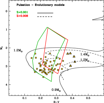
Figure 4. Distribution in the CMDs of 54 SXPs (squares) in ω Cen for which we have both B and V bands from the CASE project. We also show the IS regions for Z = 0.001 (green) and 0.008 (red). The very red (B–V  mag) SXPs excluded from the mass analysis are highlighted with triangles. We have also shown the alpha-enhanced evolutionary tracks for Z = 0.001 (M = 0.9 and 1.2
  ; solid lines) and for Z = 0.008 (M = 1.2 and 1.4
  ; dashed lines) from the BASTI website (Pietrinferni et al. 2004).
Download figure:
Standard image High-resolution image5.3. Pulsation Mode Identification
Pulsation modes are fixed using the theoretical predictions in the V-band PL planes; thus, they depend on the metallicity adopted (see Figure 5). The pulsation mode is in fact assigned to look at the minimum distance of each star to the four theoretical V-band PLs. In Figure 5 we have also shown the B-band PL relations to check the consistency of the pulsation mode set in V band. For the metallicity Z = 0.001 (left panels) we can assign the following modes: 13 F, 22 FO, 9 SO, and 5 TO. This is the first time that we are able to properly identify such high-overtone modes; in fact, they were broadly classified as higher than F variables from McNamara (2011). Furthermore, this author derived an observational PL relation for F mode stars that turns out to be much flatter ( ) than the predicted ones (
 ; see Table 3). This is essentially due to the different mode classification; in fact, most of our F and FO are considered as F mode SXPs by McNamara (2011). However, we remember here that the distance modulus estimated applying such an observed PL relation is in very good agreement with that used in our analysis. For
  (Figure 5, right panels) we considered only those stars that fall in the region covered by models; as a consequence, we have excluded many stars showing luminosities lower than predicted by pulsation and evolutionary models. In this case, we can assign a pulsation mode only for 25 stars; these are divided into 15 F, 6 FO, and 4 SO.

Figure 5. B- (top) and V-band (bottom) theoretical PL relations compared with SXPs for Z = 0.001 (left) and 0.008 (right). Synthetic models are shown to give an idea of the PL dispersion. The pulsation modes are color coded as in Figures 2 and 3. Magenta, cyan, orange, and green indicate our classification of SXPs as third-overtone, second-overtone, first-overtone, and fundamental modes, respectively.
Download figure:
Standard image High-resolution image
Finally, we can use the pulsation modes for each selected metallicity to estimate masses using B and V mass-dependent PL relations.8
The values are given in Table 7, and their mean values are  with
with 
 and
and  with
with 
 for Z = 0.001 and Z = 0.008, respectively, fully in agreement with the evolutionary scenario shown in Figure 4 (left panel).
Table 7. Pulsation Masses
| Z = 0.001 | Z = 0.008 |
|---|---|
Mass ( ) from B Band ) from B Band |
|
 = 1.14 ± 0.01 = 1.14 ± 0.01 |
 = 1.37 ± 0.02 = 1.37 ± 0.02 |
 = 1.05 ± 0.01 = 1.05 ± 0.01 |
 = 1.28 ± 0.02 = 1.28 ± 0.02 |
 = 1.13 ± 0.02 = 1.13 ± 0.02 |
 = 1.31 ± 0.02 = 1.31 ± 0.02 |
 = 1.13 ± 0.02 = 1.13 ± 0.02 |
|
Mass ( ) from V Band ) from V Band |
|
 =1.14 ± 0.01 =1.14 ± 0.01 |
 = 1.36 ± 0.03 = 1.36 ± 0.03 |
 = 1.05 ± 0.01 = 1.05 ± 0.01 |
 = 1.30 ± 0.02 = 1.30 ± 0.02 |
 = 1.16 ± 0.02 = 1.16 ± 0.02 |
 = 1.34 ± 0.02 = 1.34 ± 0.02 |
 = 1.15 ± 0.02 = 1.15 ± 0.02 |
⋯ |
Download table as: ASCIITypeset image
6. SUMMARY AND FINAL REMARKS
We developed a new and homogenous theoretical framework to account for pulsation properties of SXPs identified in different stellar systems, namely, Galactic GCs and nearby dwarf galaxies. We constructed different sequences of pulsation models that cover a broad range in stellar masses, luminosities, and chemical compositions (Z = 0.0001, Y = 0.24; Z = 0.001, Y = 0.245; Z = 0.008, Y = 0.25).
The pulsation scenario we developed relies on several physical assumptions:
- a.The current pulsation models account for radial oscillations. However, SXPs located on the MS often display nonradial oscillation together with the radial ones.
- b.The intrinsic parameters (stellar masses and luminosities) adopted to construct the pulsation models are based on evolutionary tracks of single stars, while SXPs and the other nonpulsating BSSs probably originated from the evolution of binary systems.
- c.The pulsation relations were derived assuming a constant star formation rate in the computation of synthetic stellar populations (IACstar code). This means that we are assuming single-mass evolutionary tracks to describe the behavior of BSSs. The last two assumptions imply that we are assuming intrinsic parameters (stellar masses, luminosities, chemical compositions) that are more homogeneous than observed. The actual properties are strongly correlated with the evolutionary status and the time elapsed from the formation of cluster SXPs.
The above assumptions become even more severe in dealing with SXPs in ω Cen, since this is one of the few GCs showing a well-defined spread in iron abundance. However, we found that predicted and empirical properties for SXPs (49) in ω Cen agree quite well. The theoretical ISs for Z = 0.001 and 0.008 transformed into the observational plane (V, B–V CMD) take account of the entire sample. A few (five) red SXPs are located outside the predicted instability. It is not clear whether this discrepancy might be due to a slightly more metal-rich chemical composition or to limits in the adopted color–temperature transformations or in the pulsation models close to the red edge of the IS. Note that this is the region of the IS in which convective transport becomes more efficient and quenches radial oscillations.
We provide new PL relations for optical and NIR bands. We found that the slopes of the quoted relations become steeper when moving from optical to NIR bands, suggesting that the latter are better diagnostics to estimate individual distances of SXPs. In this context it is worth mentioning that metal-rich SXPs, in contrast with classical Cepheids (Fiorentino et al. 2013), are brighter than metal-poor ones and their slopes are steeper, increasing the metal content.
The use of nonlinear radial models allowed us to investigate the topology of high overtones. We found that the occurrence of third overtones is strongly correlated with the metal content. They approach a stable nonlinear limit cycle in the metal-poor regime but almost disappear for the most metal-rich chemical composition (Z = 0.008).
We used predicted PL relations in the B and V bands to perform a detailed mode identification for a significant fraction of SXPs in ω Cen. On the basis of the mode identification and of mass-dependent PLZ relations we provided an estimate of their pulsation masses. We found that the mean mass of SXPs does depend on the adopted chemical abundance. The mass distributions range from  (
( 0.06)
0.06)  for Z = 0.001 using 49 objects to
  = 1.33 (
 0.03)
0.03)  for Z = 0.008 using 25 objects. The current pulsation masses are well above the MSTO of canonical stellar populations in ω Cen, i.e., 0.8
  (Castellani et al. 2007).
The current stellar mass distribution of SXPs in ω Cen agrees quite well with similar estimates based on their pulsation period (see discussion in McNamara 2011). In a forthcoming investigation we plan to investigate in more detail the predicted pulsation properties (luminosity and velocity amplitudes) of SXPs and to compare them with SXPs in GCs and in nearby dwarf galaxies available in the literature.
Moreover and even more importantly, we plan to investigate the dependence of the topology of the IS and of the pulsation properties on the helium content (Lombardi et al. 1996; Sills et al. 2009). Detailed hydrodynamical simulations of BSS formation indicate that they might have helium abundances higher than canonical cluster stars.
The increase in the helium content in canonical radial pulsators causes a steady increase in the pulsation period but small changes in the pulsation observables (amplitudes, modal stability). However, SXPs have surface gravities that are almost 2 dex larger than classical radial variables. The coupling between driving mechanisms, efficiency of convective transport across the partial ionization regions, and chemical compositions need to be investigated on a more quantitative basis. The preliminary comparison between theory and observations appears promising, a good viaticum for the forthcoming investigations.
This research is part of the project Cosmic-Lab (http://www.cosmic-lab.eu) funded by the European Research Council under contract ERC-2010-AdG-267675. G.F. has been supported also by the FIRB 2013 (grant RBFR13J716).
Footnotes
- 6
- 7
We have verified that no significant effects on our results are caused by a metallicity change from Z = 0.0006 to Z = 0.001.
- 8
We note here that the use of mass-dependent PLC relations is not recommended and will not be further discussed. This happens because the color term turns out to have a very high coefficient that changes significantly with the pulsation mode. For this reason a minimal change in the color produces a large effect on the computed stellar mass. In particular, the estimated final mass shows an unreasonable trend with pulsation mode, i.e., increasing the pulsation mode means larger masses.