


ABSTRACT
As hundreds of gas giant planets have been discovered, we study how these planets form and evolve in different stellar environments, specifically in multiple stellar systems. In such systems, stellar companions may have a profound influence on gas giant planet formation and evolution via several dynamical effects such as truncation and perturbation. We select 84 Kepler Objects of Interest (KOIs) with gas giant planet candidates. We obtain high-angular resolution images using telescopes with adaptive optics (AO) systems. Together with the AO data, we use archival radial velocity data and dynamical analysis to constrain the presence of stellar companions. We detect 59 stellar companions around 40 KOIs for which we develop methods of testing their physical association. These methods are based on color information and galactic stellar population statistics. We find evidence of suppressive planet formation within 20 AU by comparing stellar multiplicity. The stellar multiplicity rate (MR) for planet host stars is  % within 20 AU. In comparison, the stellar MR is 18% ± 2% for the control sample, i.e., field stars in the solar neighborhood. The stellar MR for planet host stars is 34% ± 8% for separations between 20 and 200 AU, which is higher than the control sample at 12% ± 2%. Beyond 200 AU, stellar MRs are comparable between planet host stars and the control sample. We discuss the implications of the results on gas giant planet formation and evolution.
Export citation and abstract BibTeX RIS
1. INTRODUCTION
Almost half of Sun-like stars are members of binary or multiple star systems (hereafter MSS, Duquennoy & Mayor 1991; Raghavan et al. 2010). During the formation of a star–planet system, the presence of a companion star is likely to perturb or truncate the protoplanetary disk (e.g., Holman & Wiegert 1999; Jang-Condell 2007). These effects would affect the formation rate of planets around the stellar components of MSS. Indeed, observations of star-forming regions show that protoplanetary disks around MSS have shorter lifetimes than disks around single star systems (hereafter SSS, Kraus et al. 2012). Furthermore, after planet formation, dynamical interactions with stellar companions could affect the orbital evolution of a planet and its survival rate via perturbation (Wu & Murray 2003; Naoz et al. 2012), disk-driven migration (Lin & Papaloizou 1986; Tanaka et al. 2002), and planet–planet scattering (Rasio & Ford 1996; Chatterjee et al. 2008).
Despite many theoretical and numerical studies of planets in MSS, the planet occurrence rate in MSS is still uncertain. There have been numerous estimates of the planet occurrence rate for solar-type stars based on the Kepler results (e.g., Howard et al. 2012; Fressin et al. 2013); however, these studies do not distinguish between planet host stars in SSS or MSS. The lack of stellar multiplicity information prevents us from comparing the planet occurrence rate between SSS and MSS. The comparison would provide insights into the influence of stellar companions on planet formation. The discovery of thousands of planet candidates from the Kepler mission (Borucki et al. 2011; Batalha et al. 2013; Burke et al. 2014) provides a unique opportunity to study planets in MSS (e.g., Wang et al. 2014a)
There are two ways of studying planets in MSS. First, one can select a sample of known MSS and then search for planets around each of the component stars (the Planet-Quest approach, e.g., Konacki 2005; Eggenberger et al. 2007; Konacki et al. 2009; Toyota et al. 2009). Unfortunately, for ground based surveys, the detection efficiency of planets in MSS is affected by flux contamination from the additional stellar components (Wright et al. 2012). Flux contamination also reduces the signal-to-noise ratio (S/N) of a transiting planet (Fressin et al. 2013; Wang et al. 2014a). On the other hand, the Star-Quest approach is an effective way to study planets in MSS. Using a sample of known stars with planets, it is possible to determine the fraction of MSS in that sample (e.g., Luhman & Jayawardhana 2002; Patience et al. 2002; Wang et al. 2014b; Ngo et al. 2015). From a technical standpoint, it is much easier to detect stellar companions than planetary companions, making the Star-Quest approach much easier and more sensitive to lower mass planets. Previous observational studies have suggested that the presence of a stellar companion suppresses planet formation (e.g., Eggenberger et al. 2011). However, these studies have not fully considered biases in target selection and planet detection or the observational incompleteness in the search for stellar companions of planet host stars. Wang et al. (2014a) discuss the above concerns and find that planet formation is suppressed by stellar companions with separations up to 1500 AU.
Wang et al. (2014a, 2014b) summarize the works following the Star-Quest approach prior to 2014. Since then, more progress has been made. These new results suggest that visual stellar companions are not rare around planet host stars. Using the Lucky Imaging technique, Lillo-Box et al. (2014) find that 32.8% of Kepler planet host stars have at least one visual stellar companion within 6''. Based on adaptive optics (AO) imaging of 87 Kepler planet host stars, Dressing et al. (2014) find that 31.0% of planet host stars have stellar companions within 4''. Law et al. (2014) observe 715 Kepler stars with planet candidates with the Robo-AO system. They find 7.4% of Kepler planet host stars have stellar companions within 2 5. However, the fraction of gravitationally bound companions is uncertain from these surveys. Using the speckle imaging technique, Horch et al. (2014) detect 49 stellar companions within 1 arcsec around over 600 Kepler stars with planet candidates. The majority of the detected companions are likely to be gravitationally bound to the planet host stars based on a statistical argument. Accounting for detection incompleteness, they conclude that the stellar multiplicity rate (MR) for planet host stars is similar to stars in the solar neighborhood. Gilliland et al. (2015) observe 23 Kepler stars with small and cool planet candidates using the Hubble Space Telescope. They find evidence that physically associated stellar companions are more common around planet host stars than around field stars in the solar neighborhood. The Kepler stars in the aforementioned studies have an average Kepler magnitude of 13.5. Assuming that they are solar-type stars, the average distance is ∼600–700 pc. More recently, Ngo et al. (2015) focus on a sample of host stars for hot Jupiters (HJs) that were discovered and confirmed by ground-based observations. They use AO imaging and conduct multiple-epoch observations to confirm physical association by measuring common proper motions of stellar components. The stellar MR for HJ host stars is almost twice as high as that for stars in the solar neighborhood for stellar separations between 50 and 2000 AU. The overabundance of stellar companions for HJ host stars suggests the positive role of stellar companions in HJ formation and evolution.
While rapid progress has been made since 2014, there are still a number of issues for the Star-Quest approach. First, there is a selection bias against MSS for work on planets detected by ground-based observations. MSS with small separations and considerable flux contamination are usually excluded in ground-based surveys for planets (e.g., Wright et al. 2012). The selection bias is difficult to quantify and correct, so converting the measured stellar MR to planet occurrence rate is challenging (Wang et al. 2014a). Second, most studies focus on a single detection technique for stellar companions. The high-angular resolution imaging technique has been the dominant method. However, the physical association of stellar companions is difficult to assess for Kepler stars. This becomes an issue when calculating the stellar MR which concerns only gravitationally bound companions. Third, the imaging techniques are not effective in detecting stellar companions within or near the diffraction limits of telescopes, which correspond to 20–50 AU in physical separation. Stellar companions at smaller separations can be more effectively detected by measuring the radial velocity (RV). So far, only a few studies following the Star-Quest approach use the RV technique in combination with the high-angular resolution imaging technique, which dramatically increases the search completeness for stellar companions (Knutson et al. 2014; Wang et al. 2014a; Ngo et al. 2015).
Finally, the control sample to be compared is not a perfect sample. Field stars in the solar neighborhood usually serve as a control sample for stars without planets, but studies on planet occurrence rate suggest that the majority of stars host at least one planet (e.g., Mayor et al. 2011; Howard et al. 2012; Dressing & Charbonneau 2013; Fressin et al. 2013). In order to construct a more meaningful control sample, we can find other stars that do not have planets down to a certain mass and up to a certain orbital separation (e.g., Eggenberger et al. 2007), or we can continue to use the field stars as a control sample but set a planet mass/radius and separation range to limit the level of contamination of planet host stars. For example, if we consider only gas giant planets within ∼1 AU, then the stars in the solar neighborhood can serve as a reasonable control sample because fewer than 10% of stars have gas giant planets within 1 AU (Cumming et al. 2008; Mayor et al. 2011).
To address the above issues, we have conducted a search for stellar companions for 84 Kepler stars with gas giant planets within ∼1 AU. This sample of stars is not biased against MSS because the Kepler mission does not apply a selection criterion that excludes MSS (Brown et al. 2011). The typical FWHM of images for Kepler target selection is 25 and thus these images are ineffective at distinguishing binary stars. We use both RV data and high-angular resolution imaging data for these stars, so the search completeness is high compared to surveys employing only one technique. We assess the physical association of detected stellar companions using (1) their color information and (2) a statistical argument based on a galactic stellar population model. We can compare the stellar MR for this sample to that for field stars in the solar neighborhood without a significant contamination of planet host stars in the control sample. After these issues are resolved, we can study the influence of stellar companions on gas giant planet formation with the sample 84 Kepler planet host stars.
The paper is organized as follows. We describe the sample of Kepler stars with gas giant planets in Section 2. AO observation and data reduction for these stars are presented in Section 3. We also discuss the physical association of detected stellar companions in Section 4. We synthesize the results of different techniques in the search for stellar companions in Section 5. These techniques include the RV and AO imaging techniques and the dynamical analysis. The stellar MR of Kepler stars with gas giant planets is given in Section 6. The discussion and the summary are given in Sections 7 and 8.
2. SAMPLE DESCRIPTION
From the NASA Exoplanet Archive,4
we select Kepler Objects of Interest (KOIs) that satisfy the following criteria: (1) disposition of either Candidate or Confirmed, (2) stellar effective temperature ( ) lower than 6500 K, (3) stellar surface gravity (
 ) higher than 4.0, (4) Kepler magnitude (KP) brighter than 14th mag, (5) with at least one gas giant planet (
 ). In total, we select 84 KOIs with 97 gas giant planets. Stellar and orbital parameters for these KOIs are given in Table 1. The median distance of these KOIs is 580 pc. There are 27 multi-planet systems among 84 KOIs.
Table 1. RV and AO Data for 97 KOIs
| KOI | RV | AO | ||||||||||||||
|---|---|---|---|---|---|---|---|---|---|---|---|---|---|---|---|---|
| KOI | KIC | α | δ | KP |

|

|
d | #PL | R
|
Period |

|

|
#RV | Telescope | Band | This Work |
| (deg) | (deg) | (mag) | (K) | (cgs) | (pc) | (R ) ) |
(day) | (MJD) | (MJD) | |||||||
| K00001.01 | 11446443 | 286.808472 | 49.316399 | 11.338 | 5814.00 | 4.380 | 207.0 | 1 | 14.40 ± 1.60 | 2.470613 | 54216.610352 | 56208.227539 | 18 | Keck | JHK | ✓ |
| K00003.01 | 10748390 | 297.709351 | 48.080853 | 9.174 | 4766.00 | 4.590 | 38.8 | 1 | 4.68 ± 0.18 | 4.887800 | 54336.352539 | 56485.626953 | 42 | WIYN | rz | ⋯ |
| K00005.01 | 8554498 | 289.739716 | 44.647419 | 11.665 | 5861.00 | 4.190 | 286.6 | 2 | 5.66 ± 0.72 | 4.780329 | 54983.515625 | 56486.439453 | 21 | KeckPalomar | JK | ⋯ |
| K00010.01 | 6922244 | 281.288116 | 42.451080 | 13.563 | 6025.00 | 4.110 | 919.7 | 1 | 15.90 ± 2.10 | 3.522499 | 54983.540039 | 55781.534180 | 50 | Palomar | J | ⋯ |
| K00017.01 | 10874614 | 296.837250 | 48.239944 | 13.303 | 5826.00 | 4.420 | 494.3 | 1 | 11.07 ± 0.54 | 3.234700 | 54984.560547 | 55043.519531 | 10 | Palomar | J | ⋯ |
| K00020.01 | 11804465 | 286.243439 | 50.040379 | 13.438 | 6011.00 | 4.230 | 608.4 | 1 | 17.60 ± 2.50 | 4.437963 | 55014.412109 | 55761.325195 | 16 | Palomar | J | ⋯ |
| K00022.01 | 9631995 | 282.629669 | 46.323360 | 13.435 | 5972.00 | 4.410 | 593.4 | 1 | 11.27 ± 0.70 | 7.891450 | 55014.403320 | 55792.438477 | 16 | Palomar | J | ⋯ |
| K00046.01 | 10905239 | 283.255493 | 48.355232 | 13.770 | 5764.00 | 4.400 | 604.1 | 2 | 4.33 ± 0.37 | 3.487688 | ⋯ | ⋯ | ⋯ | Keck | K | ✓ |
| K00063.01 | 11554435 | 289.226166 | 49.548199 | 11.582 | 5721.00 | 4.470 | 212.3 | 1 | 6.31 ± 0.31 | 9.434158 | ⋯ | ⋯ | ⋯ | Keck | K | ✓ |
| K00094.02 | 6462863 | 297.333069 | 41.891121 | 12.205 | 6184.00 | 4.181 | 463.6 | 4 | 4.22 ± 0.42 | 10.423707 | ⋯ | ⋯ | ⋯ | MMT | JK | ⋯ |
| K00094.03 | 6462863 | 297.333069 | 41.891121 | 12.205 | 6184.00 | 4.181 | 463.6 | 4 | 6.73 ± 0.67 | 54.319930 | ⋯ | ⋯ | ⋯ | MMT | JK | ⋯ |
| K00094.01 | 6462863 | 297.333069 | 41.891121 | 12.205 | 6184.00 | 4.181 | 463.6 | 4 | 11.40 ± 1.10 | 22.343001 | ⋯ | ⋯ | ⋯ | MMT | JK | ⋯ |
| K00097.01 | 5780885 | 288.581512 | 41.089809 | 12.885 | 5934.00 | 4.040 | 789.7 | 1 | 16.10 ± 2.00 | 4.885489 | 55106.878906 | 55115.871094 | 9 | MMT | JK | ⋯ |
| K00098.01 | 10264660 | 287.708832 | 47.333050 | 12.128 | 6395.00 | 4.150 | 446.2 | 1 | 10.00 ± 1.40 | 6.790123 | 55440.500987 | 56533.433594 | 7 | MMTPalomar | JK | |
| K00108.02 | 4914423 | 288.984558 | 40.064529 | 12.287 | 5975.00 | 4.330 | 354.6 | 2 | 4.46 ± 0.52 | 179.601000 | 55073.468750 | 56145.498047 | 22 | KeckPalomar | JK | ⋯ |
| K00119.01 | 9471974 | 294.559174 | 46.062328 | 12.654 | 5632.00 | 4.440 | 313.0 | 2 | 3.90 ± 2.60 | 49.184310 | ⋯ | ⋯ | ⋯ | Palomar | JK | ✓ |
| K00127.01 | 8359498 | 289.607971 | 44.345421 | 13.938 | 5731.00 | 4.450 | 617.4 | 1 | 10.93 ± 0.47 | 3.578783 | ⋯ | ⋯ | ⋯ | Palomar | J | ⋯ |
| K00128.01 | 11359879 | 296.200592 | 49.140121 | 13.758 | 5786.00 | 4.420 | 579.8 | 1 | 11.97 ± 0.85 | 4.942783 | 55284.481445 | 55509.075195 | 30 | Keck | K | ✓ |
| K00131.01 | 7778437 | 299.097534 | 43.497589 | 13.797 | 6411.00 | 4.400 | 937.3 | 1 | 9.00 ± 3.20 | 5.014233 | ⋯ | ⋯ | ⋯ | Keck | K | ✓ |
| K00135.01 | 9818381 | 285.240845 | 46.668251 | 13.958 | 6082.00 | 4.370 | 810.1 | 1 | 10.56 ± 0.46 | 3.024095 | 55752.008789 | 55806.833984 | 8 | Keck | K | ✓ |
| K00137.01 | 8644288 | 298.079437 | 44.746319 | 13.549 | 5385.00 | 4.430 | 421.9 | 3 | 4.75 ± 0.43 | 7.641571 | 55075.508789 | 56146.484375 | 20 | Palomar | J | ⋯ |
| K00137.02 | 8644288 | 298.079437 | 44.746319 | 13.549 | 5385.00 | 4.430 | 421.9 | 3 | 6.01 ± 0.54 | 14.858940 | 55075.508789 | 56146.484375 | 20 | Palomar | J | ⋯ |
| K00139.01 | 8559644 | 291.653168 | 44.688271 | 13.492 | 5952.00 | 4.380 | 612.0 | 2 | 7.34 ± 0.66 | 224.797120 | ⋯ | ⋯ | ⋯ | Lick | J | ⋯ |
| K00141.01 | 12105051 | 288.038300 | 50.651611 | 13.687 | 5425.00 | 4.500 | 463.1 | 1 | 5.43 ± 0.29 | 2.624234 | ⋯ | ⋯ | ⋯ | MMT | JK | ⋯ |
| K00152.01 | 8394721 | 300.517120 | 44.381580 | 13.914 | 6405.00 | 4.420 | 897.1 | 4 | 6.10 ± 1.90 | 52.091100 | ⋯ | ⋯ | ⋯ | Palomar | K | ✓ |
| K00157.03 | 6541920 | 297.115112 | 41.909142 | 13.709 | 5685.00 | 4.380 | 514.8 | 6 | 4.18 ± 0.76 | 31.995467 | 55440.500987 | 56533.433594 | 7 | Palomar | K | ✓ |
| K00179.02 | 9663113 | 297.045410 | 46.328701 | 13.955 | 6081.00 | 4.420 | 771.2 | 2 | 5.00 ± 1.70 | 572.397900 | ⋯ | ⋯ | ⋯ | Keck | K | ✓ |
| K00244.01 | 4349452 | 286.638397 | 39.487881 | 10.734 | 6103.00 | 4.070 | 313.5 | 2 | 6.51 ± 0.89 | 12.720365 | 55366.602539 | 56519.408203 | 104 | KeckPalomar | JK | ⋯ |
| K00279.01 | 12314973 | 295.486511 | 51.013500 | 11.684 | 6418.00 | 4.280 | 268.6 | 3 | 5.10 ± 1.60 | 28.454899 | ⋯ | ⋯ | ⋯ | Keck | K | ⋯ |
| K00289.02 | 10386922 | 282.945648 | 47.574905 | 12.747 | 5812.00 | 4.458 | 348.4 | 2 | 5.04 ± 0.00 | 296.637100 | 56449.400391 | 56532.291016 | 5 | KeckPalomar | K | ✓ |
| K00318.01 | 8156120 | 288.153992 | 44.068821 | 12.211 | 6285.00 | 4.290 | 415.8 | 1 | 5.19 ± 0.49 | 38.583360 | ⋯ | ⋯ | ⋯ | Palomar | K | ✓ |
| K00319.01 | 8684730 | 290.117523 | 44.872940 | 12.711 | 5952.00 | 4.190 | 421.3 | 1 | 7.50 ± 1.10 | 46.151590 | ⋯ | ⋯ | ⋯ | Palomar | K | ✓ |
| K00340.01 | 10616571 | 297.664673 | 47.801392 | 13.057 | 5811.00 | 4.400 | 417.3 | 1 | 16.80 ± 1.40 | 23.673188 | ⋯ | ⋯ | ⋯ | Palomar | K | ✓ |
| K00344.01 | 11015108 | 283.340271 | 48.549042 | 13.400 | 5984.00 | 4.340 | 597.5 | 1 | 3.80 ± 1.60 | 39.309240 | ⋯ | ⋯ | ⋯ | Palomar | K | ✓ |
| K00351.02 | 11442793 | 284.433502 | 49.305161 | 13.804 | 6330.00 | 4.430 | 870.7 | 6 | 6.80 ± 3.00 | 210.596590 | ⋯ | ⋯ | ⋯ | WIYN | rz | ⋯ |
| K00351.01 | 11442793 | 284.433502 | 49.305161 | 13.804 | 6330.00 | 4.430 | 870.7 | 6 | 9.80 ± 4.20 | 331.643000 | ⋯ | ⋯ | ⋯ | WIYN | rz | ⋯ |
| K00366.01 | 3545478 | 291.664185 | 38.619255 | 11.714 | 6207.00 | 4.180 | 352.1 | 1 | 10.60 ± 4.60 | 75.112019 | ⋯ | ⋯ | ⋯ | KeckPalomar | K | ✓ |
| K00367.01 | 4815520 | 284.472168 | 39.911812 | 11.105 | 5569.00 | 4.360 | 153.6 | 1 | 4.98 ± 0.71 | 31.578680 | ⋯ | ⋯ | ⋯ | KeckPalomar | JK | ✓ |
| K00372.01 | 6471021 | 299.122437 | 41.866760 | 12.391 | 5872.00 | 4.487 | 355.2 | 1 | 8.52 ± 0.23 | 125.630640 | ⋯ | ⋯ | ⋯ | MMT | K | ⋯ |
| K00375.01 | 12356617 | 291.201202 | 51.144279 | 13.293 | 5757.00 | 4.140 | 778.2 | 1 | 10.40 ± 1.40 | 988.881118 | ⋯ | ⋯ | ⋯ | Palomar | K | ✓ |
| K00377.02 | 3323887 | 285.573975 | 38.400902 | 13.803 | 5777.00 | 4.450 | 619.4 | 3 | 8.22 ± 0.59 | 38.907202 | 55342.448242 | 56506.363281 | 16 | Palomar | JK | ⋯ |
| K00377.01 | 3323887 | 285.573975 | 38.400902 | 13.803 | 5777.00 | 4.450 | 619.4 | 3 | 8.28 ± 0.59 | 19.273938 | 55342.448242 | 56506.363281 | 16 | Palomar | JK | ⋯ |
| K00633.01 | 4841374 | 293.427032 | 39.942429 | 13.871 | 6070.00 | 4.030 | 640.1 | 1 | 5.80 ± 1.80 | 161.479000 | ⋯ | ⋯ | ⋯ | Palomar | K | ✓ |
| K00638.01 | 5113822 | 295.559418 | 40.236271 | 13.595 | 5980.00 | 4.310 | 575.9 | 2 | 3.80 ± 1.20 | 23.636883 | ⋯ | ⋯ | ⋯ | MMT | K | ⋯ |
| K00638.02 | 5113822 | 295.559418 | 40.236271 | 13.595 | 5980.00 | 4.310 | 575.9 | 2 | 3.90 ± 1.30 | 67.093500 | ⋯ | ⋯ | ⋯ | MMT | K | ⋯ |
| K00672.02 | 7115785 | 291.169525 | 42.640808 | 13.998 | 5524.00 | 4.410 | 524.6 | 3 | 4.03 ± 0.41 | 41.749990 | ⋯ | ⋯ | ⋯ | Keck | K | ✓ |
| K00680.01 | 7529266 | 292.287323 | 43.197281 | 13.643 | 6327.00 | 4.350 | 786.9 | 1 | 8.00 ± 2.40 | 8.600145 | ⋯ | ⋯ | ⋯ | Keck | K | ✓ |
| K00682.01 | 7619236 | 295.197998 | 43.269508 | 13.916 | 5592.00 | 4.250 | 632.7 | 1 | 10.80 ± 1.40 | 562.142400 | ⋯ | ⋯ | ⋯ | Keck | K | ✓ |
| K00683.01 | 7630229 | 297.824310 | 43.258381 | 13.714 | 5887.00 | 4.390 | 647.6 | 1 | 6.00 ± 0.77 | 278.122200 | ⋯ | ⋯ | ⋯ | Palomar | K | ✓ |
| K00686.01 | 7906882 | 296.840759 | 43.647121 | 13.579 | 5559.00 | 4.470 | 494.5 | 1 | 11.40 ± 4.40 | 52.513565 | ⋯ | ⋯ | ⋯ | Palomar | K | ✓ |
| K00697.01 | 8878187 | 289.000885 | 45.154270 | 13.684 | 5779.00 | 4.050 | 1315.7 | 1 | 4.24 ± 0.75 | 3.032154 | ⋯ | ⋯ | ⋯ | Keck | JHK | ✓ |
| K00707.03 | 9458613 | 289.077545 | 46.005219 | 13.988 | 5904.00 | 4.030 | 1236.7 | 5 | 4.10 ± 0.36 | 31.784660 | ⋯ | ⋯ | ⋯ | Keck | K | ✓ |
| K00707.02 | 9458613 | 289.077545 | 46.005219 | 13.988 | 5904.00 | 4.030 | 1236.7 | 5 | 4.69 ± 0.41 | 41.027950 | ⋯ | ⋯ | ⋯ | Keck | K | ✓ |
| K00707.01 | 9458613 | 289.077545 | 46.005219 | 13.988 | 5904.00 | 4.030 | 1236.7 | 5 | 5.50 ± 0.48 | 21.775754 | ⋯ | ⋯ | ⋯ | Keck | K | ✓ |
| K00716.01 | 9846348 | 297.492157 | 46.694519 | 13.754 | 6115.00 | 4.490 | 713.2 | 1 | 6.80 ± 3.20 | 26.893084 | ⋯ | ⋯ | ⋯ | Palomar | K | ✓ |
| K01162.01 | 10528068 | 288.868225 | 47.759430 | 12.783 | 6138.00 | 4.280 | 490.7 | 1 | 4.40 ± 2.30 | 158.692400 | ⋯ | ⋯ | ⋯ | Palomar | K | ✓ |
| K01206.01 | 3756801 | 293.954590 | 38.899971 | 13.642 | 5754.00 | 4.110 | 826.9 | 1 | 6.20 ± 1.90 | 422.917678 | ⋯ | ⋯ | ⋯ | Keck | K | ✓ |
| K01274.01 | 8800954 | 283.256805 | 45.087780 | 13.354 | 5310.00 | 4.550 | 356.9 | 1 | 4.73 ± 0.28 | 704.962626 | ⋯ | ⋯ | ⋯ | Palomar | K | ✓ |
| K01311.01 | 10713616 | 283.532959 | 48.094261 | 13.498 | 6188.00 | 4.200 | 648.2 | 1 | 4.20 ± 1.70 | 83.577520 | ⋯ | ⋯ | ⋯ | Palomar | K | ✓ |
| K01335.01 | 4155328 | 291.020142 | 39.220680 | 13.968 | 6222.00 | 4.040 | 1385.0 | 1 | 8.60 ± 2.70 | 127.832900 | ⋯ | ⋯ | ⋯ | Palomar | K | ✓ |
| K01353.02 | 7303287 | 297.465332 | 42.882839 | 13.956 | 6260.00 | 4.080 | 1094.5 | 2 | 3.80 ± 1.10 | 34.543630 | ⋯ | ⋯ | ⋯ | Palomar | K | ✓ |
| K01353.01 | 7303287 | 297.465332 | 42.882839 | 13.956 | 6260.00 | 4.080 | 1094.5 | 2 | 18.60 ± 5.30 | 125.865460 | ⋯ | ⋯ | ⋯ | Palomar | K | ✓ |
| K01375.01 | 6766634 | 288.320435 | 42.261414 | 13.709 | 6169.00 | 4.358 | 594.0 | 1 | 6.78 ± 0.00 | 321.213900 | ⋯ | ⋯ | ⋯ | KeckPalomar | JHK | ✓ |
| K01411.01 | 9425139 | 298.995087 | 45.909512 | 13.377 | 5753.00 | 4.410 | 502.0 | 1 | 7.05 ± 0.84 | 305.056500 | ⋯ | ⋯ | ⋯ | Palomar | K | ✓ |
| K01431.01 | 11075279 | 287.022278 | 48.681938 | 13.460 | 5649.00 | 4.460 | 486.8 | 1 | 8.45 ± 0.48 | 345.161300 | 56472.390625 | 56532.501953 | 6 | Palomar | K | ✓ |
| K01439.01 | 11027624 | 290.851776 | 48.521339 | 12.849 | 5930.00 | 4.090 | 719.2 | 1 | 7.80 ± 1.10 | 394.610700 | 55075.273438 | 56531.312500 | 6 | Palomar | K | ✓ |
| K01474.01 | 12365184 | 295.417877 | 51.184761 | 13.005 | 6293.00 | 4.270 | 552.0 | 1 | 9.30 ± 1.20 | 69.732970 | ⋯ | ⋯ | ⋯ | Palomar | K | ✓ |
| K01478.01 | 12403119 | 288.848633 | 51.209049 | 12.450 | 5493.00 | 4.417 | 288.4 | 1 | 5.26 ± 0.35 | 76.133540 | ⋯ | ⋯ | ⋯ | Palomar | K | ✓ |
| K01645.01 | 11045383 | 298.210938 | 48.559158 | 13.418 | 5197.00 | 4.530 | 379.9 | 1 | 10.31 ± 3.10 | 41.166759 | ⋯ | ⋯ | ⋯ | Palomar | K | ✓ |
| K01658.01 | 4570949 | 294.192108 | 39.618999 | 13.308 | 6422.00 | 4.320 | 750.6 | 1 | 12.35 ± 0.67 | 1.544930 | ⋯ | ⋯ | ⋯ | Keck | K | ✓ |
| K01684.01 | 6048024 | 293.534485 | 41.329899 | 12.849 | 6387.00 | 4.430 | 616.1 | 1 | 7.30 ± 2.60 | 62.815570 | ⋯ | ⋯ | ⋯ | Palomar | K | ✓ |
| K01779.02 | 9909735 | 298.482819 | 46.793621 | 13.297 | 5812.00 | 4.140 | 586.3 | 2 | 5.00 ± 1.70 | 11.815018 | ⋯ | ⋯ | ⋯ | KeckPalomar | K | ✓ |
| K01779.01 | 9909735 | 298.482819 | 46.793621 | 13.297 | 5812.00 | 4.140 | 586.3 | 2 | 5.80 ± 1.90 | 4.662723 | ⋯ | ⋯ | ⋯ | KeckPalomar | K | ✓ |
| K01783.02 | 10005758 | 289.341431 | 46.988239 | 13.929 | 6235.00 | 4.460 | 845.5 | 2 | 5.20 ± 1.90 | 284.042300 | ⋯ | ⋯ | ⋯ | Palomar | K | ✓ |
| K01783.01 | 10005758 | 289.341431 | 46.988239 | 13.929 | 6235.00 | 4.460 | 845.5 | 2 | 8.50 ± 3.10 | 134.479720 | ⋯ | ⋯ | ⋯ | Palomar | K | ✓ |
| K01784.01 | 10158418 | 297.646057 | 47.167488 | 13.592 | 5853.00 | 4.540 | 574.0 | 1 | 5.20 ± 3.00 | 5.007410 | ⋯ | ⋯ | ⋯ | Keck | JHK | ✓ |
| K01792.01 | 8552719 | 288.971649 | 44.624531 | 12.160 | 5689.00 | 4.440 | 300.1 | 3 | 4.61 ± 0.27 | 88.407030 | ⋯ | ⋯ | ⋯ | Keck | K | ⋯ |
| K01800.01 | 11017901 | 285.268585 | 48.560009 | 12.394 | 5600.00 | 4.430 | 307.9 | 1 | 6.20 ± 2.10 | 7.794300 | ⋯ | ⋯ | ⋯ | Keck | K | ✓ |
| K01805.02 | 4644952 | 288.811951 | 39.770660 | 13.828 | 5708.00 | 4.080 | 789.5 | 3 | 4.30 ± 1.20 | 31.782260 | ⋯ | ⋯ | ⋯ | Keck | K | ✓ |
| K01805.01 | 4644952 | 288.811951 | 39.770660 | 13.828 | 5708.00 | 4.080 | 789.5 | 3 | 5.60 ± 1.50 | 6.941344 | ⋯ | ⋯ | ⋯ | Keck | K | ✓ |
| K01808.01 | 7761918 | 294.743317 | 43.461208 | 12.487 | 6278.00 | 4.350 | 424.4 | 1 | 4.00 ± 1.60 | 89.192840 | ⋯ | ⋯ | ⋯ | Palomar | K | ✓ |
| K01812.01 | 6279974 | 290.126526 | 41.601082 | 13.742 | 6285.00 | 4.420 | 778.7 | 1 | 4.80 ± 1.80 | 0.805263 | ⋯ | ⋯ | ⋯ | Keck | K | ✓ |
| K01825.01 | 5375194 | 295.300079 | 40.556591 | 13.895 | 5545.00 | 4.060 | 904.3 | 1 | 4.20 ± 1.10 | 13.522604 | ⋯ | ⋯ | ⋯ | Palomar | K | ✓ |
| K02672.01 | 11253827 | 296.132812 | 48.977402 | 11.921 | 5565.00 | 4.330 | 236.0 | 2 | 5.30 ± 2.10 | 88.516580 | ⋯ | ⋯ | ⋯ | Palomar | K | ⋯ |
| K02674.01 | 8022489 | 289.651245 | 43.824421 | 13.349 | 5973.00 | 4.260 | 501.1 | 3 | 7.30 ± 2.60 | 197.510340 | ⋯ | ⋯ | ⋯ | Palomar | K | ✓ |
| K02677.01 | 9958387 | 294.757690 | 46.831120 | 13.460 | 6409.00 | 4.340 | 694.7 | 1 | 6.50 ± 1.00 | 237.788200 | ⋯ | ⋯ | ⋯ | Palomar | K | ✓ |
| K03444.02 | 5384713 | 297.429199 | 40.561909 | 13.693 | 3842.00 | 4.664 | 122.4 | 4 | 5.74 ± 3.20 | 60.326632 | ⋯ | ⋯ | ⋯ | KeckPalomar | JK | ✓ |
| K03663.01 | 12735740 | 289.763611 | 51.962601 | 12.620 | 6007.00 | 4.340 | 394.8 | 1 | 11.29 ± 0.03 | 282.525503 | ⋯ | ⋯ | ⋯ | ⋯ | ⋯ | ⋯ |
| K03678.01 | 4150804 | 289.791595 | 39.285328 | 12.888 | 5650.00 | 4.313 | 413.8 | 1 | 9.12 ± 0.04 | 160.885644 | ⋯ | ⋯ | ⋯ | Palomar | K | ✓ |
| K03787.01 | 7813039 | 288.439117 | 43.505249 | 13.891 | 5993.00 | 4.355 | 741.5 | 1 | 9.17 ± 1.10 | 141.733971 | ⋯ | ⋯ | ⋯ | Palomar | K | ✓ |
| K03791.02 | 5437945 | 288.474854 | 40.651360 | 13.771 | 6340.00 | 4.163 | 932.2 | 2 | 5.65 ± 0.21 | 220.130023 | ⋯ | ⋯ | ⋯ | Keck | JK | ⋯ |
| K03791.01 | 5437945 | 288.474854 | 40.651360 | 13.771 | 6340.00 | 4.163 | 932.2 | 2 | 7.21 ± 0.11 | 440.785197 | ⋯ | ⋯ | ⋯ | Keck | JK | ⋯ |
| K03811.01 | 4638237 | 286.153107 | 39.714901 | 13.906 | 5551.00 | 4.518 | 505.5 | 1 | 6.98 ± 0.99 | 290.140253 | ⋯ | ⋯ | ⋯ | Palomar | K | ✓ |
| K03823.01 | 4820550 | 286.771454 | 39.983822 | 13.922 | 5817.00 | 4.544 | 663.9 | 1 | 5.54 ± 0.08 | 202.117797 | ⋯ | ⋯ | ⋯ | Palomar | K | ✓ |
| K03875.01 | 11911561 | 290.149139 | 50.239178 | 13.579 | 6022.00 | 4.027 | 660.4 | 1 | 4.73 ± 0.70 | 8.870420 | ⋯ | ⋯ | ⋯ | Keck | K | ✓ |
| K03907.01 | 7137213 | 296.997803 | 42.653320 | 12.642 | 6498.00 | 4.081 | 610.0 | 1 | 4.05 ± 0.88 | 28.643425 | ⋯ | ⋯ | ⋯ | KeckPalomar | JHK | ✓ |
| K05515.01 | 8429817 | 291.452271 | 44.431751 | 13.952 | 6247.00 | 4.255 | 806.9 | 1 | 8.88 ± 1.50 | 6.263490 | ⋯ | ⋯ | ⋯ | Keck | JHK | ✓ |
There are 19 KOIs with RV observations. We obtain RV data from the Kepler Community Follow-up Observation Program5 (CFOP). The majority of the RV data (14 out of 19 ) were taken with the HIRES instrument (Vogt et al. 1994) and reported in Marcy et al. (2014). Exceptions are KOI-1 (TrES-2, O'Donovan et al. 2006), KOI-3 (HAT-P-11 b, Bakos et al. 2010), KOI-97 (Kepler-7 b, Latham et al. 2010), KOI-128 (Kepler-15 b, Endl et al. 2011), and KOI-135 (Kepler-43 b, Bonomo et al. 2012). The Modified Julian Dates (MJDs) of the first and last RV data points and the number of RV data points for each KOI are given in Table 1.
For KOIs with high-angular resolution images from CFOP, we use the images to search for stellar companions. These images were taken at different telescopes including Keck, Palomar, MMT, Lick, and WIYN. For KOIs whose high-angular resolution images are not available, we have taken AO images using the PHARO (Palomar High Angular Resolution Observer) instrument (Brandl et al. 1997; Hayward et al. 2001) at the Palomar 200 inch telescope and the NIRC2 instrument (Wizinowich et al. 2000) at the Keck II telescope. In total, we have taken AO images for 60 out of the 84 KOIs. Telescope and photometric band information is given in Table 1. The KOIs with AO images taken through this work are also indicated in Table 1.
3. AO OBSERVATION AND DATA REDUCTION
3.1. AO Imaging with PHARO at Palomar
We observed 40 KOIs in the sample with the PHARO instrument (Brandl et al. 1997; Hayward et al. 2001) at the Palomar 200 inch telescope. The observations were made between UT July 13 and 17 in 2014 with seeing varying between 10 and 25. PHARO is behind the Palomar-3000 AO system, which provides an on-sky Strehl of 86% in the K band (Burruss et al. 2014). The pixel scale of PHARO is 25 mas pixel−1. With a mosaic 1K × 1K detector, the field of view (FOV) is  25''. We normally obtained the first image in K band with a 5 point dither pattern, which had a throw of 25. The exposure time was set such that the peak flux of the KOI is at least 10,000 ADU for each frame, which is within the linear range of the detector. If a stellar companion was detected, we observed the KOI in the J and H bands.
3.2. AO Imaging with NIRC2 at Keck II
We observed 27 KOIs in the sample with the NIRC2 instrument (Wizinowich et al. 2000) at the Keck II telescope. The observations were made on UT July 18 and August 18 in 2014 with excellent/good seeing between 03 to 08. NIRC2 is a near-infrared imager designed for the Keck AO system. We selected the narrow camera mode, which has a pixel scale of 10 mas pixel−1. The FOV is thus  10'' for a mosaic 1K × 1K detector. We started the observation in the K band for each KOI. The exposure time setting is the same as the PHARO observation: we ensured that the peak flux is at least 10,000 ADU for each frame. We used a 3 point dither pattern with a throw of 25. We avoided the lower left quadrant in the dither pattern because it has a much higher instrumental noise than the other three quadrants on the detector. We continued observations of a KOI in the J and H bands if any stellar companions were found.
3.3. Contrast Curve and Detections
The raw data were processed using standard techniques to replace bad pixels, flat-field, subtract thermal background, align, and co-add frames. We calculated the 5σ detection limit as follows. We defined a series of concentric annuli centering on the star. For the concentric annuli, we calculated the median and the standard deviation of flux for pixels within these annuli. We used the value of five times the standard deviation above the median as the 5σ detection limit. The median contrast curve and the 1σ deviation of K band AO images we used in this paper are shown in Figure 1. Also plotted are detected stellar companions as indicated by asterisks in Figure 1. These companions are brighter than the contrast curve, so the significance of detections is at least 5σ. In total, 59 stellar companions were detected around 40 KOIs. Their stellar and orbital properties are summarized in Table 2.
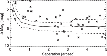
Figure 1. Median 5σ contrast curve for AO images of 84 KOIs shown with the solid line. Dashed lines are 1σ deviation of the contrast curve. Detections within 5'' are shown as asterisks. When analyzing the detection completeness, each KOI is treated individually for the observation band in which the AO image was taken. A total of 59 visual companions around 40 KOIs are detected (Table 2).
Download figure:
Standard image High-resolution imageTable 2. Visual Companion Detections with AO Data
| KOI | Δ Mag | Separation | Distance | Detection | P.A. | Association | Ref. | ||
|---|---|---|---|---|---|---|---|---|---|
| Primary | Secondary | Significance | Probability | ||||||
| (mag) | (arcsec) | (AU) | (pc) | (pc) | (σ) | (deg) | |||
| K00001 | 4.0 (i) | 1.13 | ⋯ | ⋯ |

|
⋯ | 135.0 | ⋯ | L14 |
| 4.3 (r) | 1.11 | ⋯ | ⋯ | ⋯ | ⋯ | 135.5 | 0.98 | H14 | |
| 3.3 (z) | 1.11 | ⋯ | ⋯ | ⋯ | ⋯ | 136.3 | 0.99 | H14 | |
| 2.8 (J) | 1.12 | 232.6 |

|
⋯ | 233.5 | 136.2 | 1.00 | this work | |
| 2.5 (H) | 1.11 | 230.5 |

|
⋯ | 383.6 | 136.3 | 1.00 | this work | |
| 2.4 (K) | 1.12 | 230.9 |

|
⋯ | 68.5 | 136.5 | 1.00 | this work | |
| K00005 | 2.3 (K) | 0.14 | 40.3 |

|
⋯ | 19.2 | 308.9 | 1.00 | CFOP |
K00010
|
7.7 (J) | 3.04 | 2795.9 |

|
⋯ | ⋯ | 94.3 | 0.00 | A12 |
| K00010 | 6.2 (J) | 3.74 | 3439.7 |

|
⋯ | 14.9 | 89.3 | 0.15 | A12 |
| K00017 | 3.8 (J) | 4.01 | 1982.1 |

|
⋯ | 132.6 | 39.9 | 0.75 | A12 |
K00020
|
7.9 (J) | 5.04 | 3066.3 |

|
⋯ | ⋯ | 139.6 | 0.00 | A12 |
| K00097 | 4.0 (J) | 1.90 | 1500.4 |

|

|
49.8 | 105.1 | 0.90 | A12 |
| 4.0 (K) | 1.91 | 1508.3 |

|
⋯ | 81.0 | 105.1 | 0.89 | A12 | |
| K00098 | 0.1 (i) | 0.29 | ⋯ | ⋯ |

|
⋯ | 140.0 | ⋯ | L14 |
| 0.5 (r) | 0.29 | ⋯ | ⋯ | ⋯ | ⋯ | 140.0 | 1.00 | H14 | |
| 0.7 (z) | 0.29 | ⋯ | ⋯ | ⋯ | ⋯ | 140.3 | 1.00 | H14 | |
| 0.3 (J) | 0.27 | 120.5 |

|
⋯ | ⋯ | 143.7 | 1.00 | A12 | |
| 0.4 (K) | 0.28 | 124.9 |

|
⋯ | 15.7 | 143.5 | 1.00 | A12 | |
| K00098 | 6.2 (J) | 5.60 | 2498.7 |

|

|
20.8 | 306.3 | 0.13 | A12 |
| 5.6 (K) | 5.59 | 2494.3 |

|
⋯ | 12.0 | 306.1 | 0.16 | A12 | |
| K00098 | 7.2 (J) | 6.20 | 2766.1 |

|

|
9.5 | 237.9 | 0.00 | this work |
| 6.3 (K) | 6.21 | 2769.5 |

|
⋯ | 5.1 | 237.9 | 0.24 | this work | |
K00108
|
7.2 (J) | 2.44 | 865.2 |

|
⋯ | ⋯ | 74.9 | 0.35 | A12 |
K00108
|
7.2 (J) | 4.87 | 1726.9 |

|
⋯ | ⋯ | 112.4 | 0.00 | A12 |
| K00119 | 0.9 (i) | 1.05 | ⋯ | ⋯ |

|
⋯ | 118.0 | ⋯ | L14 |
| 0.2 (J) | 1.05 | 327.5 |

|
⋯ | 116.2 | 118.4 | 0.60 | this work | |
| 0.2 (K) | 1.05 | 327.5 |

|
⋯ | 96.7 | 118.4 | 1.00 | this work | |
| K00137 | 4.1 (J) | 5.59 | 2359.2 |

|
⋯ | 116.7 | 349.8 | 0.57 | A12 |
K00137
|
7.9 (J) | 4.80 | 2025.1 |

|
⋯ | ⋯ | 340.5 | 0.00 | A12 |
K00137
|
7.5 (J) | 4.98 | 2101.1 |

|
⋯ | ⋯ | 136.3 | 0.00 | A12 |
| K00141 | 1.4 (i) | 1.10 | ⋯ | ⋯ |

|
⋯ | 11.0 | ⋯ | L14 |
| 1.2 (J) | 1.06 | 490.9 |

|
⋯ | 192.1 | 13.9 | 0.99 | A12 | |
| 1.4 (K) | 1.06 | 490.9 |

|
⋯ | 242.4 | 13.5 | 0.99 | A12 | |
| K00152 | 5.7 (K) | 2.49 | 2230.1 |

|
⋯ | 6.0 | 29.5 | 0.23 | this work |
| K00157 | 4.4 (K) | 1.36 | 698.7 |

|
⋯ | 6.0 | 179.9 | 0.94 | this work |
| K00157 | 4.7 (K) | 4.09 | 2104.3 |

|
⋯ | 7.7 | 238.0 | 0.35 | this work |
| K00279 | 3.5 (r) | 0.92 | ⋯ | ⋯ |

|
⋯ | 246.6 | 0.99 | H14 |
| 3.1 (z) | 0.92 | ⋯ | ⋯ | ⋯ | ⋯ | 247.2 | 0.99 | H14 | |
| 2.3 (K) | 0.93 | 250.4 |

|
⋯ | 111.8 | 246.9 | 1.00 | CFOP | |
| K00340 | 5.4 (K) | 5.34 | 2227.7 |

|
⋯ | 6.0 | 57.6 | 0.10 | this work |
| K00344 | 3.5 (K) | 4.13 | 2470.2 |

|
⋯ | 45.9 | 178.9 | 0.68 | this work |
| K00344 | 5.2 (K) | 3.55 | 2123.6 |

|
⋯ | 9.7 | 210.6 | 0.34 | this work |
| K00366 | 6.5 (K) | 7.00 | 2464.4 |

|
⋯ | 5.6 | 70.1 | 0.02 | this work |
K00372
|
8.6 (K) | 2.49 | 884.4 |

|
⋯ | ⋯ | 157.8 | 0.00 | A12 |
K00372
|
8.0 (K) | 3.56 | 1264.5 |

|
⋯ | ⋯ | 56.9 | 0.00 | A12 |
K00372
|
8.2 (K) | 4.99 | 1772.4 |

|
⋯ | ⋯ | 170.7 | 0.00 | A12 |
K00372
|
4.0 (K) | 5.94 | 2109.9 |

|
⋯ | ⋯ | 32.7 | 0.64 | A12 |
| K00375 | 3.3 (K) | 5.47 | 4254.0 |

|
⋯ | 25.4 | 157.0 | 0.64 | this work |
| K00375 | 4.6 (K) | 3.19 | 2486.2 |

|
⋯ | 5.9 | 305.5 | 0.56 | this work |
| K00377 | 4.5 (J) | 5.90 | 3654.5 |

|

|
37.5 | 91.7 | 0.31 | A12 |
| 4.2 (K) | 5.89 | 3648.3 |

|
⋯ | 101.0 | 91.7 | 0.34 | A12 | |
K00377
|
6.8 (J) | 2.79 | 1728.1 |

|

|
⋯ | 37.9 | 0.10 | A12 |
| K00377 | 6.6 (K) | 2.79 | 1728.1 |

|
⋯ | 10.9 | 37.8 | 0.02 | A12 |
| K00633 | 3.9 (K) | 0.67 | 432.0 |

|
⋯ | 18.2 | 18.4 | 0.97 | this work |
| K00683 | 4.0 (K) | 3.42 | 2214.4 |

|
⋯ | 8.2 | 268.9 | 0.32 | this work |
| K00697 | 0.0 (J) | 0.66 | 868.4 |

|

|
235.5 | 55.3 | 1.00 | this work |
| 0.0 (H) | 0.66 | 868.4 |

|
⋯ | 257.4 | 55.2 | 1.00 | this work | |
| 0.0 (K) | 0.66 | 868.4 |

|
⋯ | 257.1 | 55.7 | 1.00 | this work | |
| K01274 | 3.8 (i) | 1.10 | ⋯ | ⋯ |

|
⋯ | 241.0 | ⋯ | L14 |
| 2.4 (K) | 1.09 | 389.0 |

|
⋯ | 9.0 | 242.7 | 0.99 | this work | |
| K01335 | 4.6 (K) | 4.51 | 6244.0 |

|
⋯ | 17.3 | 358.1 | 0.26 | this work |
| K01353 | 5.4 (K) | 3.17 | 3466.8 |

|
⋯ | 7.0 | 63.3 | 0.19 | this work |
| K01353 | 5.9 (K) | 5.65 | 6186.2 |

|
⋯ | 5.0 | 97.9 | 0.00 | this work |
| K01375 | 4.4 (i) | 0.77 | ⋯ | ⋯ |

|
⋯ | 269.0 | ⋯ | L14 |
| 3.8 (J) | 0.80 | 473.2 |

|
⋯ | 23.6 | 270.0 | 0.97 | this work | |
| 3.6 (H) | 0.79 | 467.5 |

|
⋯ | 48.7 | 269.5 | 0.98 | this work | |
| 3.6 (K) | 0.79 | 470.3 |

|
⋯ | 26.4 | 269.9 | 0.98 | this work | |
| K01411 | 5.3 (K) | 3.79 | 1904.2 |

|
⋯ | 7.1 | 147.4 | 0.14 | this work |
| K01463 | 6.4 (K) | 6.11 | 2122.1 |

|
⋯ | 5.4 | 233.7 | 0.03 | this work |
| K01784 | 0.9 (J) | 0.28 | 160.7 |

|

|
16.8 | 288.4 | 1.00 | this work |
| 0.8 (H) | 0.28 | 160.7 |

|
⋯ | 10.6 | 286.6 | 1.00 | this work | |
| 0.7 (K) | 0.28 | 160.7 |

|
⋯ | 6.6 | 291.0 | 1.00 | this work | |
| K01808 | 3.3 (K) | 4.68 | 1986.0 |

|
⋯ | 93.4 | 163.1 | 0.74 | this work |
| K01812 | 4.3 (i) | 2.37 | ⋯ | ⋯ |

|
⋯ | ⋯ | ⋯ | LB14 |
| 3.6 (K) | 2.37 | 1844.2 |

|
⋯ | 21.6 | 297.9 | 0.82 | this work | |
| K01825 | 4.4 (K) | 5.56 | 5025.4 |

|
⋯ | 25.9 | 295.3 | 0.20 | this work |
| K02672 | 3.5 (K) | 0.69 | 163.6 |

|
⋯ | 44.2 | 302.9 | 0.99 | CFOP |
| K02672 | 5.9 (K) | 4.54 | ⋯ | ⋯ | ⋯ | ⋯ | 308.0 | ⋯ | D14 |
| 6.0 (K) | 4.61 | 1088.0 |

|
⋯ | 10.9 | 310.4 | 0.23 | this work | |
| K03444 | 2.8 (i) | 1.08 | ⋯ | ⋯ |

|
⋯ | 9.6 | ⋯ | LB14 |
| 2.6 (z) | 1.08 | ⋯ | ⋯ | ⋯ | ⋯ | 9.6 | 0.99 | LB14 | |
| 2.2 (J) | 1.08 | 132.2 |

|
⋯ | 12.3 | 9.5 | 1.00 | this work | |
| 2.4 (K) | 1.08 | 132.2 |

|
⋯ | 40.7 | 9.5 | 1.00 | this work | |
| K03444 | 4.5 (i) | 3.58 | ⋯ | ⋯ |

|
⋯ | 264.4 | ⋯ | LB14 |
| 4.7 (z) | 3.58 | ⋯ | ⋯ | ⋯ | ⋯ | 264.4 | 0.71 | LB14 | |
| 5.0 (J) | 3.63 | 443.8 |

|
⋯ | 11.5 | 264.8 | 0.63 | this work | |
| 5.3 (K) | 3.57 | 436.7 |

|
⋯ | 26.9 | 264.8 | 0.58 | this work | |
| K03678 | 3.3 (K) | 2.61 | 1081.7 |

|
⋯ | 33.9 | 169.6 | 0.85 | this work |
| K03787 | 5.1 (K) | 6.96 | 5162.8 |

|
⋯ | 9.2 | 254.9 | 0.12 | this work |
| K03823 | 5.6 (K) | 2.33 | 1546.0 |

|
⋯ | 10.0 | 58.0 | 0.36 | this work |
| K03823 | 5.1 (K) | 5.06 | 3357.5 |

|
⋯ | 14.9 | 239.4 | 0.12 | this work |
| K03907 | 2.5 (J) | 2.77 | 1689.5 |

|

|
55.0 | 74.2 | 0.95 | this work |
| 2.2 (H) | 2.75 | 1674.6 |

|
⋯ | 140.3 | 74.3 | 0.94 | this work | |
| 2.1 (K) | 2.76 | 1681.5 |

|
⋯ | 97.2 | 74.1 | 0.96 | this work | |
| K03907 | 4.3 (J) | 1.59 | 968.7 |

|

|
10.6 | 162.3 | 0.93 | this work |
| 3.7 (H) | 1.57 | 958.0 |

|
⋯ | 41.0 | 163.4 | 0.95 | this work | |
| 3.5 (K) | 1.57 | 955.2 |

|
⋯ | 27.9 | 163.1 | 0.96 | this work | |
| K05515 | 4.1 (J) | 2.36 | 1907.5 |

|

|
24.3 | 297.9 | 0.79 | this work |
| 3.6 (H) | 2.36 | 1907.4 |

|
⋯ | 44.3 | 297.7 | 0.82 | this work | |
| 3.7 (K) | 2.37 | 1915.9 |

|
⋯ | 23.2 | 297.7 | 0.80 | this work | |
| K05515 | 5.4 (J) | 2.67 | 2158.2 |

|

|
9.1 | 114.2 | 0.47 | this work |
| 5.1 (H) | 2.68 | 2159.2 |

|
⋯ | 12.9 | 114.4 | 0.45 | this work | |
| 5.1 (K) | 2.67 | 2155.6 |

|
⋯ | 6.4 | 114.5 | 0.41 | this work | |
Note. KOIs indicated with an * have stellar companions that are not detected by our detection pipeline.
References. A12, Adams et al. (2012); D14, Dressing et al. (2014); H14, Horch et al. (2014); L14, Law et al. (2014); LB14, Lillo-Box et al. (2014).
3.4. Comparison to Previous Work
Among 59 stellar companions, 29 are newly detected around 22 KOIs in this study. Furthermore, we add observations to 8 previously known stellar companions in additional color filters. The other stellar companions that were previously reported are noted with references in Table 2. These observation campaigns were carried out using a variety of instruments at different telescopes, e.g., AIRES at MMT (Adams et al. 2012; Dressing et al. 2014), PHARO at Palomar (Adams et al. 2012), Robo-AO at Palomar (Law et al. 2014), DSSI at WIYN and Gemini (Horch et al. 2014), and AstraLux at Calar Alto (Lillo-Box et al. 2014). When compared to previous work, we miss 11 stellar companions. They are marked with an asterisk in Table 2. All but one (KOI-372,  ) stellar companions that we miss are very faint, with a differential magnitude range between 7.2 and 8.2. Our pipeline does not identify these companions possibly because of different detection criteria. In one case (KOI-377,
  the stellar companion is identified in K band, but not in J band.
4. PHYSICAL ASSOCIATION
For stellar companions detected by imaging techniques, we need to confirm that they are not optical doubles/multiples. Otherwise, the unassociated stellar companions will systematically increase the stellar MR and cause misinterpretations. To test physical association, the method of obtaining multiple-epoch images and measuring common proper motion has been proven effective (Ngo et al. 2015). In our case, Kepler stars are generally ∼300–1000 pc away. While future observations are scheduled, common proper motion measurements are relatively more difficult. Given only one epoch of observation, we can use color information of detected stellar companions and assess the probability of their physical association to primary stars (Lillo-Box et al. 2014; Wang et al. 2014a). Details of this approach are given in Section 4.1. For stellar companions with only single-band observations, color information is not available. We can assess the probability with a galactic stellar population simulation (Section 4.2).
4.1. Physical Association Based on Color Information
We compare the distance of a KOI and its stellar companions. If their distances do not match within the uncertainty, then they are likely to be optical doubles and the physical association is excluded. For the distance of a KOI, we follow the method described in Wang et al. (2014a). We calculate the distant modulus for each KOI. The V band apparent magnitude is obtained through the NASA Exoplanet Archive. The V band absolute magnitude is calculated using the Yale–Yonsei (Y2) stellar evolution model (Demarque et al. 2004). The input parameters for the Y2 model are  ,
,  , age, and [Fe/H], which are also obtained through the NASA Exoplanet Archive. V band extinction (AV) is obtained from the Mikulski Archive for Space Telescopes6
(MAST). With the apparent and absolute V band magnitudes and the extinction AV, we can calculate the distance modulus of a KOI and thus its distance. For those KOIs whose extinctions are not available, we use a K band distance modulus assuming zero extinction in the K band.
, age, and [Fe/H], which are also obtained through the NASA Exoplanet Archive. V band extinction (AV) is obtained from the Mikulski Archive for Space Telescopes6
(MAST). With the apparent and absolute V band magnitudes and the extinction AV, we can calculate the distance modulus of a KOI and thus its distance. For those KOIs whose extinctions are not available, we use a K band distance modulus assuming zero extinction in the K band.
For stellar companions around a KOI, we use the color information, if available, to estimate their distances. We have color information, i.e., multi-band detections, for 21 companions. We convert the differential magnitudes to the true color of the companion. Based on the color information, we estimate the effective temperature of a stellar companion using Table 5 in Kraus & Hillenbrand (2007). For stellar companions detected in more than two bands, we use the mean effective temperatures weighted by uncertainties. Once the effective temperature is available, we can find the corresponding K band absolute magnitude for a stellar companion. Its apparent K band magnitude can be calculated from the differential K band magnitude and the apparent K band magnitude of the KOI. The K band distance modulus can be calculated assuming zero extinction. The distance modulus can then be used to estimate the distance of a stellar companion.
In the above calculation, extinctions in different bands need to be considered. Otherwise, a stellar companion would appear redder and closer. To account for extinction in different bands, we use a linear relation between  and 1/λ (Gordon et al. 2003). Since we are only interested in the wavelength region between 0.55 μm (V band) and 2.19 μm (K band), a linear relation is a reasonable approximation. On one end, we assume K band extinction to be zero. On the other end, we use the AV from the MAST archive. Extinctions in r, i, z, J, and H bands are interpolated between AV and AK.
The estimated distances of 21 companions are reported in Table 2. For these companions with color information, 6 have estimated distances that are 2σ inconsistent with the primary stars. Therefore, they are unlikely to be physically associated with the KOIs and thus are not considered in the following analyses. All 5 companions with color information and less than 1'' angular separations have consistent distances with their KOIs. This is consistent with the finding that stellar companions with sub-arcsec separations are mostly gravitationally bound to KOIs (Horch et al. 2014). For stellar companions with 10–30 separations, 2 out of 11 (18%) have inconsistent distances and are thus not physically associated with their KOIs.
4.2. Physical Association Based on Galactic Stellar Population Model
For the stellar companions without color information, we cannot adopt the method described in Section 4.1. However, their physical association needs to be addressed because the frequency of optical doubles/multiples is not negligible: 6 out of 21 stellar companions with color information are not gravitationally bound. We therefore develop a statistical approach to assess the physical association of detected stellar companions.
Using the TRILEGAL galaxy model (Girardi et al. 2005), we run two sets of simulations. In the first set, we turn off binary parameters and calculate the fraction of optical doubles/multiples as a function of K1, K2, and  , where K1 is the magnitude of primary star, K2 is the magnitude of the brightest nearby star, and
  is the radius range in arcsec. In the second set of simulations, we consider both optical doubles/multiples and gravitationally bound systems. From results of both sets of simulations, we can calculate the relative contribution of optical doubles/multiples and gravitationally bound stellar systems at a given combination of K1, K2 and
  , which allows us to calculate the probability of physical association in the absence of color information.
In each simulation, 10 fields with a FOV of 1 square degree are simulated. These fields have different galactic latitudes so the combination of the results from the fields gives a better statistical result of the entire Kepler FOV. We consider two different filters, J and K bands because all detections in single filter are in either J or K band. The majority (29 out of 38) are in K band. The physical association probabilities of detected stellar companions in single filter are given in Table 2. We also provide a calculator for the probability of physical association as a function of K1, K2, and  in r, z, J, H, and K filters.7
4.3. Comparing Two Physical Association Methods
We check the consistency of two methods for testing physical association. Since there are 21 stellar companions with color information, we can use this sample to perform the test: how physical association probabilities (in K band) correlate with acceptances/rejections based on color information. We divide the physical association probabilities into three intervals, [0.00–0.33], [0.33–0.67], and [0.67,1.00]. For the lower probability interval [0.00–0.33], two out of three stellar companions (KOI-98 and KOI-377) are rejected based on color information at the 2σ level. For the median probability interval [0.33–0.67], two out of three stellar companions (KOI-377 and KOI-3444) are rejected based on color information. For the higher probability interval [0.67–1.00], 2 out of 15 stellar companions (KOI-97 and KOI-1812) are rejected based on color information. These results demonstrate consistency between these two methods. At a physical association probability smaller than 0.33, despite small number statistics, the majority (67%) of stellar companions are rejected based on color information. In contrast, at a physical association probability higher than 0.67, the majority of stellar companions (87%) show consistent colors to be physically associated.
5. SYNTHESIZING AO OBSERVATIONS WITH OTHER TECHNIQUES
While 59 stellar companions around 40 KOIs are detected via AO observations, the AO technique is not sensitive to stellar companions that are too close to spatially resolve, nor is it sensitive to stellar companions that are too faint to detect with a sufficient S/N. By conducting simulations, we can calculate the search completeness of AO observations.
We define a parameter space, a–i space, where a is the semi-major axis of a companion star, and i is the angle between the sky plane and the companion star orbital plane. We divide the parameter space into a grid ( AU,
AU,  ). We simulate 1000 companion stars at each gridpoint in the a–i parameter space. The mass ratio distribution of simulated companions follows a Gaussian distribution from Duquennoy & Mayor (1991), i.e.,
  ,
,  . We use the median orbital eccentricity for binary stars (e = 0.4) and a random true anomaly distribution in simulations. If the contrast ratio (Δ Mag) between a simulated companion and the primary star is smaller than the value given by the 5σ AO contrast curve, then we record it as a detection. The median AO completeness contours are plotted in Figure 2.

Figure 2. Typical completeness contours for three techniques used to detect and constrain stellar companions around planet host stars. The radial velocity (RV) technique is sensitive to stellar companions within ∼30 AU and with small or intermediate mutual inclinations to planet orbital planes (blue hatched region). Note that i is the angle between the stellar companion orbital plane and the sky plane, so  implies a small mutual inclination between the stellar companion orbital plane and a transiting planet orbital plane. Dynamical analysis (DA) is sensitive to stellar companions at larger mutual inclinations between the stellar companion orbital plane and a transiting planet orbital plane (green hatched region). The adaptive optics (AO) imaging technique is sensitive to stellar companions at wider orbits (red dotted region). The combination of these three techniques contributes to a survey of stellar companions with high completeness.
Download figure:
Standard image High-resolution imageFor the parameter space on the  plane to which AO is not sensitive, we use other observations or techniques to constrain the presence of stellar companions.
5.1. RV Observation
There are 19 KOIs in our sample with at least three epochs of RV observation. Following the description of Wang et al. (2014a), we use the Keplerian Fitting Made Easy package (Giguere et al. 2012) to analyze the RV data. For cases in which the number of RV data points are not adequate to constrain a Keplerian orbit, we use linear fitting to check if the RV data exhibit long-term trend. The RV data serve two purposes. First, they reveal stellar companions via RV trends. Among 19 KOIs with RV data, however, only KOI-5 exhibits an RV trend. The stellar companion that can potentially induce the trend is constrained to be beyond 7 AU (Wang et al. 2014a). More recent RV data suggest that, in addition to two transiting planet candidates, two more distant components exist in the KOI-5 system (H. Isaacson 2015, private communication). One is a sub-stellar companion with a period of ∼2700 days and the other one is the AO-imaged stellar companion. Therefore, we consider the closest stellar companion to KOI-5 to have a projected separation of 40.3 AU (Table 2).
The second purpose the RV data serve is to constrain the presence of stellar companions in the non-detection cases. Given the RV data, we can study the completeness of searching for stellar companions by simulations (Wang et al. 2014a, 2014b). Similar to the AO completeness study, we simulate 1000 companion stars on each grid point and count the number of simulated companion stars that can be detected given the time baseline, observation epochs, and measurement uncertainties of the RV data. The median RV completeness contours are plotted in Figure 2.
5.2. Dynamical Analysis
In addition to the RV and AO data, further constraints on potential stellar companions can be placed on multi-planet systems. There are 27 (32% of the sample) multi-planet systems in our sample for which we can apply a dynamical analysis (Wang et al. 2014b). This dynamical analysis makes use of the co-planarity of multi-planet systems discovered by the Kepler mission (Lissauer et al. 2011). A stellar companion with high mutual inclination to the planetary orbits would have perturbed the orbits and significantly reduced the co-planarity of planetary orbits, and hence the probability of multi-planet transits. Therefore, the fact that we have observed multiple transiting planets helps to exclude the possibility of a highly inclined stellar companion. The dynamical analysis is complementary to the RV technique because it is sensitive to stellar companions with large mutual inclinations to the planetary orbits. The parameter space to which the dynamical analysis is sensitive is shown in Figure 2.
5.3. Combining Results From Different Techniques
For the RV and AO observations, detection completeness contours are calculated based on simulations given the time baseline, cadence, measurement uncertainties, and the contrast curve. For the dynamical analysis, numerical integrations give the fraction of time when multiple planets can stay with small mutual inclinations ( ) so that multiple transiting planets can be observed (Wang et al. 2014b). We denote
  ,
,  and
and  as the completenesses at a given point in the
  parameter space, overall completeness c is equal to
  .
.
The completeness is then integrated over the  parameter space. For the integration, distribution functions of a and i are necessary to account for contribution at different places in
  parameter space. The result of the integration is sensitive to the adopted distribution function. Since the distribution function of a is uncertain for plant host stars and measuring the distribution is the main goal of this paper, we adopt an iterative approach to incorporate a distribution of stellar companions. For the first iteration, we assume a log-normal distribution for a (Duquennoy & Mayor 1991; Raghavan et al. 2010). However, this distribution is not representative for stars with planets (Wang et al. 2014a), so in the subsequent iterations we adopt the a distribution from Section 6. The iteration stops when a distributions from two consecutive iterations differ less than 1% at any separations.
We assume a random distribution of  for systems with only one transiting planet and the i distribution from Hale (1994) for systems with multiple transiting planets. The treatment for multiple transiting planet systems is detailed in Wang et al. (2014b), i.e., a coplanar distribution for stellar companions within 15 AU, a random
  distribution for stellar companions beyond 30 AU, and a mixture of the previous two i distributions for intermediate separations between 15 and 30 AU.
5.4. Correcting For Detection Bias Against Planets in MSS
Planets in MSS are more difficult to find using the transit method because of flux contamination. The effect of this bias and a correction method have been discussed in Wang et al. (2014a). We briefly introduce the method here.
We conduct simulations to quantify the detection bias against planets in MSS. For each KOI, we choose the one planet that gives the highest S/N. We add a companion star in the system and calculate the S/N in the presence of flux contamination for two cases: a planet transiting the primary star and a planet transiting the secondary star. If the S/N is higher than 7.1 (Jenkins et al. 2010), then the planet can still be detected but with a lower significance. We randomly assign a stellar companion (secondary star) to a KOI (primary star) and repeat this procedure 1000 times for both the primary and the secondary star. We record the fraction of planet detections in 2000 simulations considering flux contamination. We designate the fraction to be α, which will be used in correcting for the bias of detecting planets in MSS. For example,  indicates that 95% of planets would still be detected in the presence of flux contamination. In order to account for the 5% of planets missed, for every N MSS that host such a planet, we should use
  to represent the underlying MSS population that hosts such planets. Since the transiting signal of gas giant planets is large, they are rarely missed in Kepler observations. Therefore, α is close to one in most cases.
6. STELLAR MULTIPLICITY RATE FOR KEPLER STARS WITH GAS GIANT PLANETS
The Kepler mission has provided us with a large sample of planet candidates. However, we do not know a priori whether a given planet host star is in SSS or MSS. Follow-up observations are critical in identifying additional stellar companions in planetary systems. Even in the case of non-detection with RV and AO, we can calculate the probability of a star being in an MSS based on the completeness study (Section 5.3). For example, given the overall completeness c and the stellar MR, the probability of the star having an undetected companion (or being in a MSS) within r (in AU) is:

where  is a weighting function for i. For single planetary systems,
  . For multiple planetary systems,
  is a piecewise function depending on stellar separation a (Section 5.3). The form of the weighting function for a, MR(a), was also discussed in Section 5.3. MR(a) is the a distribution of stellar companions for planet host stars. Here, we use MR(a) as a differential distribution, which is the derivative of a cumulative distribution MR(
 ), i.e., Equation (3), where both a and r are semi-major axes of an orbit. MR(a) and MR(
 ) are derived in an iterative way. For each iteration, we use MR(a) from the previous iteration in Equation (1) to calculate pM, which is then fed into Equations (2) and (3) to calculate MR(a) in the new iteration. The iteration converges until MR(a) from the new iteration and MR(a) from the previous iteration agree within 1% at any separations. Following this procedure, we calculate the number of MSS, NM, and the number of SSS, NS. Since NM and NS are the sums of probabilities, they are not necessarily integers:
where N is the total number of stars in the sample, pM(k) is the probability of the  star being in a MSS,
  is the correction factor for the detection bias for planets in MSS (discussed in Section 5.4). Note that there is an implicit correction factor for SSS in Equation (2), but that this factor is 1. If a physically associated stellar companion is detected within a semi-major axis r to a KOI, then
  is assigned to 1. We note that AO observation only measures projected separation. The conversion from projected separation to semi-major axis is addressed by a Monte-Carlo simulation assuming that stellar companions have randomly oriented orbits (Section 6.1). We also assign α to 1 because no bias exists in this case since a planet has already been detected in a MSS. The cumulative stellar MR for planet host stars can be calculated:
6.1. Considering Physical Association Probability and Companion Orbital Orientation
Not all AO detected stellar companions are physically associated with the KOI. Therefore, we need to consider the probability of physical association when calculating NM, which is later used for the cumulative stellar MR calculation (Equation (3)). Similarly, NM may be different due to the orbit orientation of detected stellar companions. AO observation only measures projected separation, but we need semi-major axis in NM calculation. Since orbital orientation, eccentricity and true anomaly are required to covert projected separation to semi-major axis, and these are not known for a single epoch AO observation, the conversion cannot be performed on an individual system. However, we can run a Monte Carlo simulation to calculate NM and its uncertainty due to physical association probability and companion orbital orientation.
We developed two methods to calculate the probability of physical association in Sections 4.1 and 4.2. For detections in multiple filters, we estimate the distance of a stellar companion based on its color information. We exclude stellar companions whose distances are inconsistent with the KOI distance at more than 2σ level. For detections in only one filter, we estimate the probability of physical association using a galactic stellar population model. Then a random number following the uniform distribution between 0 and 1 is generated. If the random number is higher than the physical association probability, then the detection is excluded in the stellar MR calculation. To account for the uncertainty in converting projected separation to semi-major axis, we assume randomly orientated companion orbits. We use the median orbital eccentricity for companion stars (e = 0.4) and a random true anomaly distribution in simulations. The calculation for NM, NS, and the stellar MR is repeated for 1000 times for their values and uncertainties.
6.2. Treatments For Different Stellar Separations
For small separations, i.e.,  10 AU, the RV data provide an effective constraint on stellar companions. As shown in Figure 2, the completeness of the RV technique is higher than 50% for the majority of parameter space within 10 AU. However, RV data are available for only 19 out of 84 KOIs. While considering all KOIs for stellar MR within 10 AU seems to improve statistics, it in fact does not help because the majority of KOIs do not have data to constrain stellar companions within 10 AU. Instead, these KOIs without RV data outnumber KOIs with RV data and thus dominate the statistics. Since we use statistics of field stars in the solar neighborhood as an initial guess for stellar separation distribution for stellar companions (see Section 5.3), the lack of RV data for the majority of the KOI sample results in the lack of constraint for stellar companions within 10 AU. Therefore, the resulting stellar separation distribution for these 84 KOIs would be similar to that of field stars in the solar neighborhood. The similarity of stellar separation distribution is not physical but rather a result of a lack of constraint from RV data for the majority of the sample.
To avoid the above problem, we consider only KOIs with RV data when calculating stellar MR for small separations. To define small separations, we choose separations at which the completeness of AO data becomes higher than the completeness of RV data. Based on Figure 2, the transition separation is at 30–60 AU, so we adopt 50 AU as the transition separation. For stellar MR within 50 AU, we consider 19 KOIs with both RV and AO data. For stellar MR beyond 50 AU, we consider all 84 KOIs for which we have AO data.
One concern of using KOIs with RV data is the selection bias of RV observation and its potential influence on stellar MR measurement. If RV observations are preferentially conducted for single stars or stars without significant flux contamination, then the stellar MR for these KOIs would be lower because of selection bias. However, we have discussed this issue in Section 4.5 of Wang et al. (2014a) showing no evidence of such selection bias. For this work, we also checked the 84 Kepler stars in our sample. For 19 stars that received RV follow-up observations, 5 have stellar companions within 2'', 1 has severe flux contamination, i.e., delta mag smaller than 2 mag. For 65 stars without RV data, 11 have stellar companions within 2'', and 4 have severe flux contamination. The detection rates of stellar companions are comparable between stars receiving RV observations and stars without RV observations. Therefore, there is no evidence of selection bias of RV follow-up observations, i.e., stars with RV data tend to have fewer stellar companions or fewer bright companions than stars without RV data.
6.3. Stellar Multiplicity Rate versus Stellar Companion Separation
Figure 3 shows the comparison between the cumulative stellar MR for field stars (blue hatched region, Duquennoy & Mayor 1991; Raghavan et al. 2010) and that for planet host stars (red hatched regions). The field stars serve as a control sample for comparison. Hatched regions represent 1σ uncertainties. For field stars in the solar neighborhood, we adopt a 2% uncertainty (Raghavan et al. 2010). For planet host stars, we consider two sources of uncertainty. First, we consider the uncertainty induced by physical association (Section 6.1). Second, we consider Poisson noise by propagating the uncertainty in Equation (3). The two uncertainties are summed in quadrature for the final uncertainty.
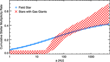
Figure 3. Comparison of the cumulative stellar multiplicity rate between field stars in the solar neighborhood (blue) and gas giant planet host stars (red). Hatched regions represent 1σ uncertainty regions. The stellar multiplicity rate for planet host stars is  % within 20 AU. In comparison, the stellar multiplicity rate is 18% ± 2% for the control sample. The stellar multiplicity rate for planet host star is 34% ± 8% for separations between 20 and 200 AU, which is higher than the control sample at 12% ± 2%. Beyond 200 AU, stellar multiplicity rates are comparable between planet host stars and the control sample.
Download figure:
Standard image High-resolution imageThe stellar MR for planet host stars is consistent with zero and stays flat at  % for stellar separations smaller than 20 AU. For 20 AU
  200 AU, the stellar MR is 34% ± 8%. The increase of the cumulative stellar MR from [0–20] to [20–200] AU is much faster than the control sample whose cumulative stellar MR changes from 18% to 30%. Beyond 200 AU, the stellar MR for planet host stars is higher than that for the control sample, but they are consistent within measurement uncertainty. The slopes for the cumulative stellar MR change are similar between planet host stars and the control sample.
7. DISCUSSION
7.1. Interpretation of the Stellar Multiplicity of Stars With Gas Giant Planets
According to Figure 3, there may be three stellar separation ranges in which stellar companions affect gas giant giants formation and evolution differently. For stellar separations smaller than 20 AU, planet formation is suppressed. No stellar companion has been found within 20 AU for Kepler stars with gas giant planets. This leads to a zero stellar multiplicity (0 %) that is significantly lower than that for the control sample (18% ± 2%).
For separations between 20 and 200 AU, we notice a drastic increase of the cumulative stellar MR for planet host stars. In contrast to the stellar MR of 12% ± 2% in this separation range for the control sample, the stellar MR is 34% ± 8% for planet host stars. The higher stellar MR for planet host stars suggests that stellar companions in this separation range play an important role in gas giant planet migration, e.g., via the Lidov–Kozai mechanism. Therefore, for 20 AU  200 AU, the role of stellar companions in planet migration is more important than their role in suppressing planet formation. However, there may be a caveat asserting the role of stellar companions in planet migration. The search completeness is ∼30%–50% between 20 and 200 AU (Figure 2), which is the lowest in the
  parameter space. Therefore, the stellar MR in this separation range is the most uncertain.
For separation beyond 200 AU, the stellar MR for planet host stars is comparable to that for the control sample, which indicates that gas giant planet formation and evolution is not significantly affected by a stellar companion.
7.2. Comparison to Stars with Small Planets
Wang et al. (2014a) measured the cumulative stellar MR for a sample of planet host stars. This sample is dominated by stars with smaller planets, 43 out 56 stars have only transiting planets that are smaller than 3.8  . We compare the stellar MRs from Wang et al. (2014a) and this work, which focuses on gas giant planet host stars. While they are qualitatively identical, the characteristic separations are different. For example, the stellar MR for small planet host stars intersects with control sample at ∼1500 AU whereas the intersection takes place at ∼100 AU for gas giant planets. The effective range of a stellar companion is an order of magnitude larger for small planets than for large planets: smaller planets are more prone to the influence of a stellar companion.
There may be several explanations. First, in a multi-planet system, the timescale for pericenter precession and nodal precession increases with decreasing planet mass (Takeda et al. 2008). For planet systems of the same orbital configurations, the Kozai timescale is more likely to be shorter than the timescale for pericenter precession and nodal precession for smaller planets, which makes these systems dominated by the Kozai effect due to the stellar companion. Therefore, smaller planets are more prone to the influence of a distant stellar companion because of a weaker planet–planet dynamical coupling. Second, for planet systems with both small and large planets, dynamical interaction between these two types of planets tend to eject more small planets than large planets (J. W. Xie et al. 2015, in preparation). In the presence of stellar companions, the dynamical interaction becomes more frequent and thus leads to higher loss of small planets.
7.3. Correlation between Stellar Companion Properties and Planet Properties
Planet formation is subject to the influence of stellar companions. Therefore, planets with different properties (e.g., orbital period and planet radius) may be a result of different properties of stellar companions. Here, we study whether the difference in stellar companions results in the difference of planet properties.
For properties of stellar companions, we focus on their differential magnitudes (Δ Mag). Since the majority (51 out of 59) of detected stellar companions have differential magnitudes in the K band, we use those. For those whose K band differential magnitudes are not available, we do not use them in the following analysis.
To find evidence that stellar companion properties affect planet properties, we adopt a K-S-test-based method that has been used to search for different populations divided by a parameter (Buchhave et al. 2014; Quinn et al. 2014). The method is described as follows. We choose a value x for a planet property parameter. The value divides the sample into two sub-samples. We then compare the stellar companion properties of two sub-samples with the K-S test. The p value of the K-S test is recorded. By varying x and repeating the K-S test, we obtain a function p(x). If there are certain x values that result in significant difference between two sub-samples, these values may represent characteristic values that divide different planet populations. These populations are a result of different properties of stellar companions. Because not all stellar companions are physically associated, we need to account for the effect of inclusion of optical double/multiples. The uncertainty due to this effect is addressed in a Monto Carlo simulation. In each trial, we draw a subset of detected stellar companions based on the probability of their physical association. We apply the K-S-test-based method to the subset and record p(x). We repeat the process for 1000 times and find the median and confidence intervals at different levels.
Figure 4 shows the p value in K-S test as a function of planet orbital period. The K-S test compares the Δ Mag of two sub-samples divided by orbital period. The K-S test-based method suggests that there may be three different populations of gas giant planets. We caution that this finding is not conclusive at this stage given small number statistics. If using p = 0.05 as a threshold, the dividing orbital periods are ∼10 and ∼70 days. The p-value dip at P ∼ 10 days is broad extending from 7 to 22 days. Hereafter we use P ∼ 10 days as a representative value. The stellar properties of these three populations may be distinctively different. Figure 5 shows the Δ Mag distribution. Stars with gas giant planets with  days tend to have more stellar companions with small differential magnitudes (Δ Mag > 2). In comparison, Δ Mag for stars with gas giant planets with
  days tend to be fainter but peak at Δ Mag ∼ 3. However, the peak may be due to a lack of sensitivity for fainter stellar companions. The Δ Mag for stars with gas giant planets with
  days lies in between the previous two populations.
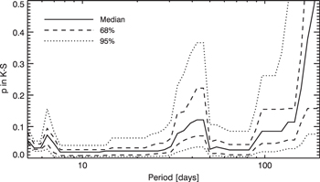
Figure 4. Results of K-S tests for the null hypothesis that stars with shorter-period and longer-period gas giant planets have stellar companions with similar distribution of differential magnitude. At each dividing period, we conduct a Monte Carlo simulation and show the median (solid) and 68% (dashed) and 95% (dotted) confidence intervals. There may be three populations of gas giant planets whose formation and evolution are influenced differently by their stellar companions. The dividing periods for these populations are ∼10 and ∼70 days.
Download figure:
Standard image High-resolution image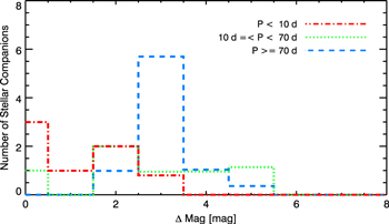
Figure 5. Distribution of differential magnitude for stellar companions. For stars with short-period gas giant planets ( days), stellar companions tend to be bright with small differential magnitudes. For stars with gas giant planets with
  days, the differential magnitudes of their stellar companions tend to be fainter than the short-period counterparts. There is a peak at ∼3.0 mag, but it may be due to a lack of sensitivity for fainter stellar companions.
Download figure:
Standard image High-resolution image
We check whether the finding of three distinct populations is prone to inclusion of false positives. One major cause of a false positive is underestimation of the radius due to flux contamination. Horch et al. (2014) estimate the effect as a function of ΔMag in the Kepler band in two scenarios: an object transiting a primary star and an object transiting a secondary star. After applying their calculation, there are five KOIs that could be false positives. All the potential false positives are for the scenarios in which an object is transiting a secondary star. These KOIs are KOI-17, KOI-375, KOI-633, KOI-2672, and KOI-3678. Among them, KOI-17, also known as Kepler-6, has been confirmed (Dunham et al. 2010). KOI-2672 is a system with multiple transiting planet candidates, so the false positive probability is low (Lissauer et al. 2012). The stellar companions for KOI-375, KOI-633, and KOI-3678 are only detected in the K band and have differential magnitudes of 3.3, 3.9, and 3.3 mag. If physically associated, the K band differential magnitudes would put the stellar companions in the range of early-type M dwarfs. Such low-mass stars are less likely to harbor gas giant planets, which makes the scenario in which an object transits the secondary star less probable. Given the false positive rate of ∼20% (Fressin et al. 2013), there would be at most one KOI that is a false positive, which will not significantly reduce the peak seen in Figure 5. However, we must caution again that the three-population hypothesis is preliminary and remains to stand the test of more observations and a larger sample.
7.4. Comparison to Other Results
The stellar MR of planet host stars has been a research interest for a number of works (see Section 1 for references). All previous results concerning the Kepler sample were for small planet host stars. This is because Kepler discoveries are dominated by small planets and these planets are of great interest for potential habitable worlds. Ngo et al. (2015) used a sample of stars with gas giant planets that were discovered by ground-based RV and transiting surveys. In their "Friends of HJs" project, they found that the stellar multiplicity for 50 stars with HJs is 48% ± 9% for the stellar separation range of 50–2000 AU. We have 28 HJs in our sample, the stellar MR we find for these separations is 25% ± 20%. However, if considering separations smaller than 50 AU, the stellar MR within 2000 AU is 51% ± 13%. The significant difference is due to the drastic change of stellar MR between 20 and 200 AU (Figure 3).
In Section 7.3, we suggest that the stellar companions around HJ host stars are on average brighter than stellar companions around stars hosting longer-period gas giant planets (Figure 5). In our sample, all stellar companions around HJ host stars have K band differential magnitudes smaller than 2.5 with one exception of KOI-17 (Δ Mag = 3.8 mag). The trend is absent in Ngo et al. (2015). None of their detected stellar companions have differential magnitudes smaller than 2.5 mag. One explanation is that they focus on stars with HJs discovered by ground-based RV and transiting surveys. In these surveys, a strong bias against MSS exists in the target selection and follow-up observations. The fact that Ngo et al. (2015) detected many fainter stellar companions suggests that there may be a missing population of HJ systems in equal-mass binary systems. Recent discovery of HJs in WASP-94 AB system is one example of such systems (Neveu-VanMalle et al. 2014).
Law et al. (2014) observed 715 KOIs using the Robo-AO system, they found that stars hosting short-period ( days) giant planets are 2–3 times more likely to have stellar companions than their longer-period counterparts. For our sample, we have 32 giant planets with periods shorter than 15 days. When comparing the stellar MR for stars hosting short-period planets and the rest of our sample, we do not find a significant difference. In fact, the stellar MRs for the stars with short-period planets, stars with planets with
  days, and the entire sample are all ∼50% within 5000 AU. For stars with short-period planets, they tend to have brighter stellar companions, which are easier for Robo-AO to detect. For stars with planets with longer periods, their stellar companions tend to be fainter with differential magnitudes peaking at Δ Mag = 3.0 in K band. These faint stellar companions are 1–2 mag fainter in the visible bands at which Robo-AO operates. Thus they are likely to be missed by Robo-AO given the detection limits are ∼4–5 mag in r and i band for the median performance. The portion of fainter stellar companions missing in the Robo-AO survey may explain their finding that stars hosting short-period (
 days) giant planets are 2–3 times more likely to have stellar companions. Therefore, we suspect that the finding in Law et al. (2014) may be caused by a lack of sensitivity to faint stellar companions.
Jang-Condell (2015) quantified planet formation efficiency in close binaries. The paper gave an empirical equation of gas giant planet formation efficiency as a function of primary star mass, mass ratio, binary separation, and binary orbital eccentricity. Our finding of a suppressive planet formation within 20 AU is consistent with the conclusion in Jang-Condell (2015). However, Jang-Condell (2015) predicted that gas giant planets in close binaries with separations smaller than 20 AU are not entirely impossible. In comparison, there is no such planetary system in our sample. The closest stellar companion we have detected is at 40.3 AU projected separation. There are several other planetary systems in close binaries detected by the RV technique, such as γ Cep and HD 41004, but none of them has a binary separation smaller than 20 AU. The contrast between observations and theoretical predictions implies that a close stellar companion not only decreases the planet formation efficiency but also negatively influences planet evolution. Jang-Condell (2015) also discussed the effect of mass ratio on planet formation. While we found the tentative correlation between HJ occurrence and equal-brightness stellar companion, it is difficult to make a direct comparison because Jang-Condell (2015) focused on stellar companions with separations smaller than 100 AU whereas all but one companions in our study have separations larger than 100 AU.
8. SUMMARY
We select a sample of 84 KOIs with 97 gas giant planets to study the influence of stellar companions on planet formation. We obtain AO images for 60 KOIs with two instruments: PHARO at the Palomar 200 inch telescope and NIRC2 at the Keck II telescope. For the rest of the sample, we use AO images available from the CFOP database. In total, we have detected 59 stellar companions around 40 KOIs.
Since some of the detected stellar companions are not physically associated with the KOIs, we develop two methods of testing the physical association. The first method makes use of the color information. For stellar companions with detections in multiple filters, we estimate their masses and absolute magnitudes based on their colors. Their distances can be estimated from the absolute magnitudes, apparent magnitudes, and extinctions. By comparing the distances of stellar companions and the KOIs, we can test their physical association. The second method is based on the statistics of the galactic stellar population. For stellar companions that are detected in only one filter, the color information is missing. Instead, we run a galactic stellar population model to simulate the Kepler field. With the results, we estimate the relative probability of gravitationally bound stellar companions and optical doubles/multiples. Then we can calculate the probability of physical association as a function of angular separation and differential magnitude of a stellar companion. With these two methods of testing physical association, we can effectively exclude the effect of foreground and background stars on stellar MR.
We find that the stellar MR for planet host stars is  % within 20 AU. In comparison, the stellar MR is 18% ± 2% for the control sample, i.e., field stars in the solar neighborhood. The deficiency of stellar companions for planet host stars indicates that gas giant planet formation is suppressed by stellar companions within 20 AU. The stellar MR for planet host stars is 34% ± 8% for separations between 20 and 200 AU, which is higher than the control sample at 12% ± 2%. This suggests that stellar companions in this separation range play an important role in gas giant planet migration. Beyond 200 AU, stellar MRs are comparable between planet host stars and the control sample.
We explore whether stellar companions of different properties lead to different planet properties. We find evidence of three distinct populations of gas giant planets. They are separated by two characteristic orbital periods, 10 and 70 days. The stellar companions around stars with each planet population have different differential magnitude distributions. For example, stars with HJs ( days) tend to have bright stellar companions with K band differential magnitudes smaller than 2 mag. Stars with gas giant planets with
  days tend to have stellar companions whose differential magnitudes peak at ∼3.0 mag in the K band, which correspond to early type M dwarf companions. We emphasize that the three-population hypothesis is still tentative, and more follow-up observations are needed to either support or disprove it.
If the three-population hypothesis survives future tests, it may have significant implications on gas giant planet formation and evolution. First, the migration of gas giant planets may be dependent upon the mass of a stellar companion. The majority of gas giant planets in our sample cannot form in situ because of a lack of building and accreting materials. They must migrate in via some mechanisms. The migration mechanisms could be the same for different planet populations, e.g., the Lidov–Kozai mechanism. Or the migration mechanisms could be different, e.g., the Lidov–Kozai mechanism for HJs and in-disk migration for longer-period planets. In either case, the migration mechanisms have to be consistent with the observed mass-dependency of stellar companions.
Second, if HJs tend to be preferentially found in binary star systems with similar magnitudes, this population of HJs has been neglected because of the concern with flux contamination. The HJs in WASP-94 AB (Neveu-VanMalle et al. 2014) and Kepler-13 AB (Szabó et al. 2011; Mazeh et al. 2012; Johnson et al. 2014; Shporer et al. 2014) systems may be the tip of the iceberg for this population. Surveys that do not bias against MSS can constrain the HJ occurrence rate in binary star systems with similar magnitudes. Current and future space missions for transiting planets, e.g., the K2 mission (Howell et al. 2014) and the TESS mission (Ricker et al. 2014), may serve that purpose. In fact, the transiting signal of HJs in binary stars may already exist in ground-based transiting surveys. In addition, AO-fed spectrographs will play an important role in validating or confirming HJs in binary stars (e.g., Crepp 2014).
The authors thank the anonymous referee whose comments and suggestions greatly improved the paper. The authors would like to thank the telescope operators and supporting astronomers at the Palomar Observatory and the Keck Observatory. Some of the data presented herein were obtained at the W. M. Keck Observatory, which is operated as a scientific partnership among the California Institute of Technology, the University of California, and the National Aeronautics and Space Administration. The Observatory was made possible by the generous financial support of the W. M. Keck Foundation. The research is made possible by the data from the Kepler Community Follow-up Observing Program (CFOP). The authors acknowledge all the CFOP users who uploaded the AO and RV data used in the paper. This research has made use of the NASA Exoplanet Archive, which is operated by the California Institute of Technology, under contract with the National Aeronautics and Space Administration under the Exoplanet Exploration Program. J.W.X. acknowledges support from the National Natural Science Foundation of China (Grant No. 11333002 and 11403012), the Key Development Program of Basic Research of China (973 program, Grant No. 2013CB834900) and the Foundation for the Author of National Excellent Doctoral Dissertation (FANEDD) of PR China. J.W. acknowledges the travel fund from the Key Laboratory of Modern Astronomy and Astrophysics (Nanjing University). We thank Eric Ford for insightful comments on interpreting the stellar multiplicity rate of planet host stars.
Footnotes
- 4
- 5
- 6
- 7