


ABSTRACT
Zank et al. developed a turbulence transport model for low-frequency incompressible magnetohydrodynamic (MHD) turbulence in inhomogeneous flows in terms of the energy corresponding to forward and backward propagating modes, the residual energy, the correlation lengths corresponding to forward and backward propagating modes, and the correlation length of the residual energy. We apply the Zank et al. model to the super-Alfvénic solar wind i.e.,  and solve the coupled equations for two cases, the first being the heliosphere from 0.29 to 5 AU with and without the Alfvén velocity, and the second being the "entire" heliosphere from 0.29 to 100 AU in the absence of the Alfvén velocity. The model shows that (1) shear driving is responsible for the in situ generation of backward propagating modes, (2) the inclusion of the background magnetic field modifies the transport of turbulence in the inner heliosphere, (3) the correlation lengths of forward and backward propagating modes are almost equal beyond ∼30 AU, and (4) the fluctuating magnetic and kinetic energies in MHD turbulence are in approximate equipartition beyond ∼30 AU. A comparison of the model results with observations for the two cases shows that the model reproduces the observations quite well from 0.29 to 5 AU. The outer heliosphere (
 AU) observations are well described by the model. The temporal and latitudinal dependence of the observations makes a detailed comparison difficult but the overall trends are well captured by the models. We conclude that the results are a reasonable validation of the Zank et al. model for the super-Alfvénic solar wind.
Export citation and abstract BibTeX RIS
1. INTRODUCTION
Magnetized turbulence is commonly present throughout the solar wind, from the solar corona to the heliopause and possibly even in the interstellar medium. The solar wind has been used to study magnetohydrodynamic (MHD) turbulence from the beginning of the space age (Coleman 1968; Belcher & Davis 1971; Bavassano et al. 1982; Goldstein 1995; Goldstein et al. 1995b; Tu & Marsch 1995; Bruno & Carbone 2005, 2013). Our understanding of solar wind turbulence has increased rapidly with the increasing availability of measured data from several spacecraft. A surprising characteristic of the solar wind is the observed non-adiabatic solar wind temperature profile (Gazis et al. 1994; Freeman 1988; Williams et al. 1995; Matthaeus et al. 1999b; Smith et al. 2001, 2006a, 2006b; Isenberg et al. 2003; Isenberg 2005; Breech et al. 2008; Isenberg et al. 2010; Ng et al. 2010; Oughton et al. 2011; Usmanov et al. 2011), i.e., the temperature does not follow an adiabatic cooling law  , where r is heliocentric distance. Beyond 20–25 AU, the temperature begins to increase (Williams et al. 1995; Richardson 2010), although some modest decrease can occur again between 35–50 AU (Isenberg et al. 2010). The non-adiabatic temperature profile of the solar wind is now generally attributed to the dissipation of turbulence, whether pre-existing or generated in situ by a variety of sources and mechanisms. Besides the heating of the solar wind by thermal dissipation, MHD turbulence is thought to be fundamental to several other dynamical processes in the solar wind. These include the scattering of solar energetic particles in the solar wind (Li et al. 2003; Zank et al. 2007), and the heating of the solar corona to millions of degree Kelvin and the generation of the fast solar wind from the open field region of the heated solar corona (Leer et al. 1982; Matthaeus et al. 1999a; Dmitruk et al. 2001, 2002; Oughton et al. 2001; Suzuki & Inutsuka 2005, 2006; Verdini et al. 2010; van Ballegooijen et al. 2011; Asgari-Targhi et al. 2013; Lionello et al. 2014; Matsumoto & Suzuki 2014). Several models have been proposed to describe the heating and acceleration mechanisms of the solar corona and solar wind, with varying degrees of success, but none are universally accepted. However, there are two leading candidates, the ion cyclotron heating and the turbulence cascade models, both of which depend on the presence of upwardly propagating Alfvénic or magnetized fluctuations.
Coleman (1968) and Belcher & Davis (1971) studied MHD fluctuations in the solar wind observationally, and observed that there exist both MHD waves (Belcher & Davis 1971) and MHD turbulence (Coleman 1968). In most cases, the fast and slow MHD modes waves are dissipated rapidly. Near the Sun, fluctuations of the velocity and magnetic field are often highly correlated (Coleman 1967; Belcher & Davis 1971), are associated with MHD Alfvén waves, and possess a high degree of Alfvénicity, which decreases with increasing heliocentric distance (Roberts et al. 1987a, 1987b). The correlation can be an intrinsic property of the source, or it can be created through nonlinear interactions between two oppositely propagating modes (see also Grappin et al. 1982). Based on their observational studies Belcher et al. (1969) and Belcher & Davis (1971) introduced the idea that solar wind fluctuations may be regarded as a superposition of linear MHD waves, specifically Alfvén waves. As the solar wind flows outward, turbulence generated in the solar wind cascades energy from larger scales to smaller scales. The spectra of such fluctuations usually exhibit a Kolmogorov-type scaling in the inertial range with an index of  in a wave number space (Matthaeus & Goldstein 1982; Bale et al. 2005; Alexandrova et al. 2009), with approximate equipartition between the fluctuating kinetic and magnetic energy. An Iroshnikov-Kraichnan-type of scaling,
  (Iroshnikov 1964; Grappin et al. 1982; Perez & Boldyrev 2008), where k is a wave number, can also be observed in the solar wind (Podesta et al. 2007). Grappin et al. (1983) have shown that the power law can depart from a 3/2 index when
  and
and  are correlated.
There exist both inward/backward and outward/forward fluctuations in the solar wind. The fluctuations are called inward/backward if they propagate anti-parallel to the outwardly directed interplanetary magnetic field (IMF) with respect to the Sun, otherwise the fluctuations are called outward/forward. In the limit of quasi-incompressible MHD, adopted here, the nonlinear interaction between forward and backward propagating wave leads to the transfer of energy from larger scales to smaller scales (Howes et al. 2008), which eventually is dissipated as heat (Marino et al. 2008). Dissipation of turbulence therefore leads to solar wind heating. Since only forward propagating modes escape from the sub-Alfvénic region, backward propagating modes observed in the super-Alfvénic wind are not of solar origin and must be created in situ by local physical processes. The energy difference associated with these forward and backward propagating modes is known as the cross helicity. It can be negative, positive, or zero. Positive cross helicity indicates the dominance of forward propagating modes, and negative indicates dominant backward propagating modes. In the case of equal energy in forward and backward propagating modes, the cross helicity is zero. The cross helicity decreases monotonically with increasing heliocentric distance (Matthaeus et al. 1994, 2004; Breech et al. 2005). The cross helicity does not identify whether the energy resides in the magnetic field or velocity field. The "residual energy" or "energy difference" (i.e., difference between fluctuations in the kinetic and magnetic energy) measures this property, and is therefore another important quantity (Grappin et al. 1983; Müller & Grappin 2005). Similarly, the residual energy can also be negative, positive, or zero. Negative residual energy indicates the dominance of magnetic energy in MHD fluctuations, and positive indicates the dominance of kinetic energy, while zero residual energy indicates equipartition between the fluctuating kinetic and magnetic energy. Theoretical and simulation results show that the residual energy is mostly negative (Grappin et al. 1983; Matthaeus et al. 1994; Müller & Grappin 2005; Yokoi & Hamba 2007; Wang et al. 2011; Chen et al. 2013). It is also observed that at smaller scales the magnetic energy is dominant (Bruno et al. 1985; Roberts et al. 1987a, 1987b), and at larger-scales the kinetic energy dominates. The magnetic field spectrum is observed to be steeper than the velocity spectrum in the inertial range (Podesta et al. 2007), and the residual energy decays as  , where
  is a wave number perpendicular to the background magnetic field (Grappin et al. 1983; Müller & Grappin 2005; Boldyrev et al. 2011). The evolution of these various quantities has not been investigated theoretically as a fully closed system. In this paper, we solve numerically the transport model for low-frequency MHD turbulence introduced by Zank et al. (2012a). The Zank et al. (2012a) model describes the evolution of the energy in forward and backward modes, the cross helicity, the residual energy, and the associated correlation lengths.
During the expansion of the solar wind, fluctuations in the solar wind velocity, solar wind density (Bellamy et al. 2005; Hunana & Zank 2010; Zank et al. 2012b), and magnetic field (Zank et al. 1996; Matthaeus et al. 1999b; Smith et al. 2001) are generated in situ and transported throughout the heliosphere. The fluctuations are highly Alfvénic near the Sun, which despite exhibiting many characteristics of fully developed turbulence, has nonetheless been described traditionally using a linearized wave description, or WKB theory. WKB theory shows that the variance of the fluctuating magnetic field  decays as
  . However, WKB theory being a linear wave theory can not explain the radial evolution of MHD turbulence related quantities in the heliosphere (Bavassano et al. 1982; Roberts et al. 1987b; Zank et al. 1996; Matthaeus et al. 1999b; Smith et al. 2001). Zank et al. (1996) first proposed a coupled turbulence transport model of the fluctuating magnetic energy density Eb and the correlation length l to address the problems inherent in the WKB model. Related analysis were presented by Matthaeus et al. (1999b) and Smith et al. (2001), and moreover they included heating of the plasma due to the dissipation of turbulence. The Zank et al. (1996) model cannot be applied within 1 AU since it makes several assumptions that are not reasonable for the inner heliosphere. The turbulence transport model was further developed by Matthaeus et al. (2004), and Breech et al. (2005, 2008), in that they included the cross helicity, which was neglected by Zank et al. (1996). These models do not, however, address either the residual energy or the role of the Alfvén velocity, both of which are important to the corona and inner heliosphere. Motivated by these shortcomings, Zank et al. (2012a) extended the Zank et al. (1996) model to incorporate cross helicity, residual energy, Alfvén velocity, and various correlation lengths. Therefore, the Zank et al. (2012a) model is an important extension to the previous models describing the transport of turbulence in the solar wind. In this paper we introduce source terms that were not discussed in Zank et al. (2012a), and solve the complete steady state turbulence transport model in spherical coordinates, neglecting θ and ϕ coordinates, as was done in Zank et al. (1996), Matthaeus et al. (1999b, 2004), Smith et al. (2001), and Breech et al. (2005, 2008). The 1D model addresses only radial dependence and neglects the effects of the latitudinal and longitudinal dependence of the large-scale solar wind in the transport of turbulence. These effects are likely to be important when considering the solar wind during solar minimum, where a distinct high speed polar wind and a low speed ecliptic wind are present. However, by restricting our models to either the ecliptic or polar regions, a 1D turbulence transport model should be adequate. During solar maximum the sources of turbulence are different from solar minimum and possibly time-dependent. We have shown in Adhikari et al. (2014) that a steady-state 1D turbulence transport model well describes the corresponding time-dependent solutions. A more technical complication distinguishing the 3D from the 1D models is in the inclusion of the Alfvén velocity. The inclusion of Alfvén velocity renders the turbulence transport equation fundamentally multidimensional. By using the assumption that
  or considering any region of radial IMF, we can recover a 1D model. This is discussed further below. Finally, we compare our numerical solutions with observations. By doing so, we indirectly validate the various closure assumptions made in developing the turbulence formalism of Zank et al. (2012a).
2. BACKGROUND
We adopt a mean field decomposition to derive equations that describe the evolution of turbulence in the inhomogeneous solar wind. The flow velocity  and the magnetic field
  are written in terms of the mean and fluctuating fields as,
  ;
;  , where
  and
and  are the mean fields, and
  and
and  are the fluctuating fields. The fluctuating fields possess many features expected of fully developed MHD turbulence. The combination of the small scale fluctuating fields can be defined in terms of the Elsässer variables,
  (Elsässer 1950), where ρ is the solar wind density. The Elsässer variables
  are functions of both large scales (e.g., background solar wind scales) and small scales (e.g., turbulence scales), and are important parameters for describing the MHD turbulence. The averaging procedure ensures that the fluctuating fields average to zero such that
  and
and  .
.
The two scale-separated MHD equations describing the evolution and transport of arbitrary amplitude fluctuations  and
and  about the inhomogeneous mean velocity field
  and magnetic field
  , in terms of the Elsässer variables can be expressed as (Marsch & Tu 1989; Zhou & Matthaeus 1990a, 1990b)
where I is the identity matrix, and  (Zank et al. 2012a) is a nonlinear term denoting the nonlinear interaction between forward and backward propagating modes or between counter-propagating Alfvén waves packets. The turbulence is strong if the wave packets are deformed significantly in one interaction (or one crossing time), otherwise the turbulence is weak. Weak turbulence has been studied using perturbation theory by Galtier et al. (2000, 2002; see also Sridhar & Goldreich 1994; Ng & Bhattacharjee 1996). Similarly, strong Alfvénic turbulence has been studied by Goldreich & Sridhar (1995). The nonlinear term always vanishes when
  or
or  , and the incompressible equation reduces to a set of linear wave equations (Grappin et al. 1982). The parameter
  is a source term that is related to either stream-shear interactions or pickup ions, and
  is the large scale Alfvén velocity. Here
  (
( ) represents the inward (outward) propagating modes with respect to the outward IMF field orientation. Thus,
  is anti-parallel to the large scale magnetic field
  , and
, and  is parallel to
  .
.
Equation (1) is derived from the well-known form of the incompressible MHD equations when expressed in terms of the Elsässer variables (Marsch & Tu 1989; Zhou & Matthaeus 1990a, 1990b). By taking moments of Equation (1) and introducing several assumptions, such as zero cross helicity and neglecting the Alfvén velocity, Zank et al. (1996) developed a simple turbulence transport model to describe the evolution of the fluctuating magnetic energy density ( ) and correlation length (l) in the outer heliosphere beyond 1–2 AU. However, the model neglected the Alfvén velocity and assumed zero cross helicity, and hence cannot be applied to the inner heliosphere where the cross helicity is observed to be non-zero. The inclusion of dissipative heating of the background turbulence into the model by Matthaeus et al. (1999b) and the detailed observational analysis by Smith et al. (2001) provided considerable support for the Zank et al. (1996) model, at least for the outer heliosphere. Matthaeus et al. (2004) investigated the radial dependence of the cross helicity and showed that the cross helicity decreases with increasing heliocentric distance and is approximately zero from beyond ∼30 AU. This result indicates that an approximately equal number of forward and backward propagating modes are present beyond 30 AU (see also Breech et al. 2005). Furthermore, the value of the cross helicity also depends on helio-latitude (Breech et al. 2005), being larger at higher latitude (Goldstein et al. 1995a; Malara et al. 2000; Grappin 2002) and smaller at lower latitude (Roberts et al. 1992). Turbulence generated by shear associated with stream interactions, stronger at lower latitude and weaker at higher latitude, is thought to be responsible for the decrease in cross helicity (Roberts et al. 1992). The Breech et al. (2008) model was developed to include the cross helicity, which was done by applying a similar formalism as introduced by Zank et al. (1996). The Breech et al. (2008) model partially addresses the transport of turbulence from the inner to the outer heliosphere, but explicitly neglects the residual energy and assumes
  . Zank et al. (2012a) developed a more general turbulence transport model that does not involve the simplifying assumptions of Zank et al. (1996) and addresses the limitations of Breech et al. (2008). We note that Zank et al. (2012a), like Breech et al. (2008), introduce several assumptions to affect closure of the moments derived from Equation (1). The dissipation terms for the total energy and cross helicity derived in the Zank et al. model are based on an isotropic assumption, consistent with the conservation of the so-called "rugged invariants" (Matthaeus & Goldstein 1982). The dissipation term for the residual energy is less robust. In general, the modeling of the dissipation terms are approximated and complicated. Thus, the model has to be validated, and the validity of these assumptions can only be addressed properly by comparing model solutions to observations. Accordingly, we solve below the Zank et al. model for the super-Alfvénic solar wind and compare our solutions to a suite of observations. The Zank et al. model in terms of
  and
and  with
with  and b = 0, is given by


where f and g denote the energy in backward and forward propagating modes, respectively,  is the residual energy,
  and
and  are the correlation lengths of backward and forward propagating modes, respectively, and
  is the correlation length of the residual energy. The dissipation term for the evolution of ED, the first term on the right-hand side (rhs) of Equation (4), is similar to that introduced by Dosch et al. (2013), except that we do not assume
  . Since we use a different dissipation term for ED than used by Zank et al. (2012a), the first term on the rhs of Equation (7) is also different than the first two terms on the rhs of Equation (46) of Zank et al. (2012a). The angle bracketed terms
  and
and  are the sources of turbulence, which we discuss later. The parameter
  corresponds to the shear mixing term, and is neglected by choosing
  . The transport models of Zank et al. (2012a) are complex and contain much more information than previous models e.g., Matthaeus et al. (1994, 2004), Zank et al. (1996), and Breech et al. (2005, 2008). The model shows for example that backward propagating modes are created by the reflection of forward propagating modes, which may be important in other environments such as the solar corona. The Zank et al. (2012a) model reduces to the well-known WKB model in the absence of Alfvén velocity, mixing, dissipation, and source terms (Appendix D of Zank et al. 2012a).
The dissipation of turbulence is thought to be responsible for heating the solar wind (Williams et al. 1995; Matthaeus et al. 1999b; Smith et al. 2001, 2006a, 2006b; Isenberg et al. 2003, 2010; Isenberg 2005; Breech et al. 2008; Oughton et al. 2011; Usmanov et al. 2011), and considering the dissipation terms of the f, g, and ED transport equations, the equation for the solar wind temperature T can be written in a form similar to that of Smith et al. (2001, 2006a, 2006b), Isenberg et al. (2003), and Isenberg (2005) as
where  is the adiabatic index, mp is the proton mass, kB is the Boltzmann constant, and α is the von Kármán-Taylor constant. We chose
  (Smith et al. 2001). The rhs of Equation (8) is a heating term for the solar wind, in the absence of which the solar wind temperature profile is adiabatic. The total turbulent energy ET, the cross helicity EC, the fluctuating magnetic energy density Eb, and the Alfvén ratio rA can be calculated by using the following relations (Zank et al. 2012a),


Several previous work have studied these quantities observationally and theoretically. Matthaeus et al. (1994) investigated the evolution of the energy corresponding to forward and backward propagating modes, the cross helicity, the residual energy, and the correlation length from almost 0.05–2 AU, but did not consider any kind of turbulence source. Matthaeus et al. (2004) and Breech et al. (2005) investigated the evolution of the cross helicity from 0.3 to 100 AU. Similarly, Breech et al. (2008) studied the total turbulent energy, the solar wind temperature, the cross helicity, and the correlation length from 0.3 to 100 AU. Zank et al. (1996), and Adhikari et al. (2014) studied the fluctuating magnetic energy density from 1 to 80 AU. All these models describe the transport of various turbulent quantities in the super-Alfvénic flow, sometimes quite successfully. In this paper, we investigate a more complete set of solar wind turbulence properties from 0.29 to 5 AU with and without including the Alfvén velocity, and from 0.29 to 100 AU after neglecting the Alfvén velocity. Retaining the Alfvén velocity in the model allows us to more carefully quantify the effect of assuming  in the super-Alfvénic flow. We also investigate the theoretical and observational correlation lengths for each energy mode.
3. SOURCE OF TURBULENCE
There are three primary sources of turbulence in the heliosphere, and are specific to spatial locations in the heliosphere. The sources may be characterized as (1) turbulence driven by shear due to the interaction between fast and slow solar wind streams (Coleman 1968; Roberts et al. 1992), (2) compressional sources of turbulence due to stream-stream interactions and shock waves (Whang 1991), and (3) turbulence due to pickup ions created by charge exchange between solar wind protons and interstellar neutral hydrogen (Williams & Zank 1994). Depending on location as well as properties, the sources can be divided into two groups.
(1) Stream shear and shock wave driven turbulence: the velocity shear is an important indicator in the evolution of solar wind fluctuations. The expressions for these sources can be written similarly to that of Zank et al. (1996),


where the parameters  and
and  are the strength of the shear interaction for backward and forward propagating modes, respectively. Also,
  (=350 km s−1) is the difference between the fast and slow solar wind speeds. The rate of shear driving is assumed to be equal for forward and backward propagating modes i.e.,
  . Furthermore, Equations (13)–(15) represent the shear source of turbulence for backward, forward, and the residual energy, respectively. Similarly, the source terms due to the presence of shocks, following the approach of Zank et al. (1996), are


where  and
and  are the shock driving for backward and forward propagating modes, respectively, and
  is the difference between the upstream and downstream speed of the shock.
(2) Pickup ion driven turbulence in the outer heliosphere: as pickup ions beyond the ionization cavity isotropize, they generate turbulence in the outer heliosphere. In the case of  (
( is the velocity parallel to the IMF), the wave energy generated by pickup ions is shared equally to both forward and backward propagating modes (Williams & Zank 1994). If
  instead, more
  waves are excited and if
  more
more  waves are excited. Since the radial solar wind flow is primarily orthogonal to the mean magnetic field, the PUI source of turbulence is similar to that used by Zank et al. (1996), Breech et al. (2008), Isenberg et al. (2003) and Isenberg (2005), and is given by


Here,  and
and  , and are functions of
  , which determines the fraction of pickup ion energy transferred into excited waves (Isenberg et al. 2003; Isenberg 2005), and
  . Equations (19) and (20) represent the pickup ion source for backward and forward propagating modes, respectively. The parameter
  cm−3 is the number density of interstellar neutrals,
  s is the neutral ionization time at 1 AU, ψ is the angle between the observation point and the upstream direction,
  AU and λ is the ionization cavity length scale. Also,
  cm−3, and VA = 50 km s−1. Equation (21) is the pickup ion source of turbulence for the residual energy, which is zero since it is assumed that only Alfvénic fluctuations are generated.
4. METHOD
The 1D steady state form of the seven coupled transport Equations (2)–(8) are solved in a spherical coordinate system, neglecting the θ and ϕ components. We use Runge–Kutta 4 to solve the model equations numerically. We solve the model in the super-Alfvénic flow region where the solar wind speed is almost constant. By assuming a spherically symmetric flow, we have  =
=  , where U0 = 400 km s−1 is the solar wind speed. The Alfvén velocity related to the IMF can be given as (Parker's model, Parker 1958)
where  (
( km is a solar radius),
  km s−1 is the Alfvén speed,
  rad s−1 is the angular speed of the Sun, and θ denotes colatitude with respect to solar rotation. We chose
  i.e., the ecliptic plane. The inner boundary conditions for the turbulence variables at 0.29 AU are shown in Table 1. The boundary conditions of f, g, ED,
  ,
,  , and
, and  are observed values at 0.29 AU, whereas T is taken from Breech et al. (2008). We use
  , and
, and  .
.
Table 1. Initial Boundary Conditions for the Solar Wind Parameters at 0.29 AU
| Parameters | Values |
|---|---|
| g0 | 13,515 (km s−1)2 |
| f0 | 753 (km s−1)2 |
| ED0 | −57.07 (km s−1)2 |
 |
0.000779 AU |
 |
0.00143 AU |
 |
0.0204 AU |
| T0 |
 K K |
Download table as: ASCIITypeset image
Unlike previous work (Matthaeus et al. 1994, 2004; Breech et al. 2005, 2008), we use Equation (22) to describe the Alfvén speed, and explicitly include the residual energy and associated correlation lengths. We consider two cases, one with and one without the Alfvén velocity. Because we use plasma data from Helios 2 within 1 AU and  plasma data in the polar region within 5 AU, we can crudely consider a turbulence transport model with a radial magnetic field to compare against Helios 2 and
  observations between 0.29 and 5 AU. Importantly, in the simple radial model certain boundary conditions for Alfvén waves do not have to be included. For this crude use of the IMF (i.e., radial), we solve the turbulence transport model with the Alfvén velocity
  , and compare the solutions to a model without
  . We caution the reader that our use of a radial IMF and
  with a 1D model is an extreme idealization of the transport model. Since the IMF is approximately 45° on average at 1 AU in the ecliptic plane, we neglect entirely the IMF and
  when solving the transport equation in the outer heliosphere (in our case 0.29–100 AU). This is because as the IMF becomes increasingly perpendicular to the radial flow direction, a simple 1D radially symmetric model cannot adequately include Alfvén wave propagation along the magnetic field. In this case, one has to either impose boundary conditions on the edge of the radially expanding flow tube, or use a 2D or 3D model (Usmanov et al. 2011; Kryukov et al. 2012), or neglect the Alfvén velocity in the outer heliosphere. Within the context of the simple model considered here for the entire heliosphere, like the simpler turbulence transport models considered previously (Zank et al. 1996; Matthaeus et al. 1994, 2004; Breech et al. 2005, 2008), we assume
  and
and  .
.
5. DATA ANALYSIS
For observations, we use Helios 2, and Ulysses data to calculate several quantities from 0.29 to 5 AU, and Voyager 2 1 hr data from 1 to ∼75 AU.
Data analysis of Helios 2, and Ulysses: the analysis is performed using in situ measurements of fast solar wind taken by the Helios 2 and Ulysses s/c during solar minima, namely during solar cycle 21 and 23, respectively.
Within 1 AU, the study was carried out by using 81 s resolution observations of plasma and magnetic field recorded by Helios 2 during its first solar mission in 1976, when the s/c, orbiting in the ecliptic plane, reached 0.29 AU, its closest approach to the Sun. Due to the remarkably stable configuration of the polar coronal holes, whose meridional extensions reached very low latitudes, Helios 2 repeatedly sampled in the ecliptic a high-speed stream coming from the same source region at the Sun, during three consecutive solar rotations (Bruno 1992), at three different radial distances from the Sun, namely 0.87, 0.65 and 0.29 AU, respectively. This relatively short dataset is rather unique since it is the only one available that allows us to study the radial evolution of turbulence almost free of the influence of the dynamical stream–stream interaction, which plays a major role in the outer heliosphere also because of the increasing bending of the Parker's spiral.
Beyond 1 AU, we selected 10 12 day intervals based on 8 minute averages of plasma and magnetic field collected by Ulysses between 1995 April to 1996 July, when the s/c, mainly orbiting at heliographic latitudes larger than about  , observed fast solar wind between 1.4 and 4.8 AU. Moreover, in order to extend the study as much as possible up to the largest available heliocentric distances spanned by Ulysses, we chose six fast wind intervals, between 1996 August and 1997 January, lasting 8 days each and taken not far from the ecliptic, at latitudes below
  , when the s/c started to sample again slow and fast wind.
From the datasets of these two s/c, we constructed the Elsässer variables, that we used for the present analysis, following the definitions given in the previous section.
The correlation lengths of the Elsässer variables and of the residual energy were systematically inferred within 12 hr running windows for the Helios 2 measurements, and within 3 to 2 day windows for the Ulysses observations performed at high or low heliographic latitude, respectively. The window size was selected to be large enough to include several correlation lengths but short enough to obtain a large number of moving windows in order to reduce as much as possible the statistical noise and uncertainty associated with averaging process of the various estimates performed within each time interval.
Data analysis of Voyager 2: we use the Voyager 2 1 hr data set from 1977 through 2005 to calculate various solar wind parameters from 1 to ∼75 AU. The method to find these quantities is similar to that of Zank et al. (1996) and Adhikari et al. (2014). However, we consider the additional R and T components of the velocity and magnetic field unlike Zank et al. (1996) and Adhikari et al. (2014). The various quantities are calculated for the inwardly and outwardly directed magnetic field separately, because the direction of the IMF has to be considered when calculating the cross helicity. The combined results for both inwardly and outwardly oriented fields are shown in Section 6.2, and the results corresponding to the outwardly directed magnetic field only are shown in Appendix
The next analysis step is to smooth the calculated values. For smoothing, 50 10 hr intervals from the intermediate files are taken and the calculated values are averaged. Before averaging, in the 50 10 hr intervals the data that do not satisfy criteria (1) and (2) are neglected, and then the remaining values are averaged.
For calculating the correlation lengths of forward and backward propagating modes and of the residual energy, 20 hour intervals are considered, where each interval contains 20 good data points. First, the R, T, and N components of the Elssäser variables  and
and  are calculated in each interval. Then, to find the correlation length of forward propagating modes
  , the auto-correlation function of each component of
  is calculated, and then summed. Since these are time series data sets, the auto-correlation function can be defined as a function of time lag t. The auto-correlation is maximum at zero time lag, and usually decreases with increasing t. The time lag t is converted to a spatial lag r by using a relation
  , where U is the solar wind speed. Thus, we get the auto-correlation function in terms of spatial lag r. Now, the observed total auto-correlation function is fitted using a least square fit with an exponential function (Matthaeus et al. 2005). The value of lag r where the least square fit of the auto-correlation reaches 1/e of the maximum value corresponds to the correlation length
  . The correlation length for backward propagating modes
  is calculated using the same procedure i.e., calculating the auto-correlation function of
  . To find the correlation length of the residual energy
  , we follow same process, but first compute the cross-correlation between
  and
and  .
.
6. RESULTS
To account for the Helios 2 and Ulysses observations, we use two models with and without the Alfvén velocity, and compare the theoretical results of the energy of backward propagating modes f, the energy of forward propagating modes g, the residual energy ED, the corresponding correlation lengths, and the temperature with observations. Similarly, to account for the Voyager 2 observations, we neglect the Alfvén velocity in the model and compare with the various observed values obtained from Voyager 2. These comparisons provide reasonable validation of the model. The numerical results are obtained by solving the coupled steady state Equations (2)–(8) using the boundary conditions shown in Table 1.
6.1. Comparison to Helios 2 and Ulysses Observations
Let us first consider a turbulence transport model from 0.29 to ∼5 AU. In this case, we solve the steady state Equations (2)–(8) with and without the Alfvén velocity, and assume that the only source of turbulence is due to stream-shear interactions. Plotted in Figure 1 are various solutions from 0.29 to ∼5 AU. Recall that the total turbulent energy ET (kinetic plus magnetic) is defined as twice the total energy per unit mass of the fluctuations. The numerical solutions of ET with and without including the Alfvén velocity and their comparison with observations as a function of heliocentric distance are shown in Figure 1 (top left). The turbulent energy ET, when the Alfvén velocity is included, is represented by the black curve. The red curve shows the solution in the absence of the Alfvén velocity. Both solutions decrease gradually with increasing heliocentric distance up to ∼5 AU, but the decay rate is slower in the presence of the background magnetic field, and this makes the theoretical ET closer to the observed ET (scattered plus symbols) than without the Alfvén velocity (red curve). Similarly, Figure 1 (top right) shows the radial dependence of the energy in forward propagating modes g with (black) and without (red) including the Alfvén velocity, and their comparison with observation. In the presence of background magnetic field, the gradient of the Alfvén velocity drives forward propagating modes. It reduces the decay rate of the energy corresponding to forward propagating modes compared with the case when  is neglected. Thus, g is closer to the observed values when
  is included than when excluded. Figure 1 (bottom left) illustrates the energy in backward propagating modes f with (black) and without (red) the Alfvén velocity, and their comparison with observation. The energy in backward propagating modes is different in character than forward propagating modes, since unlike g, it does not decrease monotonically with increasing radial distance. For backward propagating modes, f decreases sharply at first and then increases from around 0.3 up to ∼1 AU, with a plateau between approximately 1–2 AU and then decreases with heliocentric distance. The increase in energy for the backward propagating modes is due to both shear driving and the generation of backward propagating modes in the inner heliosphere. In this case, the gradient of the Alfvén velocity plays a role opposite to that of g, i.e., the background magnetic field acts as sink for f, and is responsible for f decaying. Thus, in the absence of a background radial IMF, f is closer to the observed values (red curve) than when
  is included (black curve). The generation of backward propagating modes exemplifies the dynamic interaction of small-scale solar wind MHD turbulence with the large-scale inhomogeneous background solar wind.
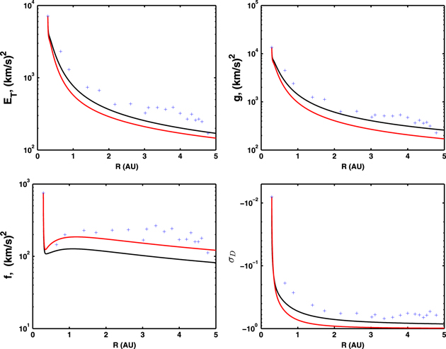
Figure 1. Comparison of the theoretical model with observations from 0.29 to 5 AU. The top-left, top-right, bottom-left, and bottom-right plots describe the theoretical and observed total turbulent energy, the energy in forward propagating modes, the energy in backward propagating modes, and the residual energy, respectively. The solid black and red curves represent the theoretical result with and without including the Alfvén velocity, respectively. The scattered blue plus symbols represent the corresponding observed values.
Download figure:
Standard image High-resolution imageThe residual energy, spontaneously created by turbulent dynamics, is the difference between the fluctuating kinetic and magnetic energy, and is of interest. The numerical solution of the residual energy in normalized form  with and without the Alfvén velocity and their comparison with observation is shown in Figure 1 (bottom right). In the case of equipartition between fluctuating kinetic and magnetic energies, ED, is zero. Close to the Sun, the turbulence is Alfvénic and the kinetic and magnetic fluctuating energies are almost the same, and the observed value of ED at 0.29 AU is close to zero (Figure 1 (bottom right)). Both the theoretical model and the observed residual energy
  increase in a negative sense (
 can be positive or negative) from a value just less than 0 to values approaching −1. Both the observations and the numerical model appear to flatten or plateau between 3 and 5 AU. The evolution of
  with increasing heliocentric distance indicates that
  evolves from an Alfvénic state to one dominated by the energy in magnetic fluctuations. Similarly, the solution that includes the Alfvén velocity (black curve) is closer to observations than that without (red curve). The reason is that the divergence of the background radial IMF acts as source for the residual energy when dominated by the outwardly propagating modes. The normalized residual energy in the absence of a background magnetic field is close to −1 approximately between 3–5 AU, which indicates that the MHD fluctuations are dominated by the magnetic energy. The subsequent evolution beyond 5 AU is described separately below.
Numerical solutions for the three correlation lengths with and without the Alfvén velocity, and their comparison with observations from 0.29 to 5 AU are shown in Figure 2. Figure 2 illustrates the correlation lengths for each of forward and backward propagating modes, and the residual energy. The correlation length is important in MHD turbulence as it controls the dissipation rate of MHD fluctuations. We find that the correlation length  of backward propagating modes f is larger than
  of forward propagating modes g. The reason is that forward propagating modes have initially larger energy than backward propagating modes, and hence the dissipation is initially stronger. Since our energy-containing model is based on a Kolmogorov phenomenology, the correlation lengths will evolve in response to both the decay of turbulence and to the driving of turbulence. Also, the result shows that the correlation lengths
  and
and  (solid and dashed red curves) without the Alfvén velocity lie closer to each other with increasing heliocentric distance than with the Alfvén velocity (solid and dashed black curves). However, the correlation lengths
  (dashed–dotted–dashed black and red curves) with the Alfvén velocity and without are almost the same in both cases. Both
  curves decrease initially and then increase monotonically to 5 AU. The correlation length
  , both with and without VA, is in surprisingly good agreement with the corresponding observed correlation lengths from 0.3–5 AU. Similarly, the correlation length
  exhibits the same increasing trend (and slope) as the observed
  , and is only about a factor of 2 different over the same range. We regard this as satisfactory agreement between the theoretical models and observations. For both
  and
and  , there are few substantive differences between a model with and without VA. The model differences stem from the gradient of the Alfvén velocity, which acts as source for
  and sink for
  . The theoretical correlation length of the residual energy
  shows a larger deviation from the observations (although there is virtually no differences between a model with and without VA). This difference in theory and observations of
  may reflect the uncertainty in the correct form of the model describing the dissipation of residual energy (see the discussion in Zank et al. 2012a and Dosch et al. 2013). The approximate equalization of
  and
and  is discussed further in the following section for the outer heliosphere.

Figure 2. Comparison of the theoretical correlation lengths with observations from 0.29 to 5 AU. The solid, dashed, and dashed–dotted–dashed curves are the theoretical results. The scatter diagram shows observations with the plus symbols corresponding to backward propagating modes, the upward triangles to forward propagating modes, and down-facing triangles the residual energy. The black curves include the Alfvén velocity and the red curves do not.
Download figure:
Standard image High-resolution imageThe numerical solution of the normalized cross helicity  with and without the Alfvén velocity as a function of radial distance, and the corresponding observation are shown in Figure 3 (left). The black and red curves represent the cross helicity with and without the Alfvén velocity, respectively, and both
  curves decrease at different rates with increasing heliocentric distance and both curves bound the observed
  . Also, it is seen that the
  curve is closer to the Helios data and the
  curve to the Ulysses data. This may indicate a basic difference between fast wind in the ecliptic and fast polar wind (including our simplification of using a radial IMF), but this kind of observational study is beyond the scope of this manuscript. The decrease in
  indicates a weakening of the correlation between
  and
and  , which also signifies that forward and backward propagating modes are approximately equally present. The cross helicity can also depend on latitude. There is a noticeable difference in the evolution of the cross helicity when
  is either included or excluded. We believe that the background magnetic field plays a crucial role for generating backward propagating modes. More backward propagating modes are created when the background magnetic field is neglected. Since the cross helicity is simply the difference between the energy in forward and backward propagating modes, the cross helicity in this case goes to zero quickly, and hence decreases faster. The variations in the cross helicity due to the presence or absence of magnetic field may explain the greater scatter in the observations.

Figure 3. Left: comparison of the normalized cross helicity with observations from 0.29 to 5 AU. Right: comparison of the Alfvén ratio with observations from 0.29 to 5 AU. The black curve includes the Alfvén velocity, and the red curve excludes the Alfvén velocity. The scatter plots show the corresponding observed values.
Download figure:
Standard image High-resolution imageFigure 3 (right) compares the theoretically computed Alfvén ratio rA with observations as a function of heliocentric distance from 0.29 to 5 AU. The black and red curve represent the rA with and without the magnetic field, respectively. The rA is the ratio between the fluctuating kinetic and magnetic energy, and is 1 when the fluctuating kinetic and magnetic energy are equal. It starts initially with a value close to 1. At first, both Alfvén ratios decrease from 0.29 AU to around 2 AU, and beyond 2 AU they begin to plateau, the black curve having a value between 0 and 0.2 and the red curve a value between 0 and 0.1. Similarly, the observed rA decreases from 0.29 to ∼2 AU, and then appears to be quite constant up to 5 AU. Although neither solution fully explains the observed rA behavior, the solution with the Alfvén velocity is closer to observations. This, as discussed above, shows that in the inner heliosphere solar wind, turbulence driven by stream shear only tends to become dominated by the energy in magnetic fluctuations i.e., the turbulence is no longer Alfvénic. This behavior is stronger in the absence of the magnetic field than when the field is included. We again caution the reader that comparisons to observations in the inner heliosphere with the current data set have to be interpreted carefully since we use ecliptic Helios data within 1 AU and Ulysses non-ecliptic data from ∼1.5 to ∼5 AU and a radial IMF approximation.
The left and right plots of Figure 4 illustrate the fluctuating magnetic energy density Eb and the solar wind temperature T with and without the Alfvén velocity, respectively and their comparison with observations. The black and red curves are the solutions of Eb and T with and without the Alfvén velocity, respectively and the scattered plus symbols are corresponding observed values. The stream shear source of turbulence drives turbulence in the inner heliosphere, which makes the decay of fluctuations slower than when a turbulence source is absent (Zank et al. 1996; Adhikari et al. 2014). The decay of the fluctuating energy on the other hand is directly proportional to the solar wind temperature. Thus, the solar wind temperature is observed to be higher than expected from adiabatic cooling in the inner heliosphere. The results of Eb and T with  are larger than without
  . This is because the gradient of the Alfvén velocity acts as source for Eb, which slows the decay of Eb. The same reason explains the higher temperature profile when the Alfvén velocity is included. Both results for Eb and T with and without
  are larger than the corresponding observed values. The large scatter in the observed Eb is due to the variability in ρ (mean and fluctuating). Also, T, being a higher order moment, tends to have a large scatter.

Figure 4. Left: comparison of the fluctuating magnetic energy density between the theoretical model and observations. Right: comparison of the solar wind temperature derived from the theoretical model and observations. The black curve includes the Alfvén velocity and the red curve does not. The scatter plus symbols are the observed values corresponding to the Voyager 2 1 hr data.
Download figure:
Standard image High-resolution image6.2. Comparison to Voyager 2 Observations
As previously discussed above, the Alfvén velocity is neglected in this case and the coupled turbulence transport Equations (2)–(8) are solved from 0.29 to 100 AU. Pickup ions are the main source of turbulence beyond the ionization cavity in the outer heliosphere. Thus, the pickup ion source is included in the turbulence transport equations along with the stream–shear source of turbulence. We also compare the theoretical and observational results.
Top left panel of Figure 5 shows the comparison between the theoretical ET and observed ET as a function of heliocentric distance. The red curve indicates the theoretical ET. The green, red, and blue plus symbols indicate the observed R, T, and N components of ET, such as ETR, ETT, and ETN, respectively. The black triangles denote the observed total turbulent energy ET. The comparison between the theoretical g and observed g with increasing heliocentric distance is shown in top right panel of Figure 5. In the figure, red curve describes the theoretical g. The green, red, and blue plus symbols denote the R, T, and N components of g such as gR, gT, and gN, respectively. The black triangles denote the observed total energy of forward propagating modes. The bottom left panel of Figure 5 shows the comparison between the theoretical f and observed f as a function of heliocentric distance. The red curve denotes the theoretical f. The green, red, and blue plus symbols describe the observed R, T, and N components of f such as fR, fT, and fN, respectively. The black triangles denote the total observed energy of backward propagating modes. Figure 5 shows large scatter in the observed R, T, and N components of ET, g, and f, however, the radial dependence of these observed quantities are similar. The total observed energies ET, g, and f also follow similar pattern to that of their components, but are large. It is due to adding up all the components of energy. Interestingly, the comparisons show that the theoretical and observations of ET, g, and f have similar trends with heliocentric distance such as both results decrease monotonically from 1 to 10 AU, and flatten beyond 10 AU. Beyond 10 AU, pickup ions drive turbulence in the outer heliosphere, and hence are thought to be responsible for the flattening of ET, g, and f.
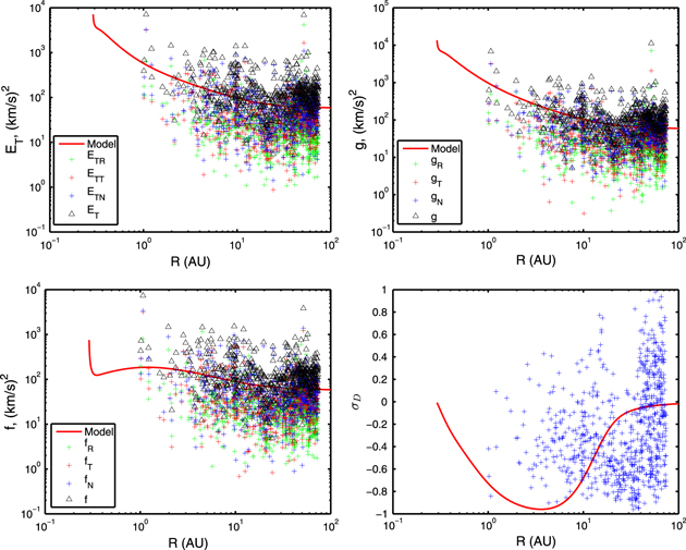
Figure 5. From top left in clockwise order, the plots show respectively the comparison of the theoretical model and the observed total turbulent energy, the energy in forward propagating modes, the normalized residual energy, and the energy in backward propagating modes from 0.29 to 100 AU. The suffix R, T, and N represent R-component, T-component, and N-component of ET, g, and f. The red curves denote the theoretical results and scatter diagrams represent observed values.
Download figure:
Standard image High-resolution imageAn interesting result is the theoretical behavior that is exhibited by the normalized residual energy  beyond 10 AU (Figure 5 (bottom-right)).
  increases toward zero with increasing heliocentric distance. The increasing of
  toward zero means that the kinetic and magnetic energies begin to balance in the outer heliosphere. This result provides an overview of the nature and distribution of the energy in MHD fluctuations throughout the heliosphere. Close to the Sun, there is approximate equipartition between the fluctuating kinetic and magnetic energy. The magnetic energy begins to dominate the MHD fluctuations within about 10 AU. After that, the kinetic energy gradually becomes larger, and eventually the magnetic and kinetic energy are approximately equipartitioned. Observations show a large scatter in the observed value of
  , which makes detailed comparison difficult. The scatter may be due to variations in the fluctuating kinetic energy and solar wind density.
Figure 6 illustrates the comparison of radial evolution of the theoretical and observational correlation lengths  and
and  of forward and backward propagating modes, respectively, and the correlation length
  of the residual energy ED from 0.29 to 100 AU. The blue curve and blue circles identify theoretical and observed
  , respectively, the red curve and red triangles the theoretical and observed
  , and the green curve and green diamonds the theoretical and observed
  . By comparing with previous results (Figure 2), the correlation lengths
  and
and  beyond 5 AU continue to approach one another, and beyond 10 AU they are approximately equal. With increasing heliocentric distance, the two correlation lengths
  and
and  converge indicating that forward and backward propagating modes are tending toward approximately equal energies, and vice versa i.e.,
  (Matthaeus et al. 1996), and both energy modes probably follow the same energy spectrum i.e., both have the same decay rate.
  increases gradually to 10 AU, and then beyond 10 AU increases more rapidly. The comparison shows that the theoretical and observational
  and
and  agree reasonably well, as does
  up to ∼10 AU. Beyond 10 AU, the theoretical
  increases because the pickup ions do not effect on the residual energy (Equation (21)), and hence on
  . The other reason for the discrepancy may be the uncertainty in the correct form of the dissipation term in the evolution of the residual energy. This requires further theoretical investigations.
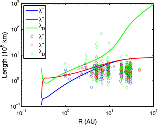
Figure 6. Comparison of the theoretical and observed correlation lengths as a function of heliocentric distance. The blue, red, and green curves correspond to the theoretical correlation lengths of forward propagating modes, backward propagating modes, and the residual energy, respectively. The blue, red, and green scatter diagrams correspond to the corresponding observed correlation lengths.
Download figure:
Standard image High-resolution imageThe left and right plots of Figure 7 compare the theoretical curve and observations of the normalized cross helicity  and the Alfvén ratio rA as a function of heliocentric distance from 0.29 to 100 AU, respectively. Again, like the previous results,
  continue to decrease monotonically beyond 5 AU, and approaches zero beyond ∼30 AU. The tendency for
  to be approximate zero beyond ∼30 AU is consistent with the findings of Breech et al. (2005), although Breech et al. (2005) also considered the latitude dependence of the cross helicity. However, we have the further interesting result that the Alfvén ratio rA changes profoundly beyond 10 AU and gradually increases to ∼1 beyond ∼30 AU. As before, the result suggests that the magnetic energy dominates in MHD fluctuations within ≲10 AU and then the kinetic energy begins to increase beyond ≳10 AU. It also signifies that close to the Sun and in the outer heliosphere beyond ∼30 AU, the kinetic and magnetic energies are approximately equipartitioned, which also means that the fluctuations are Alfvénic. In the case of outer heliosphere, this in large part is due to the injection of Alfvénic turbulence by pickup ions—see Equation (21).

Figure 7. Left: comparison between the theoretical and observations of the normalized cross helicity as a function of heliocentric distance from 0.29 to 100 AU. Right: comparison between the theoretical and observations of the Alfvén ratio as a function of heliocentric distance from 0.29 to 100 AU.
Download figure:
Standard image High-resolution imageThe left and right plots of Figure 8 describe the fluctuating magnetic energy density Eb, and the solar wind temperature T, and their comparison with observations as a function of heliocentric distance from 0.29 to 100 AU, respectively. The stream-shear source of turbulence is assumed to be important within 4–5 AU, and the pickup ion source of turbulence is important beyond the ionization cavity. These sources drive turbulence throughout the heliosphere, and make the decay of f, g, and ED slower. Since Eb depends on these quantities (Equation (11)), the slower decay of f, g, and ED causes the slower decay of Eb as well. Importantly, the decay of these parameters is directly proportional to the solar wind temperature, so the observed temperature is higher than is expected for adiabatic cooling. Due to the presence of pickup ions in the outer heliosphere, the profiles of f and g become a little flattened. Thus, the flattening of Eb and the increase of T beyond 20 AU can be considered due to the presence of pickup ions in the outer heliosphere. In the left figure, the  , EbT, and EbN correspond to the observed R, T, and N components of Eb, which are shown by red, green, and blue plus symbols, respectively. The black triangles indicate the total observed Eb. All the observed results EbR, EbT, EbN, and Eb show large scatter, which may be due to the variation in the solar wind density. In the absence of the solar wind density, the observed value is less scattered (see Figure 9 (left)). The comparisons of the theoretical and observed, Eb and T, show that the theoretical results well reproduce the observations.
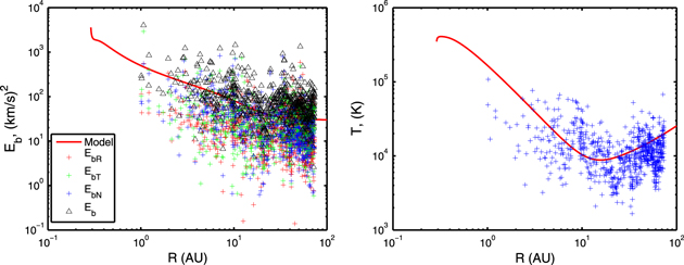
Figure 8. Left: comparison of the fluctuating magnetic energy density between the theoretical model and observations from 0.29 to 100 AU. Right: comparison of the solar wind temperature between the theoretical model and observations from 0.29 to 100 AU. The scatter diagrams show the observed values derived from Voyager 2 1 hr data. The suffix R, T, and N represent R-component, T-component, and N-component of Eb.
Download figure:
Standard image High-resolution image
Figure 9. Left: comparison between the theoretical and observations of fluctuating magnetic energy as a function of heliocentric distance. Right: comparison between the theoretical and observations of fluctuating kinetic energy as a function of heliocentric distance. The solid curves are theoretical results, and the scattered diagrams are observed values. The suffix R, T, and N represent R-component, T-component, and N-component of the fluctuating magnetic and kinetic energies, respectively.
Download figure:
Standard image High-resolution imageThe left plot of Figure 9 shows the fluctuating magnetic energy b2 as a function of heliocentric distance. We use Equation (11) to calculate b2. The comparison shows a good agreement between the theoretical and observational results with heliocentric distance. This result is similar to that of Zank et al. (1996), but based on their very simplified model. The right plot of Figure 9 describes the fluctuating kinetic energy u2 as a function of heliocentric distance. Equation (6) i.e.,  of Zank et al. (2012a) is used to calculate u2. The observations show a large scatter in u2, which may be due to greater variability in the plasma data. The comparison between the theoretical and observational results shows that the theoretical result is consistent with observations beyond 5 AU. Our results may well improve if we refine the form of dissipation term in the residual energy transport equation. We also compare the theoretical results with the Voyager 2 observations based on outwardly directed magnetic field only, in Appendix
7. DISCUSSION AND CONCLUSION
The Zank et al. (2012a) model that describes the transport of MHD turbulence in inhomogeneous flows addresses many of the limitations of earlier models by Matthaeus et al. (1994, 2004), Zank et al. (1996), and Breech et al. (2005, 2008; see Table 2).
Table 2. Limitations of Previous Models
| Models | Ranges | Limitations |
|---|---|---|
| Matthaeus et al. (1994) | 0.05–2 AU | Neglects Alfvén velocity, and sources of turbulence. |
| Zank et al. (1996) | 1–100 AU | Neglects Alfvén velocity, assumes zero cross helicity, and does not consider the residual energy, energies corresponding to forward and backward propagating modes, and the respective correlation lengths. |
| Matthaeus et al. (2004), Breech et al. (2005), and Breech et al. (2008) | 0.3–100 AU | Neglects Alfvén velocity in the inner heliosphere, does not consider the residual energy, energies corresponding to forward and backward propagating modes, and the respective correlation lengths. |
Download table as: ASCIITypeset image
Here we used two models and two data sets to study the transport of MHD turbulence from 0.29 to 5 AU, and from 0.29 and 100 AU. In the region from 0.29 to 5 AU, we solved the 1D steady state form of the coupled turbulent transport equations in spherical coordinates with and without the Alfvén velocity, and we neglect  in the region from 0.29 to 100 AU. In both cases, the theoretical results were compared with the corresponding observed values, taken from Helios 2, Ulysses, and Voyager 2 data sets. The seven coupled turbulence transport equations used in this paper provides a complete description for the transport of MHD turbulence moments throughout the solar wind. Similarly, the numerical solutions presented in this paper are the first detailed solutions of the Zank et al. (2012a) model throughout the heliosphere.
Unlike previous models, we include the residual energy and the various correlation lengths, all of which allow for a more detailed description (and comparison) of the turbulent state of the heliosphere. We used ecliptic Helios 2 data within 1 AU and non-ecliptic  data from ∼1.5 to ∼5 AU. For this data set, we examined the effect of a non-zero
  , with the approximated IMF as radial. The numerical solutions with and without the Alfvén velocity show that the inclusion of
  modifies the turbulence transport model, but the trend of the solutions in both cases is similar. Comparison of the model with observations validates the theory reasonably well. Despite the complications in approximating the IMF as radial for the combined Helios 2 and
  data sets, some general conclusions are that the turbulence transport model of Zank et al. (2012a; with and without
  ) accounts for
- (1)the decay of the total turbulent energy ET;
- (2)the decay of the outwardly propagating modes g;
- (3)the generation by shear driving and subsequent decay of inwardly propagating modes f;
- (4)the decay of the residual energy ED (or
 ), and
 - (5)the increase in the correlation lengths, and with increasing heliocentric distance.


The radial evolution of the solutions with and without  bracketed the observed decay of the normalized cross helicity. Note that our solutions for the normalized residual energy
  and the Alfvén ratio rA show that the equipartition between kinetic and magnetic energy decreases with increasing heliocentric distance, implying that MHD fluctuations are eventually dominated by the magnetic energy. The fluctuations are more magnetically dominated when the Alfvén velocity is neglected than included. Finally, we also find that the correlation lengths corresponding to backward and forward propagating modes,
  and
and  , respectively, converge to a single value more rapidly within 5 AU when the Alfvén velocity is neglected. In contrast, results of
  do not change with and without the Alfvén velocity.
In the region from 0.29 to 100 AU, our results for the generation and transport of turbulence clarify and/or predict a better understanding of the distribution of turbulence throughout the heliosphere. The results are summarized as follows.
(1) We find that all the energies decrease monotonically beyond 5 AU.
(2) We find that the normalized residual energy  and the Alfvén ratio rA gradually increase after ∼10 AU, reversing the trend from the inner heliosphere, and tending to ∼1 after ∼30 AU. We predict that turbulence in the inner heliosphere evolves toward a magnetically dominated state until about 10 AU, after which it tends toward a state where kinetic and magnetic energies are equipartitioned. This is largely due to the generation of turbulence by PUIs in the outer heliosphere.
(3) We also find that our results for the normalized cross helicity  , and the correlation lengths
  and
and  are consistent with a phenomenology of
  as in Matthaeus et al. (1996). Beyond 30 AU,
  and
and  are approximately equal and
  is almost equal to zero, which means that forward and backward propagating modes are equally present.
(4) The theoretical fluctuating magnetic energy density Eb, the solar wind temperature T, and the fluctuations in the magnetic field b2 are in a good agreement with observations.
Finally, the comparisons between the theoretical and observations show that our theoretical results reproduce similar trends to that of the observations. Thus, we conclude that the theory of Zank et al. (2012a) can describe the transport of turbulence in the super-Alfvénic solar wind.
We acknowledge the partial support of NASA grants NNX14AC08G and NNX11AO64G. R.B. and D.T. were supported by the Agenzia Spaziale Italiana under contract ASI/INAF I/013/12/0. Helios 2 plasma data were kindly provided by H. Rosenbauer and R. Schwenn (MPAE, Katlenburg-Lindau). Magnetic field data are from the Rome-University /CNR-IFSI/NASA-GSFC magnetometer (PIs F. Mariani and N. F. Ness). Data from ULYSSES were obtained from NASA-CDAWeb.
APPENDIX A: OUTWARDLY DIRECTED MAGNETIC FIELD
As discussed earlier (Section 5), the results of Appendix A correspond to outwardly directed magnetic field only. Our reason for doing this is that we consider outwardly directed magnetic field in our theoretical work. In this regard, a better comparison between theory and observations is made. The observational results now contain fewer data points than the previous results of Section 6.2. However, the trend of both sets of observations is similar. Figure 10 (top-left) compares the theoretical and observed ET; Figure 10 (top-right) compares the theoretical and observed g; and Figure 10 (bottom-left) compares the theoretical and observed f. Both theoretical and observational results decrease with increasing heliocentric distance in a similar fashion. Figure 10 (bottom-right) compares the theoretical and observed normalized residual energy. Again, there is a large scatter in the observed normalized residual energy  .
.
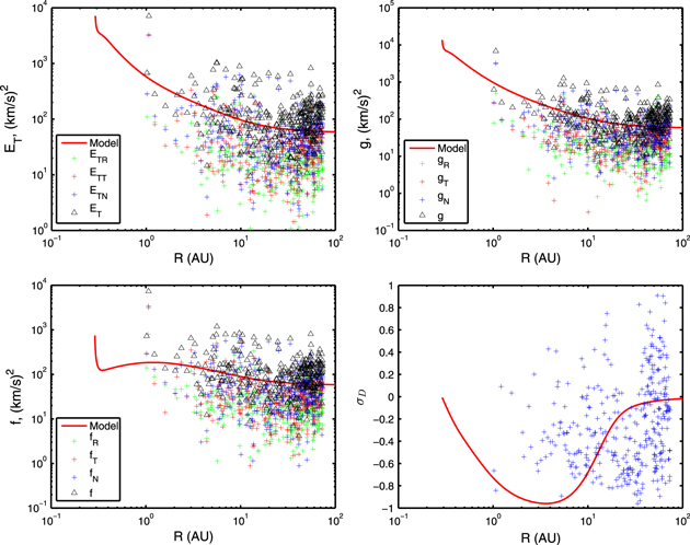
Figure 10. From top left in clockwise order, the plots show respectively the comparison of the theoretical model and the observed total turbulent energy, the energy in forward propagating modes, the normalized residual energy, and the energy in backward propagating modes from 0.29 to 100 AU, respectively. The solid curves are theoretical results and the scatter diagrams are observed values. The suffix R, T, and N represent R-component, T-component, and N-component of ET, g, and f, respectively.
Download figure:
Standard image High-resolution imageThe left and right plots of Figure 11 compares the theoretical and observed normalized cross helicity  and the Alfvén ratio rA, respectively. There is large scatter in the observed values of both
  and rA. The theoretical Alfvén ratio does not reproduce the observed rA within 10 AU, but beyond 10 AU is consistent. The theoretical and observed
  agree reasonably well.

Figure 11. Left: comparison between the theoretical and observed normalized cross helicity as a function of heliocentric distance from 0.29 to 100 AU. Right: comparison between the theoretical and observations of the Alfvén ratio as a function of heliocentric distance from 0.29 to 100 AU.
Download figure:
Standard image High-resolution imageThe left and right plots of Figure 12 compares the theoretical and observed fluctuating magnetic energy density Eb, and solar wind temperature T as a function of heliocentric distance, respectively. Both comparisons show that the trends of theory and observation are similar. In the figure, R, T, and N describe the R-component, T-component, and N-component of the fluctuating magnetic energy density.

Figure 12. Left: comparison of the fluctuating magnetic energy density between the theoretical model and observations from 0.29 to 100 AU. Right: comparison of the solar wind temperature between the theoretical model and observations from 0.29 to 100 AU. The solid red curves represent the theoretical results. The scatter diagrams show the observed values derived from Voyager 2 1 hr data. The suffix R, T, and N represent R-component, T-component, and N-component of Eb.
Download figure:
Standard image High-resolution imageThe comparison of the theoretical and observational fluctuating magnetic energy b2 and fluctuating kinetic energy u2 are shown in the left and right panels of Figure 13, respectively. Here, the comparison of b2 shows good agreement between theory and observations. Although, the theoretical u2 is inconsistent with observations within 5 AU, it is consistent beyond 5 AU.

Figure 13. Left: comparison of the fluctuating magnetic energy between the theoretical model and observations from 0.29 to 100 AU. Right: comparison of the fluctuating kinetic energy from 0.29 to 100 AU. The scatter diagrams show the observed values derived from Voyager 2 1 hr data.
Download figure:
Standard image High-resolution imageAPPENDIX B: SOLAR WIND PARAMETERS
Here we show results that correspond to both an inwardly and outwardly directed magnetic field. The top left plot of Figure 14 shows the R, T, and N components of the solar wind velocity, UR, UT, and UN, respectively, as a function of heliocentric distance. The solid horizontal line shows an average UR (∼444 km s−1). UR varies between a maximum speed ∼520 km s−1 and minimum speed ∼350 km s−1, and follows the solar cycle. The T and N components of the solar wind speed are smaller than UR. The observed results show that UT and UN are approximately similar within 40 AU, but UT is mostly positive beyond 40 AU, and UN is negative beyond 40 AU.

Figure 14. Top-left: solar wind velocity as a function of heliocentric distance. Top-right: magnetic field as a function of heliocentric distance. Bottom: solar wind density as a function of heliocentric distance. The red curve describes  , where
  is the solar wind density at r0 (=0.29 AU).
Download figure:
Standard image High-resolution imageThe top right plot of Figure 14 shows the R, T, and N components of the magnetic field, BR, BT, and BN, respectively, as a function of heliocentric distance. The observed BR shows that it has both positive and negative values. Here, positive BR indicates outward magnetic field with respect to the Sun, and negative BR indicates inward field. The results presented in Section 6.2 correspond to both outward and inward magnetic field. BT and BN also have both positive and negative values with increasing heliocentric distance.
The bottom plot of Figure 14 illustrates the solar wind density as a function of heliocentric distance. The red curve shows  , where
  is the solar wind density at r0 = 0.29 AU. To find the density at 0.29 AU, we use an empirical density relation (Equation (30) of Chandran & Hollweg 2009), which gives approximately 56 cm−3. The comparison shows that the observed density follows
  , with a slight deviation beyond ∼50 AU.
APPENDIX C: SOLAR WIND PARAMETERS: OUTWARD MAGNETIC FIELD ONLY
The results in this section and in Appendix A correspond to outwardly magnetic field only, as illustrated by BR in the magnetic field plot of Figure 15 (top-right). The Figure 15 (top-right) shows that all the BR are positive, whereas BT and BN show both positive and negative values with increasing heliocentric distance. Figure 15 (top-left) shows UR, UT, and UN as a function of heliocentric distance. The solid horizontal line represents an average UR (=445 km s−1). Similarly, the bottom plot describes the solar wind density as a function of heliocentric distance, where the red curve describes  . The results of Appendix C are similar to Appendix B.

Figure 15. Top-left: solar wind velocity as a function of heliocentric distance. Top-right: magnetic field as a function of heliocentric distance. Bottom: solar wind density as a function of heliocentric distance. The red curve describes  , where
  is the solar wind density at r0 (=0.29 AU).
Download figure:
Standard image High-resolution image