


ABSTRACT
The circular ribbon of enhanced energetic neutral atom (ENA) emission observed by the Interstellar Boundary Explorer (IBEX) mission remains a critical signature for understanding the interaction between the heliosphere and the interstellar medium. We study the symmetry of the ribbon flux and find strong, spectrally dependent reflection symmetry throughout the energy range 0.7–4.3 keV. The distribution of ENA flux around the ribbon is predominantly unimodal at 0.7 and 1.1 keV, distinctly bimodal at 2.7 and 4.3 keV, and a mixture of both at 1.7 keV. The bimodal flux distribution consists of partially opposing bilateral flux lobes, located at highest and lowest heliographic latitude extents of the ribbon. The vector between the ribbon center and heliospheric nose (which defines the so-called BV plane) appears to play an organizing role in the spectral dependence of the symmetry axis locations as well as asymmetric contributions to the ribbon flux. The symmetry planes at 2.7 and 4.3 keV, derived by projecting the symmetry axes to a great circle in the sky, are equivalent to tilting the heliographic equatorial plane to the ribbon center, suggesting a global heliospheric ordering. The presence and energy dependence of symmetric unilateral and bilateral flux distributions suggest strong spectral filtration from processes encountered by an ion along its journey from the source plasma to its eventual detection at IBEX.
Export citation and abstract BibTeX RIS
1. INTRODUCTION
The Sun, with its radially outflowing solar wind plasma, moves through the interstellar medium along an ecliptic vector direction  Sun(λ, β) = (259°, 5°) that is derived from inflow measurements of the neutral component of the ISM plasma (McComas et al. 2012a; Bzowski et al. 2012; Möbius et al. 2012). This motion, which lies near the heliographic equator, creates the heliospheric cavity in the interstellar medium, and
  Sun is an important ordering parameter for the global structure and dynamics of the interaction between the solar wind and ISM. A simplistic hydrodynamic picture of the interaction of these plasmas results in a bullet-shaped heliosheath with cylindrical symmetry around
  Sun (Parker 1961).
Numerous processes can introduce asymmetries to this global structure (e.g., Zank 1999), and many of these processes have strong internal order and spatial or temporal symmetry. For example, the properties of the solar wind, which is a dominant energy and mass input in the heliosheath, has cylindrical symmetry around the heliographic poles as well as reflection symmetry near the heliographic equator that results from fast solar wind at high latitudes and slower, denser solar wind at low latitudes. As another example, the presence of an interstellar magnetic field  can strongly influence the Sun–ISM interaction, depending on its magnitude and direction (e.g., Fahr et al. 1988; Zank 1999; Zank et al. 2009). Finally, temporal symmetries can be introduced by the cyclical variation of the solar wind structure and the Sun's magnetic field vector over the solar cycle. On a global scale, observational signatures of these symmetries can provide insight into the predominant dynamic processes that govern the Sun–ISM interaction.
The unexpected but dominant feature in the first sky map of energetic neutral atoms (ENAs) measured from Interstellar Boundary Explorer (IBEX; McComas et al. 2009a) is the so-called ribbon of enhanced ENA flux (McComas et al. 2009b). The ribbon is narrow (∼20°) in width (Fuselier et al. 2009; Schwadron et al. 2011) and circular with the center near ecliptic coordinate (λ, β) = (221°, 39°) (Funsten et al. 2009a). Recent analysis (Funsten et al. 2013) using 3 yr of IBEX data has refined the ribbon center to (λ, β) = (219 2 ± 13, 399 ± 23) and quantified the energy dependence of the ribbon center; additionally, the ribbon was found to have strong circularity, spanning a half cone angle of 745 ± 20 in the sky and whose precision is less than the intrinsic 65 imaging resolution of the IBEX-Hi ENA imager (Funsten et al. 2009b). The circularity of the ribbon is evidence of strong cylindrical symmetry, with the ribbon center as the cylindrical symmetry axis that defines a fundamental direction that governs the overall structure responsible for the ribbon ENA emission.
The ribbon center is generally consistent with the average ISM magnetic field direction along lines-of-sight to nearby stars (e.g., Frisch et al. 2010, 2012), and current interpretation of the ribbon places the pristine interstellar magnetic field direction  along the vector from the Sun to the ribbon center, with enhanced ENA emission observed when the radial line-of-sight vector from the inner heliosphere is perpendicular to
  , i.e.,
  for which
  is the perturbed ISM magnetic field in the vicinity of the heliosphere (e.g., Schwadron et al. 2009). Of particular interest in this study are symmetries associated with the circular ENA emission of the ribbon, which is apparently centered at and therefore ordered by
  . 3D MHD modeling of the Sun–ISM interaction (Pogorelov et al. 2008a; Zank et al. 2009), as well as simulations of the interaction of ISM dust in the heliosphere (Slavin et al. 2010), have identified as an important ordering parameter the so-called BV plane, which contains the Sun and the vector between
  and
and  Sun. Assuming the ribbon center corresponds to
  , the BV plane in the IBEX sky maps is defined by the vector between the ribbon center and the heliospheric nose.
The ENA spectral distribution can be generally characterized as a power law (McComas et al. 2009b; Livadiotis et al. 2011; Dayeh et al. 2011; Desai et al. 2012, 2014; Fuselier et al. 2014), and the ENA flux likely reaches a maximum near 100 eV (Fuselier et al. 2014). Variability of spectra over the ENA sky maps indicates the spectra follow the general latitudinal ordering of the solar wind (Funsten et al. 2009a; Dayeh et al. 2012; McComas et al. 2012b; Livadiotis et al. 2013), are influenced by heliospheric pickup ion populations (Livadiotis et al. 2012), and may be composed of multiple source ion populations (Desai et al. 2014). Temporal variation is also consistently observed in the sky maps, with a general reduction in ENA flux over time (McComas et al. 2010) that appears to be driven by reduction in the solar wind over the current solar cycle (McComas et al. 2012b; Kucharek et al. 2013). An energy-dependent temporal variation and a north–south temporal asymmetry of ENA flux is systematically observed at the ecliptic poles (Reisenfeld et al. 2012; Allegrini et al. 2012), which are viewed continuously throughout the IBEX mission and thus serve as a statistically robust temporal baseline.
The ribbon is an exquisitely sharp and systematic feature in the ENA sky maps and thus is an important signature for understanding the structure and properties of the source plasma that is believed to be heliospheric in origin. A hot plasma (such as in the heliosheath) immersed in a cold neutral background (such as the ISM neutral atoms that permeate the heliosheath) will emit ENAs whose spectral distribution and flux retain specific information about the properties of the source plasma. Here, we define "filtration" as the spectral, spatial, and temporal processes that act on this ENA emission and alter its properties, thus obscuring the embedded information of the source plasma properties.
A plethora of hypotheses have been posed to explain the ribbon. Most start with initial ENA emission from a source plasma in the heliosphere and subsequently follow different spatial, spectral, and temporal filtration processes that occur between initial ENA emission and their observation at IBEX (see the recent summary of McComas et al. 2014b). Several hypotheses of so-called secondary ENA emission (McComas et al. 2009b; Chalov et al. 2010; Heerikhuisen et al. 2010; Schwadron & McComas 2013; Möbius et al. 2013) explain the ribbon structure as resulting from ENAs that are initially emitted from a source plasma inside the heliosphere (solar wind and inner heliosheath) and propagate into the ISM, are ionized and captured on ISM magnetic field lines, and are eventually neutralized again as "secondary" ENAs that can travel into the inner heliosphere, where they can be detected by IBEX.
Modeling of these secondary ENA processes in the ISM–heliospheric interaction via magneto-hydrodynamic (MHD) simulations (e.g., Heerikhuisen et al. 2011; Pogorelov et al. 2011) and analytic calculations (Schwadron & McComas 2013) are consistent with a spatial filtering process in which (1) the ribbon center is the likely direction of  , (2) the arc traced by the ribbon is the result of perturbation of the interstellar magnetic field geometry by the heliosphere, and (3) enhanced emission of secondary ENAs occurs from viewing locations in which the line-of-sight
  from the inner heliosphere is perpendicular to the perturbed ISMF vector, i.e.
  . These processes that induce spatial filtration are also energy-dependent and thus introduce spectral filtration.
For this "secondary" hypothesis, filtration processes are complex and include the energy-dependent radial distance that an initial ENA travels into the ISM before it is ionized; the  retention dynamics of the ionized primary ENAs that are spatially, spectrally and temporally dependent and depend on
  and its perturbation in the vicinity of the heliosphere; the contributions from multiple heliospheric plasma sources to a "retained" ion population at a specific location along
  in the ISM; and ionization losses of secondary ENAs as they travel to the inner heliosphere. Under any hypothesis for the ribbon, understanding and quantifying these filtration processes and their influence on the observed ENA distributions is essential for extracting source plasma properties from ENA images.
Because of this complexity, parameterizing the global properties of the ribbon using compact representations, such as ribbon circularity and its center location in the sky, are crucial for testing these hypotheses and understanding the global structure, dynamics, and origin of the ribbon. The presence of symmetry and identification of symmetry axes likewise provide powerful insight into the global ENA emission of the ribbon. In this study we quantify and analyze the symmetry of ENA flux distributed around the circular ribbon as a function of ENA energy.
Inspection of the ribbon-centered flux maps used for this study (Figure 2 of Funsten et al. 2013) shows qualitatively that the ribbon at lower energy (∼1 keV) appears to consist of a single ENA flux peak broadly distributed around the circular ribbon while at higher energy (2–4 keV) contains two opposing flux peaks. The objective of this study is to quantify the regularity of this symmetry over the entirety of the ribbon, obtain any global ordering parameters arising from its symmetry (such as a symmetry plane), and compare them with other parameters that may govern the ENA emission, such as heliospheric latitude and the direction of motion of the Sun in the ISM. We assume throughout our symmetry analysis that the ribbon center lies within the symmetry plane of any symmetry features discovered within the ribbon.
2. IBEX OBSERVATIONS
Figure 1 shows annular ENA flux maps at 6° × 6° resolution used for this study. They were obtained from the IBEX-Hi neutral atom imager (Funsten et al. 2009b) and span five energy passbands at nominal energies 0.7, 1.1, 1.7, 2.7, and 4.3 keV. The ENA flux maps, fully described in McComas et al. (2014a), cover the first five years of the IBEX mission, include IBEX orbits 11 through 230, and are acquired from IBEX viewing in the ram direction only. The maps are corrected for the Compton–Getting effect (McComas et al. 2012b) and for ENA extinction as calculated along the ENA trajectories through the inner heliosphere to the IBEX spacecraft (McComas et al. 2012b, 2014a; Bzowski 2008).

Figure 1. IBEX ENA flux map F(θ, ϕ) at each of the five energy passbands is rotated into a ribbon-centric reference frame centered at ecliptic (221°, 39°). In this frame the heliospheric nose lies along the azimuth θ = 0° axis; ϕ is the polar (radial) angle from the ribbon center. The white lines are the circular fits to the ribbon flux from Funsten et al. (2013). The red lines show the primary (sagittal) symmetry axes derived from this study. The following directions are noted in each map for reference: EN = Ecliptic North, Nose = heliospheric nose, and V1 and V2 are the locations of the Voyager 1 and 2 spacecraft in the sky.
Download figure:
Standard image High-resolution imageFollowing the frame used for analysis of the ribbon circularity (Funsten et al. 2013), we project the IBEX ENA flux data onto a ribbon-centered spherical coordinate frame (azimuth, polar) = (θ, ϕ) centered on ecliptic (221°, 39°) for all energies. Our objective is to understand systematic symmetry and its spectral variation on a global scale, so we use this single frame even though the ribbon center at 4.3 keV appears slightly offset from the ribbon center at lower energies (Funsten et al. 2013). In this rotated system, the ribbon center lies nearly at (0°, 0°), and the polar (radial) angle ϕ corresponds to the angle between a point in the sky and (0°, 0°). The azimuth angle θ ranges from 0° to 360° around the ribbon center. The heliospheric nose direction, which is defined at ecliptic  Sun(λ, β) = (259°, 5°) (McComas et al. 2012a; Bzowski et al. 2012; Möbius et al. 2012), is located along the θ = 0° axis in the rotated frame. The ribbon flux peak is generally found within the polar angle range 70° < ϕ < 85°, so we use the annular flux maps over the polar angle range 48°–102° (nine polar pixels of 6° width) that fully includes the ribbon as the base data set for this study.
The azimuthal angle θ is defined specifically in reference to the ribbon-centered coordinate system of Figure 1. Within this ribbon-centered frame, we introduce three azimuthal reference angles that are used as input (roll angle θR) and output (angles θS and θT of primary and secondary reflection symmetry) of the symmetry analysis. Because we find that the ribbon has strong bilateral symmetry at high energies, we borrow the term "sagittal" to refer to the primary reflection symmetry axis and "transverse" as a secondary symmetry axis. These reference angles are defined relative to the ribbon center–heliospheric nose vector that lies at θ = 0°, which, assuming the ribbon center location corresponds to the pristine ISM magnetic field vector direction  , corresponds to the BV plane.
Distinct features of the structure of the ribbon simplify investigation of its symmetry. First, the ribbon is narrow in polar angle and highly circular in azimuthal angle as projected on the sky. Standard methods for symmetry identification in an image usually first identify an object's symmetry center; the ribbon-centered reference frame of Figure 1 provides the natural coordinate system for its symmetry, and our analysis defines the symmetry axes as traversing the ribbon center (0°, 0°). Second, the ribbon flux as a function of polar angle ϕ is reasonably represented by a Gaussian distribution (Schwadron et al. 2011, 2014) and more precisely represented as a systematically skewed (asymmetric gamma) distribution, with a wider peak toward the ribbon interior (Funsten et al. 2013). Because this flux peak lies tightly and systematically along the ribbon circle, our analysis focuses on variation of the ribbon flux F(θ) as a function of azimuthal angle only. In summary, the ribbon scribes a circle in our ribbon-centered coordinate system, the ribbon flux peak is narrow in polar angle, and strong flux symmetries are observed as a function of azimuthal angle only.
2.1. Autocorrelation of IBEX Flux Maps: An Indicator of Ribbon Symmetry
The human brain is conditioned to identify symmetry (Enquist & Arak 1994; Rhodes 2006), and inspection of the distribution of ENA flux around the ribbon in the flux maps of Figure 1 indicates a single, broad flux peak at low energies with apparent reflection symmetry and two flux peaks of similar azimuthal width and largely opposing (on opposite sides of the ribbon) at the high energies.
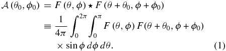
Cross-correlation is routinely used to identify periodic patterns in data and thus can be used as an indicator of the presence of symmetric features in an image (Reichardt 1961; Neubecker 1996; Masuda et al. 1993), thus providing quantitative insight of our visual inspection of Figure 1. We examine rotational symmetry using the autocorrelation  using the annular flux map F(θ, ϕ) at each energy in Figure 1 as a function of 6° increments of azimuthal (θ0) and polar (ϕ0) offset angles:
From Equation (1), we derive the autocorrelation score  , where
  and
and  are the minimum and maximum values of
  of each map. Values of χ = 0 and χ = 1 correspond to the lowest and highest autocorrelation, respectively, in each flux map.
The autocorrelation score is shown in Figure 2 for each of the annular flux maps of Figure 1 as a function of azimuthal and polar offset angles, with red corresponding to higher autocorrelation and blue corresponding to lower autocorrelation. As expected, the maximum value of χ lies at the center of the primary autocorrelation peak, (θ0, ϕ0) = (0°, 0°). As the polar and azimuth offset angles increase from 0°, χ slowly decreases at a rate that indicates the characteristic spatial sizes of the ribbon flux peak(s) in these angular directions.
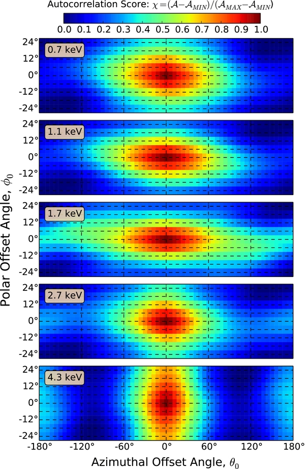
Figure 2. Autocorrelation score χ(θ0, ϕ0) is shown for each of the annular flux maps of Figure 1 as a function of azimuthal (θ0) and polar (ϕ0) offset angles used in Equation (1). Values of χ = 0 and χ = 1 correspond to the lowest and highest autocorrelation, respectively, in each flux map. The autocorrelation maps provide a qualitative indication of the presence of rotational symmetry of the ribbon flux and the possible presence of symmetric flux peaks.
Download figure:
Standard image High-resolution imageIn polar angle, regions of higher χ appear to be narrow (⩽24°) and generally centered at polar offset angle ϕ0 = 0°, confirming that the ribbon flux is narrow in polar angle, highly circular, and well-centered in the ribbon-centered coordinate frame.
In azimuthal angle, only a single autocorrelation peak, centered at θ0 = 0°, is observed at 0.7 and 1.1 keV, suggesting the ribbon flux is unimodal. This autocorrelation peak narrows by ∼30% at 2.7 and ∼50% at 4.3 keV. Additionally, at 2.7 keV and 4.3 keV, a secondary autocorrelation peak centered near θ0 = ±180° is clearly observed, suggesting the presence of two (bilateral) flux lobes that are generally located on opposite sides of the circular ribbon.
2.2. IBEX Data for Reflection Symmetry Analysis
While the autocorrelation analysis clearly reveals the existence of rotational symmetry of the ribbon flux as well as the presence of multiple flux peaks with rotational symmetry, it does not provide a quantitative test for symmetry or the location of symmetry axes. For quantitative symmetry analysis, we test for reflection symmetry using correlation analysis of the annular flux maps of Figure 1. For this study, we do not separate the ribbon flux from the spatially slowly varying globally distributed flux (Schwadron et al. 2011, 2014); thus our results are characteristic of a combined azimuthally varying ribbon flux and a slowly varying globally distributed flux at each energy. We employ several input data sets for the correlation analysis:
- 1.F(θ, ϕ): the 2D annular ENA flux maps of Figure 1, which span nine polar pixels in the angular range 48°–102° that are generally centered on the ribbon.
- 2.FP9(θ): at each azimuthal angle θ, the average ENA flux of all nine polar pixels (which span 48°–102°) and, at most energies, fully contains the ribbon flux. Because FP9(θ) includes the flux of nine pixels at each θ, it is the most statistically significant data. However, it also includes regions inside and outside of the ribbon peak that are largely dominated by the globally distributed flux and is therefore comparatively less sensitive to variations of the ribbon flux over azimuthal angle.
- 3.FP2max(θ): at each azimuthal angle θ, the average flux of the two adjacent polar pixels of maximum flux within the nine polar pixels spanning 48°–102°. This flux is derived from only two pixels and thus provides comparatively poorer statistics; however, because FP2max(θ) includes a comparatively larger fraction of the ribbon flux than FP9(θ), it provides better insight into azimuthal variations of ribbon flux. Note that FP2max(θ) > FP9(θ) for any θ.
3. TESTS OF REFLECTION SYMMETRY
We test the azimuthal dependence of ribbon flux for reflection symmetry, for which perfect reflection symmetry is obtained if the following is true over all angles −180° ⩽ θ ⩽ +180°:

Throughout this paper, we use θ to denote an azimuthal angle measured relative to the ribbon center–heliospheric nose vector, which lies in the BV plane, and Θ to denote an azimuthal angle measured relative to the primary (sagittal) symmetry axis θS. Because an axis of symmetry traverses the ribbon center and bisects the circular ribbon, the axis of symmetry at θS can equivalently be defined at the opposite side (i.e., θS + 180°) of the ribbon. We note that our test for reflection symmetry also clearly identifies rotational symmetry, in which flux peaks may be periodically distributed around the ribbon and for which n-fold symmetry yields n − 1 symmetry axes.
As illustrated in Figure 3 for the 2D flux map F(θ, ϕ) at 4.3 keV, our reflection symmetry test starts with "folding" the flux map along an axis defined by azimuthal roll angle θR into two halves, A and B. In this geometry, any reflection symmetry axis bisects the ribbon and traverses the ribbon center. Because θR is referenced to the vector between the ribbon center and heliospheric nose, θR = 0° corresponds to folding the flux map at the BV-plane. The 6° × 6° pixel pairs of the folded half maps are co-registered; computationally, pixels of A are co-registered with the azimuthal inverse of pixels of B, which we denote as  . The fluxes of each pair of co-registered pixels are compared and scored using correlation analysis. The ensemble scores of all co-registered pixels are then combined into a single score for each roll angle θR. The roll angle is advanced from −90° to 90° in 6° increments, yielding a correlation score as a function of θR for every 6° in azimuth. The results at −90° and 90° have the same folding axis and therefore are identical.
Figure 3. Quantification of reflection symmetry for a 2D flux map is obtained by (a) folding the two halves A and B of the annular IBEX flux map at azimuthal roll angle θR relative to the ribbon center–heliospheric nose vector (BV plane) and (b) applying correlation analysis on the pairs of co-registered pixels. This is performed at each 6° increment of roll angle over the range −90° to +90°.
Download figure:
Standard image High-resolution imageFigure 3 shows the processing of a 2D flux map for symmetry analysis, and an identical process can be applied to the circular 1D flux distributions FP9(θ) and FP2max(θ). For example, FP9(θ) is split at roll angle θR into the two azimuthal halves A and B (each with 30 flux pixels) and folded such that pixels of A and  are co-registered. Co-registered pixel pairs are scored individually and then combined, yielding a single symmetry score at each roll angle θR. As with the 2D analysis, θR ranges from −90° to 90° in increments of 6°.
We use two tests for symmetry, and strong correlation scores from both tests are necessary to demonstrate a meaningful correlation (Livadiotis & McComas 2013) from which we identify reflection symmetry. First, the Pearson product-moment correlation (Pearson 1896; Onwuegbuzie et al. 2007) quantifies the degree of dependence between the folded and co-registered flux data A and  . The Pearson correlation coefficient ρ(θR) varies between +1 (total positive correlation) and −1 (total negative correlation), where 0 corresponds to no correlation. While this is a standard statistical test used broadly in the physical sciences, its weakness lies in its independent normalization of the data within A and within
  , which excludes consideration of the absolute fluxes of A and
  within the calculation of ρ(θR). Thus, the Pearson correlation is a quantitative, comparative measure of distribution shape that does not consider variation in distribution amplitude between A and
  .
.
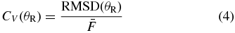
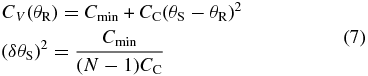
Second, the Coefficient of Variation of the Root Mean Square Deviation, or CV(RMSD) and denoted as CV(θR), provides an absolute, aggregate measure of the differences between the (folded and co-registered) flux data A and  . This symmetry test calculates the sum of the differences squared of the fluxes of pixel pairs that are matched by the reflection operation generally described in Equation (2) and illustrated in Figure 3. At roll angle θR, the root-mean-square deviation (RMSD) of the flux differences of co-registered pixels is therefore

where θ' is the azimuthal offset angle relative to θR, NR is the number of co-registered pixel pairs, and the polar angle ϕ is included only when using the annular sky maps F(θ, ϕ) as input data. CV(RMSD) is then derived using
where  is the mean ENA flux per pixel of all data used to derive RMSD(θR). CV(θR) is always positive, and perfect reflection symmetry corresponds to CV(θR) = 0. While the CV(RMSD) analysis does not yield an explicit correlation coefficient like ρ, its result incorporates the absolute flux differences between A and
  .
.
3.1. Illustrations of Reflection Symmetry
To better interpret the information provided by the symmetry tests, and with some insight into the summary results of this study, we construct the simplest flux symmetries of a circular emission structure that could represent the ribbon flux, shown in Figure 4. Schematically illustrated are a unimodal flux peak in Figure 4(i), opposing bilateral flux lobes of the same flux brightness in Figure 4(ii), partially opposing bilateral flux lobes of different brightness in Figure 4(iii), and non-opposing bilateral flux lobes of different brightness in Figure 4(iv).
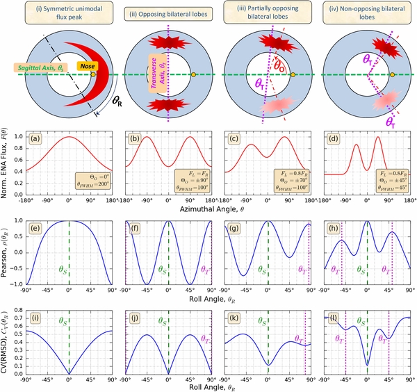
Figure 4. Four general scenarios for the symmetry of the ENA flux distribution around the ribbon are illustrated in panels (i)–(iv), in which blue represents the globally distributed flux and red represents the ribbon flux, analogous to Figure 1. Representative 1D ribbon flux distributions F(θ) for each scenario are shown in panels (a)–(d) using Gaussian distribution(s) superimposed on a constant flux of normalized magnitude 0.35. For each scenario, the symmetry of F(θ) is established using the Pearson correlation coefficient ρ(θR) (panels (e)–(h)) and the CV(RMSD) correlation score CV(θR) (panels (i)-(l)). The sagittal symmetry axis θS (green dashed line) is conveniently selected to lie at θ = 0° and is identified by a global ρ(θR) maximum and global CV(θR) minimum. The transverse symmetry axes θT (purple dotted lines) are identified by local ρ(θR) maxima and local CV(θR) minima.
Download figure:
Standard image High-resolution imageAnalogous to physiological symmetry geometries, we refer to the primary axis of reflection symmetry at θS as the sagittal axis. In Figures 4(i)–(iv), for purposes of illustration in this section, we conveniently select the sagittal axis to lie along the BV-plane, such that the sagittal axis at θS = 0° also corresponds to a roll angle θR = 0°.
For a unimodal flux distribution, a single symmetry axis (the sagittal symmetry axis θS) is observed and is located near the point of bisection of the distribution. For a bimodal flux distribution, we expect to observe up to three axes of symmetry. The sagittal symmetry axis is located where one flux peak is "folded" and co-registered with the other flux peak. The same symmetry operation used to identify θS yields two additional symmetry axes, which we refer to as transverse symmetry axes θT and are located at local ρ(θR) maxima and local CV(θR) minima. Because the symmetry operation applies to the entirety of the ribbon flux, the location of a transverse axis is associated with the internal symmetry of an individual flux peak but is modulated by the global variation of flux around the ribbon. Therefore, a transverse axis can be located near (but not necessarily at) the angle of bisection of an individual flux peak of a bimodal distribution.
Figures 4(a)–(d) show simplistic, 1D azimuthally dependent fluxes F(θ) for each of the scenarios of panels (i)–(iv). These fluxes, analogous to the fluxes FP9(θ) or FP2max(θ) obtained from the IBEX data, are constructed as the combination of the constant, ubiquitous globally distributed flux with normalized flux magnitude 0.35 and an azimuthally varying ribbon flux of one (for unimodal) or two (for bilateral) Gaussian-shaped flux peaks. The parameters of the Gaussian flux distributions are listed in Figures 4(i)–(iv) and include the offset angle ΘO relative to the symmetry axis θS, the angular full-width-at-half-maximum (FWHM) θFWHM, and, for the bilateral peaks, the relative flux magnitudes FL and FR of the left and right flux lobes, respectively.
Figures 4(e)–(h) and Figures 4(i)–(l) show ρ(θR) and CV(θR) calculated as a function of roll angle θR for the flux distribution F(θ) of each scenario. For reference, also shown are the roll angle locations of the sagittal (red dashed line) and transverse symmetry axes (purple dotted line).
As indicated by the autocorrelation analysis of Figure 2, the ribbon flux at lower ENA energies (∼1 keV) likely appears as a unimodal peak that is broad in azimuth. The unimodal Gaussian flux peak of Figure 4(a) is centered at θ = 0°. The Pearson correlation coefficient in Figure 4(e) reaches a single maximum ρ(0°) = +1 (perfect positive correlation) at the sagittal axis and a single minimum ρ(±90°) = −1 (perfect negative correlation) at the transverse axis. The corresponding CV(RMSD) correlation score in Figure 4(i) reaches a single minimum value CV(0) = 0 at the sagittal axis and a single maximum value CV(±90°) = 0.6. A unimodal peak is therefore characterized by (1) a single ρ(θR) maximum and single CV(θR) minimum at the same roll angle, which marks its sagittal axis, and (2) the ρ(θR) minimum and the CV(θR) maximum lie 90° from the sagittal axis.
At 2.7 and 4.3 keV, inspection of the flux maps of Figure 1 and the autocorrelation analysis of Figure 2 clearly indicate the presence of two distinct flux peaks that generally lie on opposite sides of the circular ribbon. We therefore construct in Figures 4(ii)–(iv) three representative (but distinctly different) cases for bilateral flux lobes. The common features across these cases include (1) the flux distribution is the superposition of a constant flux of normalized magnitude 0.35 and two Gaussian flux peaks and (2) the Gaussian flux peaks are symmetrically located at offset angles ±ΘO relative the sagittal symmetry axis, which lies at θ = 0°.
In the first bilateral lobe case, shown in Figure 4(b), the Gaussian bilateral flux lobes are of equal width and magnitude and are offset ΘO = ±90° and are thus on opposite sides of the ribbon, separated by 2|ΘO| = 180°. The two ρ(θR) maxima in Figure 4(f) and two CV(θR) minima in Figure 4(j) indicate strong symmetry along two axes: θR = 0° (the sagittal axis) and θR = ±90° (transverse axis, which is the common symmetry axes that bisects each of the individual opposing flux peaks). Another signature for opposing bilateral lobes is the locations of two pairs of ρ(θR) minimum and CV(θR) maximum at θR = ±45°, midway between the sagittal and transverse symmetry axes.
In the second bilateral lobe case, shown in Figure 4(c), the Gaussian flux lobes are offset ΘO = ±70° from θS and thus referred to as "partially opposing" bilateral lobes. As with the case of opposing bilateral flux lobes, two pairs of ρ maximum and CV minimum are observed. Strong symmetry is present at the sagittal symmetry axis, with ρ(0°) = +1 and CV(0°) = 0.12. However, the second pair of local ρ maximum (at θR ∼ 85°) and local CV minimum (at θR ∼ 74°) are slightly offset from θR = 90° and are not precisely paired at the same roll angle. Additionally, the correlation score CV(74°) at the transverse axis is significantly poorer than the score CV(0°) at the sagittal axis. These are key signatures that distinguish partially opposing bilateral lobes from opposing bilateral lobes.
To illustrate the signatures of bilateral flux lobes of different flux magnitudes, the flux magnitude FL of the left flux peak in Figure 4(c) is 80% that of FR. From Figures 4(g) and (k), this results indifferent magnitudes of the two CV(θR) maxima. Note also that the minimum value of CV(θR) is nonzero, although a nonzero CV(θR) minimum is expected for a natural system in which individual flux peaks are not identical in shape and magnitude.
The third bilateral lobe case, shown in Figure 4(d), has non-opposing flux lobes that are narrow in angular width and separated by 2|ΘO| = 90°. For this case, the two transverse symmetry axes that bisect the individual flux lobes are well-separated and distinct. Therefore, three unique symmetry axes are present and lie near the locations of the three pairs of ρ maximum and CV minimum. As with the other bilateral lobe cases, the sagittal axis lies at the global ρ maximum and CV minimum (θS = 0°), and the transverse axes lie at the roll angles of local ρ(θR) maximum and CV(θR) minimum, which are in the vicinity of the offset angle ΘO of each flux peak.
In summary, the key signatures for interpreting the flux symmetry of the IBEX ribbon include:
- 1.Reflection symmetry is present only when a ρ(θR) maximum and CV(θR) minimum pair lie at the same roll angle θR (Livadiotis & McComas 2013).
- 2.The sagittal symmetry axis is identified at the roll angle of the global maximum ρ(θR) and global minimum of CV(θR).
- 3.The reflection symmetry is strongest when ρ(θR) → +1 and CV(θR) → 0.
- 4.A unimodal peak is characterized by a single, paired ρ maximum and CV minimum, which defines the location of the sagittal symmetry axis. Additionally, the ρ minimum and CV maximum are likewise paired and lie ∼90° from the sagittal symmetry axis.
- 5.Bilateral lobes are characterized by two or three pairs of ρ maximum and CV minimum.
- 6.Opposing bilateral lobes are characterized by two pairs of ρ maximum and CV minimum with similar ρ maxima values and similar CV minima values. The transverse symmetry axis is located ∼90° from the sagittal symmetry axis.
- 7.Partially opposing bilateral lobes are distinguished from opposing bilateral lobes by a single global CV minimum at θS and a local CV minimum at θT, such that CV(θS) < CV(θT). The transverse axis is slightly offset from 90° relative to the sagittal symmetry axis.
- 8.Partially opposing bilateral lobes of different flux magnitudes are identified when the magnitudes of the two ρ minima are dissimilar and the magnitudes of the two CV maxima are dissimilar.
- 9.Non-opposing bilateral lobes are identified by three pairs of ρ maximum and CV minimum.
4. REFLECTION SYMMETRY OF THE IBEX RIBBON: RESULTS
Figure 5 shows the Pearson and CV(RMSD) correlation results for the IBEX data at each energy passband. The points in Figure 5 correspond to calculated values of ρ(θR) (left panels) and CV(θR) (right panels) as a function of roll angle θR, where θR = 0° corresponds to the ribbon center–heliospheric nose vector in the ribbon-centered frame of Figure 1. The red points are derived using FP9(θ) as input data, green points using FP2max(θ), and blue points using the complete 2D flux distribution F(θ, ϕ) of the annular maps of Figure 1. The solid lines through the data points are cubic spline interpolation and are used both to guide the eye as well as a first estimate for identification of the sagittal axis at the global minimum of ρ(θR) and global maximum of CV(θR).
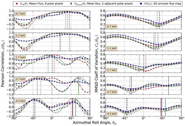
Figure 5. Results for the Pearson correlation analysis (left panels) and CV(RMSD) correlation analysis (right panels) are shown as points for the ENA flux measured by IBEX as a function of roll angle θR relative to the ribbon center–heliospheric nose direction (BV-plane). The error bars of CV(θR) are computed using the IBEX flux variance sky maps (McComas et al. 2014a). The lines connecting the points are a cubic spline interpolation. The black dashed lines that generally follow the FP2max(θ) correlation results are the correlation scores from the double Gaussian fit (Equation (7)) to the FP2max(θ) flux distributions as shown in Figure 8. The vertical dashed lines are the global Pearson correlation maxima and CV(RMSD) minima that indicate the locations of strongest reflection symmetry and thus the sagittal symmetry axis. The solid vertical lines at 2.7 and 4.3 keV mark the locations of the transverse symmetry axes that are distinguishing signatures of bilateral flux lobes.
Download figure:
Standard image High-resolution imageWe find consistently stronger correlation scores (ρ(θR) maxima and CV(θR) minima) for input data FP9(θ) and FP2max(θ) compared to F(θ, ϕ). This is expected because FP9(θ) and FP2max(θ) are average fluxes at each azimuth, whereas F(θ, ϕ) retains the flux variance of nine polar pixels at each azimuth, which is propagated through the correlation calculation and leads to a slightly poorer correlation score. Nevertheless, the F(θ, ϕ) data set provides an important indication of symmetry across the 2D annular flux maps of Figure 1.
4.1. Sagittal Symmetry Axes
To calculate the sagittal symmetry axis locations, we follow Livadiotis & McComas (2013) to identify the Pearson correlation maximum at each energy. We first convert the correlation coefficient to a positive definite quadratic form using R(θR) = 1−ρ(θR)2, such that the maximum positive value of ρ(θR) is located at the same roll angle as the minimum of R(θR). The downward-opening parabola of ρ(θR) near its maximum is therefore transformed into an upward-opening parabola of R(θR) near its minimum. Next, the six data points of R(θR) closest to the estimated symmetry axis (derived from the interpolated roll angle of the ρ(θR) maximum) are fit to

The three fit parameters include: the sagittal symmetry axis θS, which identifies the parabolic vertex; the minimum value Rmin that lies at the parabolic vertex; and the curvature coefficient RC that is used to derive the error of θS. The derived sagittal axes are shown as vertical dashed lines in the left panels of Figure 5 for each input data set FP9(θ), FP2max(θ), and F(θ, ϕ); at each energy, these values are generally clustered together and indicate consistent results over the input data sets.
The errors associated with the derivation of θS from the parabolic fits are crucial for comparing the results across data sets as well as comparing and combining the Pearson and CV(RMSD) results. This error is calculated using the curvature coefficient RC of the fitted parabola according to (Livadiotis & McComas 2013)

where N is the number of data points used for the parabolic fit (here N = 6).
A similar method of parabolic fit and derivation of both θS and δθS are obtained for the CV(θR) results (Livadiotis 2007), whose minimum can intrinsically be modeled in positive definite quadratic form similar to Equations (5) and (6):
where Cmin is the minimum of CV(θR) and CC is the parabolic curvature coefficient. The derived values of θS for the CV(RMSD) results for N = 6 are shown as dashed lines in the right panels of Figure 5 for each of the data sets. At each energy, the sagittal symmetry axes derived using the CV(RMSD) analysis are closely clustered, indicating consistency over the data sets.
In Figure 5, the Pearson correlation results at 2.7 keV for FP9(θ) are unique because three ρ(θR) maxima are observed, with the sagittal axis identified at the location θR ≈ 0° of the ρ(θR) maximum (although a second local maximum of nearly the same magnitude lies at −42°). Additionally, the ρ(θR) minimum lies nearly 90° from the sagittal axis. These are signatures of non-opposing bilateral lobes as indicated in Figure 4(h). However, all other correlation results at 2.7 keV consistently show a sagittal axis near θR ≈ 30°, and none exhibit signatures of non-opposing lobes. We infer from these results that the bilateral lobes at 2.7 keV have only weak signatures of non-opposing flux lobes and, as will be discussed later, are classified as partially opposing lobes. Because of the discrepancy in sagittal axis identification introduced by the signatures of non-opposing lobes, we do not use in any subsequent analysis the value of θS derived using Pearson analysis at 2.7 keV with the FP9(θ) data.
After excluding the Pearson analysis results for the FP9(θ) data at 2.7 keV, we derive the symmetry axis locations θS and their associated errors ±δθS for each energy, each input data set, and both Pearson and CV(RMSD) analyses. These are shown in Figure 6, for which the center black bar at each energy is the composite symmetry axis obtained by combining the Pearson and CV(RMSD) analyses; the Pearson and CV(RMSD) results lie to the left and right of the black bar, respectively. The symmetry axis locations derived using both the Pearson and CV(RMSD) analyses are consistent and clearly show a systematic rotation of θS through ∼65° as the energy increases from 0.7 keV to 4.3 keV.
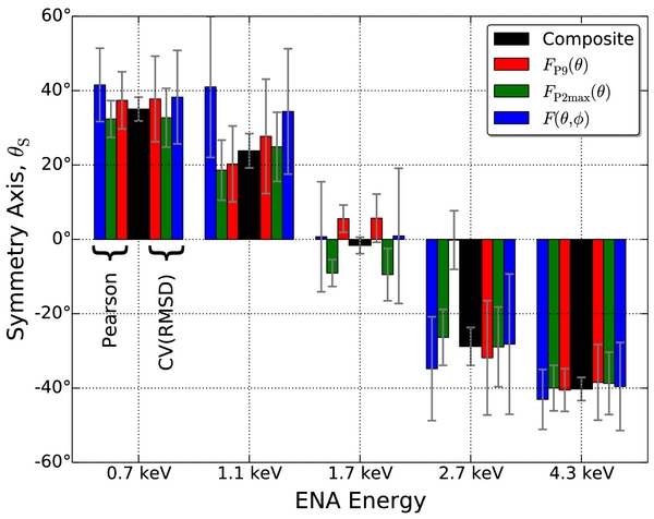
Figure 6. Sagittal symmetry axis angle θS is derived using a parabolic fit to the six data points around the maxima of the Pearson correlation coefficient (left of the black bar at each energy) and the minima for the CV(RMSD) correlation (right of the black bar at each energy). The results are shown for each energy and for each input data set FP9(θ), FP2max(θ), and F(θ, ϕ). The black bar is the composite value of θS from the combined Pearson and CV(RMSD) analyses. The error bars ±δθS are calculated using the parabolic curvature coefficient.
Download figure:
Standard image High-resolution imageAs previously stated, the necessary criteria for identification of strong symmetry and the sagittal axis is the presence of both a maximum of ρ(θR) and a minimum of CV(θR) at a similar roll angle (Livadiotis & McComas 2013). Figure 6 clearly shows that both the Pearson and CV(RMSD) analyses identify consistent locations of θS at each energy, and Figure 5 shows that these values are associated with large, positive values of the Pearson correlation coefficient (∼0.8 to ∼0.95) and small CV(θR) correlation scores (∼0.1 to ∼0.3). This is clear evidence for strong reflection symmetry associated with the ribbon flux.
Table 1 lists the derived weighted mean values of θS (using a weighted mean with weights δθS−2) at each energy for both the Pearson and CV(RMSD) analyses. The Pearson correlation and CV(RMSD) results agree within 3°, which quantitatively demonstrates strong reflection symmetry of the ribbon flux. All Pearson and CV(RMSD) results are then combined at each energy, again using a weighted (δθS−2) average, to obtain a composite value of θS at each energy, which are also listed in Table 1. These values are used as the primary symmetry axes for the remainder of this study.
Table 1. Location of the Sagittal Symmetry Axis θS of the Ribbon Flux Relative to the Ribbon Center–Heliospheric Nose Vector in the Ribbon-centered Frame of Figure 1
| ENA Energy | θS, Pearson Correlation | θS, CV(RMSD) | θS, Composite | Flux Centroid, θF |
|---|---|---|---|---|
| (keV) | ||||
| 0.7 | 350 ± 38 |
352 ± 58 |
350 ± 32 |
27° |
| 1.1 | 214 ± 60 |
272 ± 72 |
238 ± 46 |
24° |
| 1.7 | −18 ± 25 |
−11 ± 46 |
−16 ± 22 |
−3° |
| 2.7 | −283 ± 66 |
−297 ± 81 |
−288 ± 51 |
−18° |
| 4.3 | −409 ± 37 |
−388 ± 57 |
−403 ± 31 |
−9° |
Download table as: ASCIITypeset image
As indicated in Table 1, the sagittal symmetry axis location is a strong function of energy, and we observe systematic rotation from θS = +35° at 0.7 keV to θS = −40° at 4.3 keV. Notably, the sagittal symmetry axes at 0.7 keV and 4.3 keV lie generally on opposite sides of the BV-plane, which is located at θS = 0°.
4.2. Transverse Symmetry Axes
To identify a transverse symmetry axis θT from the data, we use the same parabolic fit method that was used to derive the sagittal symmetry axis: Equation (5) applied to the six closest points around secondary maxima of ρ(θR) or secondary minima of CV(θR). We calculate transverse symmetry axis locations for input data sets that satisfy two criteria: (1) a secondary maximum of ρ(θR) and a secondary minimum of CV(θR) both exist and (2) the peak of the secondary ρ(θR) maximum and trough of the secondary CV(θR) minimum each extend over at least 36° in θR (six 6° pixels) for a meaningful parabolic fit to the data.
The transverse axis locations derived from the parabolic fits are summarized in Table 2 and are shown as the solid vertical lines in Figure 5. As with the derivation of the sagittal axis, the errors δθT of the transverse axis are derived from the curvature coefficient of the parabolic fit, and the composite values of θT are calculated using a weighted mean with weights δθT−2.
Table 2. Location of the Transverse Symmetry Axis θT of the Ribbon Flux Relative to the Ribbon Center–Heliospheric Nose Vector in the Ribbon-centered Frame of Figure 1
| ENA Energy | Input Data Set | θT, Pearson Correlation | θT, CV(RMSD) | θT, Composite | |θT − θS| |
|---|---|---|---|---|---|
| (keV) | |||||
| 2.7 | FP2max(θ) | 629 ± 68 |
594 ± 220 |
626 ± 65 |
914 ± 83 |
| FP2max(θ) | 556 ± 64 |
519 ± 152 |
|||
| 4.3 | FP9(θ) | 480 ± 99 |
415 ± 214 |
518 ± 46 |
921 ± 55 |
| F(θ,ϕ) | 490 ± 137 |
429 ± 240 |
Download table as: ASCIITypeset image
Also listed in Table 2 is the angle between the sagittal (θS) and transverse (θT) symmetry axes. At both energies, the angle between the sagittal and transverse symmetry axes is ∼90°, which is a distinguishing feature of opposing and partially opposing flux lobes.
4.3. Unimodal and Bilateral Flux Distributions
Referring to Figure 5, at 0.71 and 1.1 keV each of the ρ(θR) and CV(θR) correlation distributions exhibits a single maximum and single minimum that are spaced ∼90° apart in roll angle, which is characteristic of a unimodal distribution as in Figures 4(e) and (i). No signatures of bilateral flux peaks are observed at these energies.
At 4.3 keV in Figure 5, two distinct pairs of ρ(θR) maximum and CV(θR) minimum are clearly observed in all data sets, and Table 2 shows that the resulting sagittal and transverse symmetry axes are separated by ∼90°. These are signatures of opposing or partially opposing bilateral flux lobes. Furthermore, the global minimum CV(θS) at the sagittal symmetry axis is approximately half the value CV(θT) at the local minimum of the transverse axis; this notable difference CV(θS) ≪ CV(θT) is a key signature of partially opposing bilateral flux lobes, as illustrated in Figure 4(g). Finally, the magnitudes of the two ρ minima are generally similar, and the magnitudes of the two CV maxima are generally similar, indicating bilateral lobes of similar flux magnitudes. We therefore conclude that the ribbon at 4.3 keV is characterized by partially opposing bilateral flux lobes of similar flux magnitudes.
The results at 2.7 keV are consistent with those at 4.3 keV. In Figure 5, the ρ(θR) results clearly show two maxima that are ∼90° apart in roll angle and indicative of bilateral lobes. The CV(θR) results also show the emergence of a second minimum that is paired with a ρ maximum; this transverse symmetry axis is particularly distinct for the FP2max(θ) data, which are listed in Table 2 and lies ∼91° from θS. Finally, partially opposing flux lobes are indicated by CV(θS) ≪ CV(θT), and flux peaks of similar magnitude are indicated by similar values of ρ minima and of CV maxima.
The results at 1.7 keV exhibit a mixture of unimodal and bimodal flux peaks. In Figure 5, the ρ(θR) results show two maxima that are ∼90° apart in roll angle and thus indicative of bilateral lobes. The CV(θR) results show the emergence toward a second minimum, but not a distinct minimum which is required for classification as bilateral flux lobes.
In summary, the ribbon flux is predominantly unimodal at 0.7 and 1.1 keV, predominantly partially opposing bilateral lobes at 2.7 and 4.3 keV, and in a transition state from a unimodal to bimodal distribution at 1.7. Because the transition from unimodal to bilateral flux distributions occurs between 1.1 and 2.7 keV, we fit the natural log function specified in Figure 7 to the data over this span of energies. The resulting fit, shown as the solid red line, suggests a strong ln(E) dependence of θS for these energies, and the sagittal symmetry axis traverses the ribbon center–heliospheric nose vector (and thus the BV-plane) at 1.65 keV.
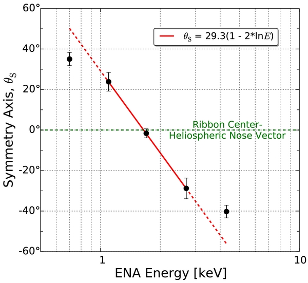
Figure 7. Sagittal symmetry axis locations θS of the ribbon (Table 1, composite values) are a strong function of ENA energy E. The solid red line is a fit of the data at 1.1, 1.7, and 2.7 keV, which span the transition from unimodal to bilateral flux distributions, to a natural log function as specified in the figure. The dashed line shows the fit function extrapolated to 0.7 keV (predominantly unimodal flux distribution) and 4.3 keV (predominantly bilateral flux distribution). The green dashed line shows the ribbon center–heliospheric nose vector, which lies in the BV-plane.
Download figure:
Standard image High-resolution imageThe fit is extrapolated (dashed line) to 0.7 keV, which is a strongly unimodal flux distribution, and to 4.3 keV, which is a strongly bimodal flux distribution. At these energies the extrapolation projects symmetry axes at 50° and −56°, respectively, from the ribbon center–heliospheric nose vector, both of which are ∼15° greater than observed. This indicates that the symmetry axes of the unimodal and bilateral flux distributions are substantially less dependent on energy than at the transition energies; furthermore, the symmetry axis angle may converge toward a single value characteristic of unimodal flux distribution at low energies and, on the opposite side of the ribbon center–heliospheric nose vector (the BV-plane), toward a single symmetry value characteristic of a bilateral flux distribution at high energies.
4.4. Flux Centroid
Presuming the existence of symmetry, a rotationally symmetric flux map, such as opposing bilateral lobes as in Figure 4(ii), results in a flux centroid at the ribbon center. In contrast, a flux distribution that has reflection symmetry but is not rotationally symmetric results in a flux centroid that is displaced from the ribbon center along the sagittal symmetry axis. Examples of such a system include the unimodal flux peak in Figure 4(i), the partially opposing bilateral lobes in Figures 4(iii), and the non-opposing bilateral lobes in Figure 4(iv).
The flux centroid RF relative to the ribbon center for each annular map of Figure 1 is

where ri, Fi, and dΩi are the vector direction, flux value, and solid angle subtended by pixel i in the sky map. If RF lies at the ribbon center, then opposing pixels generally have similar flux, i.e., F(θ) ≈ F(θ + 180°), which is a signature for strong n-fold (n ⩾ 2) rotational symmetry such as opposing bilateral flux lobes (n = 3). Alternately, evidence of strong symmetry in the correlation analysis combined with RF located away from the ribbon center indicates a strong reflection symmetry and weak rotational symmetry, such as a unimodal (n = 1) flux peak or non-opposing bilateral flux lobes. Partially opposing bilateral lobes will also exhibit a centroid, though at a moderate distance from the ribbon center compared to the cases of unimodal and non-opposing flux distributions.
The distance of RF from the ribbon center is a qualitative (rather than a quantitative) indicator of nonrotational ribbon symmetry. Deviation of RF from the symmetry axis can arise from asymmetry of a unimodal flux peak or bilateral flux lobes with different flux magnitudes or different shapes.
Nonribbon flux features that lie within the annular flux maps that do not follow the ribbon symmetry can also influence RF. First, the globally distributed flux is spatially slowly varying, and its total flux in the annular flux maps is a significant fraction (∼0.3–0.5) of the total ribbon flux; a nearly constant flux distributed around the ribbon drives the calculated RF toward the ribbon center. Second, the presence of asymmetric flux variations within the annular maps can drive RF away from the ribbon symmetry axis. This may include asymmetric features of the ribbon flux as well as nonribbon flux features such as the flux from the heliotail (McComas et al. 2013) and the variation of the globally distributed flux (Schwadron et al. 2011, 2014). Therefore, the presence of the globally distributed flux acts to skew RF toward the ribbon center, and asymmetric flux features can skew RF away from the sagittal symmetry axis.
The flux centroids RF calculated using the annular flux maps F(θ, ϕ) of Figure 1 are shown as the points in Figure 8 at each energy. The distance of the centroid points from the center of the plot (the ribbon center) is represented as the fractional distance (in percent) in the polar direction to the polar angle of 745 that was identified in Funsten et al. (2013) as the circular location of maximum ribbon flux at low energies. Also shown as the dashed lines are the composite sagittal symmetry axes θS listed in Table 1. The azimuthal angle θF of RF at each energy is also listed in Table 1 for comparison with the correlation analysis results.

Figure 8. Flux centroid location of the annular ENA flux maps of Figure 1 provides a measure of nonrotational reflection symmetry. The centroid is plotted in the same ribbon-centered frame of Figure 1 as a function of azimuthal angle θ. The centroid distance from the center of the graph corresponds to the fractional distance (in percent) to the average polar angle 745 of maximum circular ribbon flux at low energies (Funsten et al. 2013). The dashed lines are the composite sagittal symmetry axes derived in this study (Table 1).
Download figure:
Standard image High-resolution imageSeveral systematic features of the calculated flux centroids are clearly observed. First, the azimuthal angles of the centroid locations at all energies except 4.3 keV lie within 12° of θS and therefore are consistent with the sagittal symmetry results from the correlation analysis. Therefore, with the exception of 4.3 keV, the abundance of asymmetric flux in the annular maps, which includes the flux variation of the globally distributed flux, is minimal or mutually offsetting (flux of a feature on one side of the ribbon offsets the flux of an independent feature on the other side of the ribbon). The flux centroid at 4.3 keV lies ∼30° from θS, and the annular flux map at this energy likely includes one or more underlying asymmetric flux features that are either not present or exist at lower relative flux magnitude at lower energies.
Second, relative to the sagittal symmetry axis, the azimuthal angle of the flux centroid at each energy is systematically biased toward the ribbon-center heliospheric nose vector (with the exception of 1.7 keV, which lies along this vector and for which θF ≈ θS). This suggests that the predominant asymmetric flux feature(s) in the annular flux maps lie in the vicinity of this vector.
Third, the polar offset of the calculated flux centroid location at 0.7 and 1.1 keV is consistently ∼17% of the characteristic circular radius (745) of the ribbon, while at higher energies is consistently ∼11% of this angular distance. The higher value at lower energies reflects strong unimodal shape; at higher energies, the offset is likely due to partially opposing bimodal flux peak, noting that RF would lie near the ribbon center for opposing bilateral lobes and at a larger angular distance for non-opposing lobes. This result is therefore consistent with the transition from unimodal flux distribution at low energies to partially opposing bilateral flux lobes at higher energies.
5. DISCUSSION
From autocorrelation analysis, Pearson and CV(RMSD) correlation analysis, and flux centroid analysis, we draw compelling evidence of reflection symmetry of the ribbon flux with strong spectral dependence, a transition from a unimodal flux distribution at low energies to partially opposing flux lobes at high energies, and the presence of asymmetric flux features that appear to be aligned with the ribbon center–heliospheric nose vector direction, which, as previously stated, lies in the BV-plane if the ribbon center direction corresponds to  . We now look for global heliospheric ordering of the ribbon symmetry.
5.1. Empirical Representation of the Ribbon Flux Symmetry
With knowledge of the sagittal symmetry axis location θS as a function of energy, we now examine the 1D ribbon fluxes as a function of azimuthal angle Θ from this symmetry axis. Figure 9 shows FP9(Θ) and FP2max(Θ) for −180° ⩽ Θ ⩽ 180°. The FP9(Θ) and FP2max(Θ) flux distributions are generally similar; however, because FP2max(Θ) represents the two highest ribbon flux pixels that are adjacent, FP2max(Θ) is larger and more variable than FP9(Θ).

Figure 9. Ribbon fluxes FP9(Θ) (red circles) and FP2max(Θ) (blue diamonds) are shown as a function of angle Θ from sagittal symmetry axis, which is located at Θ = 0°. The red fill is the average flux  0 of the five lowest-flux pixels in the flux maps of Figure 1; the green fill is the empirical double-Gaussian
  R representation of the ribbon flux (Equation (10)) resulting from the fit of Equation (9) to the FP2max(Θ) flux. The black dashed lines are the individual Gaussian flux peaks of
  R that are equidistant to (but located in opposite directions from) the symmetry axis and whose individual parameters are defined in Table 3. The lines in the bottom panel show the ribbon latitude ΨHCI in the heliocentric inertial (HCI) frame, and the yellow shading corresponds to the band of HCI latitudes associated with the slow solar wind.
Download figure:
Standard image High-resolution imageTo identify systematic trends of the symmetric flux around the ribbon, and for quantitative comparison of the observations of ribbon flux symmetry with models and simulations, we formulate a simplistic empirical representation of the ribbon flux  using
using

We assume that  0 is a constant flux that is independent of Θ and is loosely associated with the globally distributed flux, but does not account for its variation (Schwadron et al. 2011, 2014) in the annular flux maps. At each energy,
  0 is defined as the average flux of the five lowest-flux pixels in the annular flux maps of Figure 1. Values for
  0 are listed in Table 3 and are shown as the red-shaded regions of Figures 9(a)–(e).
Table 3. Fit Parameters Derived from Empirical Fits of Equation (10) to the Data of Figure 9
| ENA Energy |  0 0 |
 |
 |
ΘFWHM1 | ΘFWHM2 | ΘO | fR |
|---|---|---|---|---|---|---|---|
| 0.7 keV | 103 | 360 ± 13 | 405 ± 16 | 154° ± 8° | 128° ± 5° | 61° ± 1° | 3.1 |
| 1.1 keV | 47 | 144 ± 7 | 141 ± 9 | 178° ± 12° | 142° ± 8° | 55° ± 2° | 2.8 |
| 1.7 keV | 27 | 63.0 ± 2.9 | 64.5 ± 1.7 | 85° ± 4° | 187° ± 9° | 68° ± 1° | 1.9 |
| 2.7 keV | 10.6 | 28.6 ± 1.0 | 30.6 ± 0.9 | 112° ± 6° | 125° ± 6° | 74° ± 1° | 2.0 |
| 4.3 keV | 3.8 | 10.1 ± 0.4 | 8.9 ± 0.4 | 118° ± 9° | 129° ± 11° | 79° ± 1° | 1.8 |
Note. ENA fluxes  0,
0,  R1, and
  R2 are in units of (cm2 s sr keV)−1.
Download table as: ASCIITypeset image
The ribbon flux  R(Θ) is constructed as the superposition of two flux peaks of different width and magnitude, but offset by the same distance |ΘO| in opposite directions relative to the sagittal symmetry axis. This construct allows representation of bilateral lobes with reflection symmetry in which the two flux peaks are separated by ∼2|ΘO|. It also allows for a unimodal distribution, when flux peaks with small offset |ΘO| relative to their angular widths merge into a single peak. However, representing the unimodal representation with two unimodal distributions is overdetermined (with complete degeneracy at ΘO = 0°), and small asymmetries in a unimodal flux peak can drive large differences in the fit parameters of the two peaks that comprise
  R(Θ).
R(Θ).
For each of the two ribbon flux peaks of  R(Θ), we use a Gaussian distribution, which has the key parameters of flux magnitude
  R, offset angle ΘO, and distribution width ΘW:
Here,  and
and  are flux constants of each flux peak, ΘW1 and ΘW2 are the Gaussian widths of each flux peak, and ΘO is the azimuthal offset angle of maximum flux relative to the sagittal symmetry axis ΘS. The FWHM for a Gaussian distribution is ΘFWHM = 2.35ΘW.
At each energy, Equation (9) was fit to the FP2max(Θ) data, which are more sensitive to variations in ribbon flux than FP9(Θ) data. The fit parameters are listed in Table 3, the black dashed lines of Figures 9(a)–(e) show the individual flux peaks of  R(Θ), and the green-shaded regions of Figures 9(a)–(e) show the combination of the individual ribbon peaks
  R(Θ).
R(Θ).
The last column of Table 3 lists the ratio fR of the total ribbon flux  (the area shaded green) to the total flux
  (the area shaded red). The ribbon flux clearly dominates at all energies, ranging from a factor of ∼3 larger than the underlying flux at low energies and a factor of ∼2 at high energies.
Several trends are apparent in Figure 9 and Table 3. First, the flux magnitudes  and
and  of the bilateral lobes are similar at each energy, which is consistent with the Pearson and CV(RMSD) analysis results of bilateral lobes with similar flux magnitudes.
Second, the offset angle ΘO of the two lobes increases from ∼60° at low energy to ∼80° at high energy. This increase in offset angle is expected as the flux distribution transitions from a unimodal to a bimodal distribution.
Third, the angular widths ΘFWHM1 and ΘFWHM2 vary substantially over the lowest energies at which a unimodal flux distribution dominates. This results from the overdetermined model  , which is attempting to fit two flux peaks to the unimodal data. Nevertheless, at 0.7 keV and 1.1 keV the resulting fit distribution
  suggests a broad unimodal peak with a slight asymmetry, yielding a maximum flux at Θ ∼ −45° rather than at the sagittal symmetry axis. This is consistent with the slight offset of the flux centroid from the sagittal symmetry axis toward the BV-plane.
The results at 1.7 keV mark the transition from a unimodal distribution to bilateral lobes. However, because the bilateral lobes are emerging and not dominant, this system remains largely overdetermined with the emergence of a bilateral lobe at Θ ∼ 60° driving the fit that results in ΘFWHM1 ≫ ΘFWHM2. Importantly, the results presented here using a bimodal flux model cannot distinguish whether the observed ENA unimodal and bilateral flux distributions result from a single energy-dependent process or a combination of independent processes that operate at different energies.
Fourth, the bilateral flux peaks at 2.7 and 4.3 keV become distinct, and the fit parameters of the two model flux peaks of  R(Θ) agree within 15%. This reinforces the strong reflection symmetry and partially opposing locations that were obtained by the correlation analysis. At these highest energies, the largest deviation of the model results
  R(Θ) from the FP2max(Θ) data lie near the one side of the transverse axis Θ ≈ −90°. At this location, which corresponds to the most northern extent of the ribbon in heliographic latitude, one flux lobe appears to split into two sublobes or, equivalently, a notch of flux depletion appears in the lobe.
Most ribbon models (e.g., Schwadron & McComas 2013) (1) attribute the source population of the ribbon ENA flux to the solar wind and its processing in the heliosheath and (2) assume or derive by modeling that the journey of ENAs from their source to IBEX uniquely retains information about properties of the source plasma. Therefore, we should expect some imprint of the latitudinal structure of the solar wind on the ribbon symmetry or at locations of ribbon asymmetry, and particularly in the vicinity of heliospheric latitude transition between slow and fast solar wind.
Figure 9(f) shows the latitude ΨHCI of the ribbon in the Heliocentric Inertial (HCI) frame (Fränz & Harper 2002), color-coded for energy and assuming, as before, the ribbon is located 745 from the ribbon center. The yellow shaded region corresponds to the HCI latitudes generally associated with the slow solar wind, for which we have used ΨHCI ∼ 36° as the latitude of transition between slow and fast solar wind, although this interface location is substantially blurred by solar variability and by the offset of the Sun's global magnetic field orientation and its spin axis (McComas et al. 2000).
At low energies, we find no obvious association between the symmetry axis of the unimodal distribution and heliocentric latitude. However, at 2.7 and 4.3 keV, we observe that one lobe lies at the highest northern extent of the ribbon, well within the latitude of the fast solar wind, while the other lobe lies at the most southern extent of the ribbon, largely embedded in the region of slow solar wind but reaching the transition latitude between slow and fast solar wind. Therefore, the transverse symmetry axes at 2.7 and 4.3 keV, which lie nearly perpendicular to the sagittal axis, scribe a circle of fixed HCI longitude through the ribbon center. We further investigate this symmetry in the next section.
5.2. Implications and Constraints of Ribbon Symmetry
As viewed from the inner heliosphere, the sagittal symmetry axis is an arc segment of a great circle in the sky that traverses the ribbon center. We therefore represent the symmetry axis as a symmetry plane that contains the Sun and the ribbon center. Figure 10 shows the projection of the symmetry plane (black dashed lines) onto the ENA flux maps in HCI coordinates, whose north pole is tilted 725 relative to ecliptic north and thus is slightly offset from the ecliptic reference frame. Also shown as white diamonds are the location (and its antipode) of the vector normal that defines the symmetry plane. For reference, Table 4 shows one vector normal coordinate (but not its antipode).

Figure 10. IBEX ENA flux maps are shown using a Mollweide projection in heliographic inertial (HGI) coordinates. At each energy, the sagittal symmetry axis derived in Table 1 defines a symmetry plane that scribes a great circle in the sky (dashed black lines). Also shown are the ribbon center (white star) and, as white diamonds, the normal vector to the symmetry plane (also listed in Table 4) and its antipode. For reference, the heliospheric nose and tail directions as well as the locations of Voyagers 1 and 2 are shown as black stars. The ribbon center at ecliptic (2210, 390) lies at HCI (1409, 346).
Download figure:
Standard image High-resolution imageTable 4. Key Parameters of the Sagittal Symmetry Plane of the Ribbon in the Heliocentric Inertial (HCI) Frame
| ENA Energy (keV) | Vector Normal to Symmetry Plane | Tilt of Symmetry Plane Relative to HCI Equator | |
|---|---|---|---|
| HCI Longitude | HCI Latitude | ||
| 0.71 | −113° | 22° | 678 |
| 1.1 | −105° | 31° | 591 |
| 1.7 | −80° | 48° | 423 |
| 2.7 | −37° | 55° | 347 |
| 4.3 | −18° | 53° | 366 |
Download table as: ASCIITypeset image
Table 4 also lists the tilt angle of the symmetry plane relative to the HGI equator. Because the symmetry plane contains the ribbon center, the tilt angle must always lie between a maximum value of 90°, which corresponds to a symmetry plane that contains the HGI poles, and a minimum value of 346, which corresponds to the HCI latitude of the ribbon center. The derived tilt angles of the symmetry plane systematically shift from a maximum of 68° at low energies to ∼35° at 2.7 keV and 4.3 keV.
Since the ribbon center direction indicates, in principle, the interstellar field direction, this result suggests that the symmetry planes define stages in the deformation of the interstellar magnetic field around the heliosphere. The mean free path of ENAs sampled by IBEX is larger at higher ENA energies, thus higher energy ENAs contain information of ENA emission from larger distances from the Sun compared to lower energy ENAs. Therefore, the energy-dependent deflection of the ribbon center (Funsten et al. 2013) and energy-dependent symmetry axes locations are both likely signatures of the magnetic field deformation at different distances from the Sun, with the higher energy ENAs sampling deeper into the ISM where the ISM magnetic field is less perturbed by the heliosphere.
We find an interesting heliospheric latitudinal ordering at 2.7 and 4.3 keV that was qualitatively discovered in Figure 9, in which the tilt angle of the symmetry plane lies within 2° of the heliographic latitude of the ribbon center. Thus, the symmetry plane corresponds closely to the heliographic equator tilted up to the location of the ribbon center. The bilateral flux lobes at these energies therefore lie at the most southern and northern latitudes scribed by the ribbon and may provide insight into the deformed interstellar magnetic field at comparatively large distances from the heliosphere.
Figure 11 shows simulations of the ENA flux that would be measured in the inner heliosphere based on the secondary emission hypothesis (McComas et al. 2009b; Chalov et al. 2010; Heerikhuisen et al. 2010; Schwadron & McComas 2013; Möbius et al. 2013). The ENA flux results are computed by post-processing 3D, time-dependent, MHD-plasma/kinetic-neutral simulation results of the heliosphere based on the Multi-Scale Fluid-Kinetic Simulation Suite (MS-FLUKSS) framework (Pogorelov et al. 2008b, 2009; Heerikhuisen et al. 2013; Zirnstein et al. 2014). The interstellar magnetic field magnitude and direction at the simulation boundary (∼1000 AU) are 3 μG and ecliptic (45°, −44°), respectively. The results are simulated at a measurement time of 2009.5, with solar wind boundary conditions derived from latitudinal and time-dependent equations from Sokół et al. (2013), while accounting for the delay times between primary ENA creation and secondary ENA detection at 1 AU (see Zirnstein et al. 2014 for more explanation).

Figure 11. Simulations of the ENA flux that would be observed at IBEX based on the "secondary" ENA emission hypothesis. The ENA flux, which represents a snapshot in time using solar wind boundary conditions at time 2009.5 (Zirnstein et al. 2014), is shown centered on ecliptic (225°, 44°), which is the antipode of the interstellar magnetic field vector direction used in the simulation. (a) The ribbon at 1.1 keV follows a unimodal distribution that is centered near the BV-plane. (b) At 2.7 keV, the ribbon is predominantly bilateral flux lobes, whose symmetry axis generally lies at the intersection (dashed yellow line) of the ribbon and the equatorial plane (solid yellow line). For reference, the black circle lies at 745 from the ISM magnetic field vector, which is the nominal location of the ribbon relative to the ribbon center (Funsten et al. 2013).
Download figure:
Standard image High-resolution imageThe simulations show circular arcs of ENA flux that generally coincide with the location of the ribbon in the IBEX ENA flux maps. At 1.1 keV shown in Figure 11(a), the ribbon flux is distinctly unimodal and peaked close to the BV-plane, which lies along the ribbon center–heliospheric nose direction. The unimodal ribbon flux distribution that is a dominant feature in the simulation output is directly attributed to the slow solar wind as the primary source population. Furthermore, alignment with the BV-plane indicates the strong, coupled influences of hydrodynamic interactions that are ordered by the direction of the Sun's motion through the ISM and processes that are driven by the ISM magnetic field.
By 2.7 keV, the ribbon flux is distinctly bimodal, with partially opposing bilateral lobes as shown in Figure 11(b). In the simulation, these bilateral flux lobes result from fast solar wind that is associated with higher heliographic latitudes feeding the high latitude extents of the ribbon. The substantial difference between the bilateral lobe flux magnitudes of the simulation results are based on the solar wind properties for the selected epoch up to 2009.5. For example, simulation results using solar wind boundary conditions at time 2013.5 indicate an opposite flux magnitude asymmetry in which the northern lobe is brighter than the southern lobe (see Figure 4 in Zirnstein et al. 2014). These results, which are the subject of a future study, predict that the intensities of bilateral lobes change with the evolution of the solar wind structure and properties over the solar cycle. Nevertheless, this flux magnitude asymmetry of the lobes is notably different than the observations, for which the lobe fluxes are similar in both shape and magnitude. We note that the Figure 1 flux maps used for this study have been acquired over five years, during which the asymmetric brightness of the bilateral lobe fluxes may dynamically change.
Also shown in Figure 11(b) is the equatorial plane (solid yellow line) as projected in the ribbon-centered frame. The bilateral flux lobes appear to be symmetric at the dashed yellow line, which connects the ribbon center and the point of intersection of the equatorial plane and the ribbon. This dashed line marks the inferred symmetry axis and lies below the BV-plane. This is consistent with the 2.7 and 4.3 keV results of Figure 10 in which the symmetry axis corresponds to a tilt of the HCI equator to the ribbon center and suggests a heliographic ordering of the ribbon at high energies.
The ribbon flux is extraordinarily circular and large, spanning ∼150° as projected in the sky (Funsten et al. 2013). This study reveals strong, spectral-dependent reflection symmetry in which the ribbon flux distribution is predominantly unimodal at low energies and predominantly bilateral lobes at high energies. While we find symmetry signatures associated with the HCI reference frame that might be associated with a deformed interstellar magnetic field outside the heliosphere, we do not find symmetry signatures uniquely associated with slow and fast solar wind. This suggests that the ribbon flux is governed by at least one strong spectral filtration process that acts on ENAs between their origin in a source plasma population and their eventual detection by IBEX.
Outside of the ribbon, the spectral information of IBEX measurements may contain more direct signatures of the source plasma properties; for example, ENA spectral measurements at the locations of Voyager 1 and 2, whose locations projected in the sky are largely outside of the ribbon, suggest contributions from multiple plasma populations (Desai et al. 2014). However, the spectral content within the ribbon, which may also contain the combined signatures of multiple plasma populations, are substantially altered by spectral filtration. Thus, understanding the source plasma populations inferred by ENA spectral measurements within the ribbon requires a global understanding of the kinematic processes and energy-dependent transmittance that underlie this spectral filtration.
Key Conclusions:
- 1.The ribbon of ENA flux observed by IBEX has strong reflection symmetry from 0.7 to 4.3 keV, and the primary (sagittal) symmetry axis is a strong function of ENA energy. This study only examines the intrinsic symmetry of the circular ribbon in which the symmetry axis traverses the ribbon center.
- 2.The ribbon ENA flux distribution is predominantly unimodal at 0.7 and 1.1 keV and strongly bimodal, with partially opposing bilateral flux lobes of similar magnitude, at 2.7 and 4.3 keV. The bimodal flux lobes emerge at 1.7 keV. Simulations attribute the slow solar wind as the source plasma for the unimodal flux distribution and the fast solar wind as the source plasma for the bilateral flux lobes.
- 3.The simulations predict asymmetric variability of the flux magnitudes of the bilateral flux lobes over a solar cycle. While the observed flux magnitudes of the bilateral flux lobes are similar, the IBEX flux maps are an integral measurement over a five-year acquisition, which is sufficiently long to mask temporal variability on the time scale of the solar cycle. Flux variability of the bilateral lobes will be an important test for the "secondary" hypothesis of ribbon formation.
- 4.The ribbon center–heliospheric nose vector (and thus the BV plane if the ribbon center defines
 ) appears to be an organizing direction for some symmetry observations. This may indicate the superposition of symmetries associated with the hydrodynamic interaction of the Sun's motion through the ISM, which is ordered by Sun, and the interstellar magnetic field, which is ordered by the direction to the ribbon center. The sagittal symmetry axis appears to be ordered according to the log of the ENA energy, and this ordering appears to be centered at the ribbon center–heliospheric nose direction. First, the sagittal symmetry axes of the unimodal flux distribution at 0.7 and bilateral lobes at 4.3 keV are offset ∼30° in azimuth but in opposite directions from the BV-plane. Second, the sagittal symmetry axis at 1.7 keV, the transition energy between unimodal and bilateral lobe flux distributions, lies in close proximity to the BV-plane. Additionally, the flux centroid analysis indicates that asymmetric flux contributions to the ribbon are biased at ribbon locations in the vicinity of the ribbon center–heliospheric nose vector.
 - 5.The most striking association of ribbon symmetry with the heliocentric inertial (HCI) reference frame is that the sagittal symmetry planes at 2.7 and 4.3 keV correspond to a tilt of the HCI equator to the ribbon center, such that the bilateral flux lobes are located at the northernmost latitudes (ΨHCI ∼ +71°) and extreme southernmost latitudes (ΨHCI ∼ −40°) scribed by the ribbon. The shapes, magnitudes and locations of the bilateral lobes are similar at each energy (with the exception of a flux notch at the transverse axis in the northern lobe).
- 6.The energy dependence of the unimodal and bimodal flux distributions, their locations around the ribbon, and the lack of direct correspondence of symmetry features with fast and slow solar wind strongly suggest the presence of one or more spectral filtration processes that occur between the initial formation of an ENA in the source plasma and its eventual detection at IBEX. The strong dependence of ribbon symmetry on ENA energy may reflect the evolving structure of the perturbed interstellar magnetic field with distance from the Sun. Understanding the underlying processes of spectral filtration is critical for interpreting the observed ENA spectral distributions within the ribbon.
- 7.The different symmetries observed at low (0.7 and 1.1 keV) versus high (2.7 and 4.3 keV) energies may change over time as the structure and properties of the solar wind evolve through the solar cycle.


We gratefully acknowledge all of the contributions made by the entire IBEX team who have been and continue to make this mission a tremendous success. IBEX and this work were funded by NASA as a part of the Explorer Program. Work at Los Alamos National Laboratory was performed under the auspices of the US Department of Energy. M.B. was supported by Polish National Science Center grant 2012-06-M-ST9-00455.