


ABSTRACT
Pickup ions (PUIs) in the outer heliosphere and the local interstellar medium are created by charge exchange between protons and hydrogen (H) atoms, forming a thermodynamically dominant component. In the supersonic solar wind beyond >10 AU, in the inner heliosheath (IHS), and in the very local interstellar medium (VLISM), PUIs do not equilibrate collisionally with the background plasma. Using a collisionless form of Chapman–Enskog expansion, we derive a closed system of multi-fluid equations for a plasma comprised of thermal protons and electrons, and suprathermal PUIs. The PUIs contribute an isotropic scalar pressure to leading order, a collisionless heat flux at the next order, and a collisionless stress tensor at the second-order. The collisionless heat conduction and viscosity in the multi-fluid description results from a non-isotropic PUI distribution. A simpler one-fluid MHD-like system of equations with distinct equations of state for both the background plasma and the PUIs is derived. We investigate linear wave properties in a PUI-mediated three-fluid plasma model for parameters appropriate to the VLISM, the IHS, and the solar wind in the outer heliosphere. Five distinct wave modes are possible: Alfvén waves, thermal fast and slow magnetoacoustic waves, PUI fast and slow magnetoacoustic waves, and an entropy mode. The thermal and PUI acoustic modes propagate at approximately the combined thermal magnetoacoustic speed and the PUI sound speed respectively. All wave modes experience damping by the PUIs through the collisionless PUI heat flux. The PUI-mediated plasma model yields wave properties, including Alfvén waves, distinctly different from those of the standard two-fluid model.
Export citation and abstract BibTeX RIS
1. INTRODUCTION
Most of the heliosphere by volume is partially ionized with the number density of neutral hydrogen (H) greater beyond ∼10 AU than that of the solar wind plasma (Zank 1999; Zank et al. 2013; Heerikhuisen et al. 2014). The collisional charge exchange mean free path in the outer heliosphere ensures that we do not have to directly couple neutral H and the solar wind plasma. However, neutral H in the outer heliosphere is responsible for the creation of pickup ions (PUIs) that eventually form a thermodynamically dominant component of the plasma despite being relatively tenuous. When PUIs are present, they typically play a critical role in almost all facets of the underlying plasma physics.
Several efforts have been made to incorporate PUIs in a self-consistent manner into models that describe the solar wind. A number of models, summarized in Zank (1999), from the 1970s (see especially Holzer 1972; Wallis 1971 for example) assumed a single component background plasma into which pickup protons were added via source terms in the continuity (assuming photoionization), momentum, and energy equations. A more formal derivation of the one-fluid model for the supersonic solar wind mediated by PUIs was provided by Khabibrakhmanov et al. (1996) based on a guiding center kinetic equation derivation. An important extension to the one-fluid models of the supersonic solar wind was introduced by Isenberg (1986). The one-fluid models assume essentially that wave–particle interactions (and particle collisions) proceed sufficiently quickly that PUIs are almost immediately assimilated into the thermal solar wind, becoming indistinguishable from thermal solar wind protons. The one-fluid model of the solar wind predicts a substantial increase in the plasma temperature or pressure (see, e.g., Figure 4.2 of Zank 1999) with increasing heliocentric distance. Such an increase in the temperature of solar wind protons is not observed in the outer heliosphere (Gazis et al. 1994; Richardson et al. 1995) since the Voyager plasma instrument cannot measure PUIs, but a modest increase in the thermal proton plasma temperature is found beyond about 20 AU. The modest temperature increase is due to the dissipation of PUI-generated turbulence (Williams et al. 1995; Matthaeus et al. 1999; Smith et al. 2001; Isenberg et al. 2003; Isenberg 2005; Smith et al. 2006, see also the three-dimensional (3D) models by Kryukov et al. 2012; Usmanov et al. 2014). Instead, as noted by Vasyliunas & Siscoe (1976) and Isenberg (1986), PUIs are unlikely to be assimilated into the supersonic solar wind. Pre-existing and PUI-excited waves will isotropize and stabilize the new-born PUI distribution to produce two approximately co-moving proton populations.
Coulomb collisions are necessary to equilibrate a background thermal plasma, such as the solar wind, and the PUI protons. Let us consider the general case of a background Maxwellian plasma comprised of thermal protons (denoted by the subscript s) and electrons (denoted by the subscript e). PUIs (denoted by the subscript p) then satisfy the ordering
where vts/e denotes the background proton/electron thermal speed respectively and vp the PUI speed. Denoting quantities derived from the background Maxwellian proton or electron distribution with the subscript "b = s/e," the collisional frequency for PUIs is given by (e.g., Zank 2013)
where xb ≡ v/vtb, xp ≡ v/vtp, and  is the thermal speed, Tp/b is the PUI/background electron or proton temperature, nb the background electron or proton number density, ε0 the permittivity of free space, e the electron charge, ln Λ the Coulomb logarithm (∼20), and mp/b the PUI/proton or electron mass. The function G(x) is the Chandrasekhar function for which
For PUIs scattering collisionally off a Maxwellian distribution of background protons, the collision frequency becomes (using the large argument approximation of the Chandrasekhar function)
illustrating the well-known v−3 dependence with PUI speed. By contrast, PUI collisional scattering off a Maxwellian electron background yields a larger collision frequency, which is given by

after using the small argument approximation to the Chandrasekhar function. If the collisional timescale exceeds the characteristic flow time of the plasma region of interest, τf ≃ L/U, where L is the size of the region and U the characteristic velocity, then the PUI distribution will not equilibrate with the background plasma. Expressions (2) and (3) are necessary to determine whether one needs to introduce a model that distinguishes the PUIs from the background plasma protons. In the case of the supersonic solar wind, Isenberg (1986) used related arguments to justify the introduction of a form of multi-fluid model to describe a coupled solar wind–PUI plasma. Isenberg (1986) assumed that PUIs and the solar wind plasma are perfectly co-moving, i.e., Up = Us, where Up is the PUI bulk velocity and Us the thermal solar wind proton bulk velocity. This assumption corresponds to assuming instantaneous isotropization of the PUI distribution at the time of creation. While a reasonable approximation when considering the effects of PUIs on a large-scale flow such as the supersonic solar wind, to understand the impact of PUIs on the basic plasma physical system requires that the PUI-scattering timescale not be neglected. As we discuss below, in the distant outer heliosphere, PUI scattering yields a dissipative collisionless heat flux and viscosity in a collisionless coupled thermal plasma–PUI system. In the inner heliosheath (IHS) regions, the electron heat flux is expected to dominate.
Here, we consider three specific environments in which PUIs mediate the plasma properties: the supersonic solar wind in the outer heliosphere beyond ∼10 AU, the subsonic solar wind, i.e., the plasma in the IHS, and the plasma in the very local interstellar medium (VLISM). Each of these regions is mediated by PUIs, but the origin of the PUI population in each region is different in important ways. We discuss each in turn.
Supersonic solar wind beyond 10 AU. Interstellar neutral gas flows relatively unimpeded into the heliosphere, possibly experiencing some "filtration" at the heliospheric boundaries. Neutral interstellar hydrogen is especially susceptible to the effects of filtration, being decelerated and heated in passing from the VLISM into the heliosphere. The velocity of the neutral H drifting into the supersonic solar wind across the heliospheric termination shock is ∼23 km s−1 or less after filtration in the heliospheric boundaries (Zank et al. 1996b, 2013). The interstellar neutral gas flowing into the supersonic solar wind can be ionized by either solar photons (photoionization) or solar particles (charge exchange, electron-impact ionization, etc.) and the new ions are accelerated almost instantaneously by the motional electric field of the solar wind, E = −U × B, where U is the solar wind flow velocity and B the ambient interplanetary magnetic field (IMF). In a Cartesian frame co-moving with the solar wind, the velocity of a pickup ion is simply v(t) = (− U⊥cos Ωit, U⊥sin Ωit, U∥), where the IMF is oriented along  , U∥ is parallel to
  , U⊥ is perpendicular to
  , and Ωi ≡ qB/m is the local pickup ion gyrofrequency (q denotes charge and m ion mass). The pickup ions therefore form a ring-beam distribution on the timescale
  that streams sunward along the magnetic field. Newly created pickup ions can therefore drive a host of plasma instabilities (e.g., Lee & Ip 1987; see Zank 1999 for a summary). Since the variation in both U and B in the outer solar wind can be substantial, the ring beam should be broad, although this is not assumed typically when investigating related instabilities. PUIs experience scattering and gradual isotropization by either ambient or self-generated low-frequency electromagnetic fluctuations in the solar wind plasma. Since the newly born ions are eventually isotropized, their bulk velocity is now essentially that of the solar wind, i.e., they advect with the solar wind flow, and are then said to be "picked up" by the supersonic solar wind. The isotropized pickup ions form a distinct suprathermal population of energetic ions (∼1 keV energies) in the solar wind whose origin is the interstellar medium (ISM; e.g., Holzer 1972; Lee & Ip 1987; Williams & Zank 1994; see Zank 1999 for an extensive review).
At 10 AU, the number density of PUIs is about 5% of the background thermal solar wind ions, with the fraction increasing to perhaps as much as 20% in the vicinity of the termination shock at ∼90 AU. For the supersonic solar wind at 10 AU, we take the background proton and electron number density to be approximately ns/e ∼ 0.08 cm−1 and the PUI speed to be ∼400 km s−1. This yields a PUI–proton collision time  s. Although the proton number density decreases as r−2 with increasing heliocentric radius r, we may nevertheless compare this collisional time with the convection time of a solar wind parcel from 10 AU to 90 AU, which is τf ∼ 3.38 × 10⁷ s. Clearly, in the supersonic solar wind PUI–proton collisions cannot equilibrate the two proton populations. For PUI–electron collisions at 10 AU, we assume an electron and proton temperature, Ts ∼ Te ∼ 20,000 K. Consequently,
  , which is ∼30 times greater than the characteristic supersonic flow time τf. These estimates neglect the decreasing solar wind number density with increasing heliocentric distance and the possibility that electrons are hotter than solar wind protons, both of which will increase
  . Thus, neither proton nor electron collisions can equilibrate a PUI-thermal solar wind plasma in the supersonic solar wind before the heliospheric termination shock.
The inner heliosheath—the subsonic solar wind. The situation in the IHS, i.e., the region between the heliospheric termination shock (HTS) and the heliopause (HP), is more complicated. The supersonic solar wind is decelerated on crossing the quasi-perpendicular HTS. The flow velocity is directed away from the radial direction and is ∼100 km s−1. The interplanetary magnetic field remains approximately perpendicular to the plasma flow. Voyager 2 measured the downstream solar wind temperature to be in the range of ∼120,000–180,000 K (Richardson 2008; Richardson et al. 2008), which was much less than predicted by simple MHD models. Instead, the thermal energy in the IHS is dominated by pickup ions. There are two primary sources of PUIs in the IHS. The first is interstellar neutrals that drift across the HP and charge exchange with hot solar wind plasma. These newly created ions experience pickup in the IHS plasma in the same way that ions are picked up in the supersonic solar wind. The characteristic energy for PUIs created in this manner is ∼52 eV or ∼6.03 × 10⁵ K, which is about five times hotter than the IHS solar wind protons. The second primary source is the PUIs created in the supersonic solar wind and then convected across the HTS into the IHS. The PUIs convected into the HTS are either transmitted immediately across the HTS or are reflected before transmission (Zank et al. 1996a). PUI reflection was identified by Zank et al. (1996a) as the primary dissipation mechanism at the quasi-perpendicular HTS, with the thermal solar wind protons experiencing comparatively little heating across the HTS. This was confirmed by the Voyager 2 crossing of the HTS (Richardson 2008; Richardson et al. 2008). The transmitted PUIs downstream of the HTS have temperatures ∼9.75 × 10⁶ K (∼0.84 keV) and the reflected protons have a temperature of ∼7.7 × 10⁷ K (∼6.6 keV) (Zank et al. 2010). Clearly, PUIs, those transmitted, reflected, and injected, dominate the thermal energy of the heliosheath, just as PUIs do upstream of the HTS despite being only some 20% of the thermal subsonic solar wind number density. The IHS proton distribution function can be approximated by a three- (Zank et al. 2010; Burrows et al. 2010) or four-component distribution function (Zirnstein et al. 2014), with a relatively cool thermal solar wind Maxwellian distribution and two or three superimposed PUI distributions. In two important papers, Zirnstein et al. (2014) and Desai et al. (2014) have exploited this decomposition of the IHS proton distribution function to great effect in modeling energetic neutral atom (ENA) spectra observed by the IBEX spacecraft at 1 AU (see also Desai et al. 2012, who used the slightly simpler three-distribution model of Zank et al. 2010) to identify multiple proton distribution functions in the IHS and the VLISM. These multiple proton populations are identified as the various PUI populations described above and the thermal solar wind proton population.
For the subsonic solar wind plasma in the IHS, we take the background proton and electron number density to be approximately ns/e ∼ 0.005 cm−1 and the PUI speed to range from ∼1000 (reflected and transmitted PUIs) to 400 (transmitted-only PUIs) to ∼100 km s−1 (PUIs created in the IHS). This yields a lower limit on the PUI–proton collisional time of  s. For an IHS length scale of 100 AU, the characteristic flow time is τf ∼ 1.5 × 10⁸ s. Clearly, in the IHS PUI–proton collisions cannot equilibrate the two proton populations in the upwind region. For PUI–electron collisions, we assume an electron temperature, Te ∼ 200,000 K. Consequently,
  , which far exceeds the characteristic flow time τf on a scale of 100 AU. Thus, neither proton nor electron collisions can equilibrate a PUI-thermal solar wind plasma in the subsonic solar wind or IHS on scales smaller than at least 10,000 AU. For the IHS, a multi-component plasma description that discriminates between PUIs and the subsonic solar wind plasma is therefore necessary. First attempts to write down such a model were presented by Avinash & Zank (2007) and Avinash et al. (2009). Fisk & Gloeckler (2014) have argued similarly that both PUIs and anomalous cosmic rays should be regarded as partially decoupled from the background thermal plasma.
VLISM. the interstellar plasma upwind of the heliopause is also mediated by energetic PUIs. It was noted already by Zank et al. (1996b) that energetic neutral H created via charge exchange in the IHS and fast solar wind could "splash" back into the VLISM where they would experience a secondary charge exchange. The secondary charge exchange of hot and/or fast neutral H with cold (∼6300 K; McComas et al. 2012) VLISM protons leads to the creation of a hot or suprathermal PUI population in the VLISM. The heating of the VLISM has been discussed in detail by Zank et al. (2013), who pointed out that the heating of the VLISM plasma would result in an increase of the sound speed with a concomitant weakening or even elimination of the bow shock (yielding instead a bow wave). Zirnstein et al. (2014) have extended the Zank et al. (2010) model by including the multiple PUI populations that contribute to the heating of the VLISM (Zank et al. 2013). For the purposes of this work, we are concerned primarily with neutrals created in both the IHS and supersonic solar wind, i.e., with typical speeds of ∼100 km s−1 or ∼400 km s−1, experiencing secondary charge exchange in the VLISM. The fast/hot neutrals determine the pickup speed in the VLISM. The PUIs therefore form a tenuous (np ≃ 5 × 10⁻⁵ cm−3; Zirnstein et al. 2014) suprathermal component in the VLISM.
For the VLISM plasma, we take the background proton and electron number density to be approximately ns/e ∼ 0.08 cm−1 and the PUI speed to be ∼100 km s−1 (i.e., H created in the IHS). This yields a lower limit on the PUI–proton collision time of  s. For a length scale of 75 AU, and typical flow speed of 15 km s−1, the characteristic flow time is τf ∼ 7.5 × 10⁸ s. For PUI–electron collisions, we assume an electron temperature, Te ∼ 10,000 K. Consequently,
  , which is comparable to the characteristic flow time τf on a scale of 75 AU. Thus, neither proton nor electron collisions can equilibrate a PUI–thermal plasma in the VLISM on scales smaller than at least 75 AU.
Besides the outer heliosphere and the boundaries with the ISM, the interaction of PUIs with the solar wind is of interest in several planetary environments, both unmagnetized (Venus, Mars, and possibly Pluto), and magnetized (Mercury, Earth (with respect to the AMPTE experiment), Saturn, Jupiter), and at comets (see the review by Coates 2012). For example, PUIs at Venus are created by charge exchange or photoionization from cold neutral ionospheric atoms (e.g., Luhmann 1986). Lu et al. (2013) used Venus Express (VEX) observations to show that the strength of the Venusian bow shock is weaker when PUI production is high. In particular, investigating the interaction of comets with the solar wind has been extraordinarily fruitful in furthering our understanding of PUIs in the solar wind—this includes the missions to Comet Halley and Giacobini–Zinner, and later missions to Grigg–Skjellerup and Borrelly (e.g., Coates 2012). With impending encounters of New Horizons with the Pluto–Charon system (2015) and Rosetta with comet Churumov–Gerasimenko (2014–15), active Venus (VEX) and Mars (Mars Express) missions, and of course Voyager 1 and 2 and IBEX, understanding in more detail the nature of PUI mediated plasmas is of far reaching importance.
The paper is organized as follows. In Section 2, we derive the basic equations describing a PUI mediated plasma. At the first-order, we find that the scattering of PUIs in a turbulent magnetofluid introduces a term analogous to that of heat conduction. The second-order correct set of equations describing PUIs in a multi-fluid context leads to the introduction of the viscous terms that define the PUI stress tensor. We systematically derive the system of multi-fluid equations that describe a background Maxwellian proton and electron plasma plus a non-Maxwellian PUI population. Because we assume Maxwellian distributions for the background protons and electrons, the background plasma contributes no heat flux or stress tensor terms. For completeness, we derive a "single-fluid" description analogous to the equations of magnetohydrodynamics (MHD) that describes a PUI mediated plasma. The "single-fluid" model possesses collisionless heat flux and viscous stress terms, unlike the MHD equations. In Section 3, we derive the dispersion relation for linear waves in a PUI mediated plasma and discuss the general properties of waves in a multi-fluid PUI mediated plasma. In Section 4, we present numerical solutions to the dispersion relation for the supersonic solar wind, the IHS plasma, and the plasma in the VLISM. The multi-fluid waves are also compared to the more familiar two-fluid plasma modes. In Section 5, we present an analysis and numerical solutions of the linearized single-fluid model, presenting results for the VLISM only. In the final section, we discuss and summarize our results.
2. DERIVATION OF THE MULTI-FLUID MODEL
2.1. First-order Correct Multi-fluid Model: Heat Conduction
In deriving a multi-fluid model that includes PUIs self-consistently, we shall assume that the distribution function for the background protons and electrons are each Maxwellian, which ensures the absence of any heat flux or stress tensor terms for the background plasma. The exact form of the continuity, momentum, and energy equations governing the thermal electrons and protons are therefore given by
for the electrons, and
for the protons. Here ne/s, ue/s, and Pe/s are the usual macroscopic fluid variables for the electron/proton number density, velocity, and pressure respectively, γe/s the electron/proton adiabatic index, E the electric field, B the magnetic field, and e the charge of an electron.
Pickup ions initially form an unstable distribution that excites Alfvénic fluctuations. The self-generated fluctuations and in situ turbulence serve to scatter PUIs in pitch angle. The Alfvén waves and magnetic field fluctuations both propagate and convect with the bulk velocity of the system U = U(ue, us, up, ne, ns, np, me, mp), where np and up refer to PUI variables. The PUIs are governed by the Fokker–Planck transport equation with a (for now unspecified) collisional term δf/δt|c,
for average electric and magnetic fields E and B. We assume that the velocity v of PUIs is always non-relativistic. The transport Equation (10) has to be transformed into a frame that ensures there is no change in PUI momentum and energy due to scattering. For the present, assume that the cross-helicity σ is nonzero and let

where VA is the Alfvén velocity and c is the random velocity. The transport equation is therefore
The velocity U is still unspecified, so we choose U such that E' ≡ E + U × B = 0. This assumption corresponds to choosing
since we choose U∥ = 0 (U∥ is parallel to B and therefore arbitrary). This corresponds to expressing (10) in the guiding center frame. The transformation to the velocity U then yields
after setting the cross-helicity σ = 0. By taking moments of (14), we can derive the evolution equations for the macroscopic PUI variables, such as the number density np = ∫fd3c, velocity npupi = ∫cifd3c, and so on. Although unspecified for now, we shall assume that moments of the collisional term δf/δt|c are zero. This can be checked against the particular scattering model that we use below. The zeroth moment of (14) yields the continuity equation for PUIs,
where up is the PUI bulk velocity in the guiding center frame. For the first moment, we multiply (14) by cj and integrate over velocity space. This yields, after a little algebra,
where εijk is the Levi–Civeta tensor.
To close Equation (16), we need to evaluate the PUI distribution function f, which requires that we solve (14). In solving (14), we assume (1) that the PUI distribution is gyrotropic, and (2) that scattering of PUIs is sufficiently rapid to ensure that the PUI distribution is nearly isotropic. We can therefore average (14) over gyrophase, obtaining the so-called focused transport equation for non-relativistic particles (Isenberg 1997). Details of the derivation can be found in Chapter 5 of Zank (2013), and the explicit expression is given in Appendix A. To solve the gyrophase-averaged transport equation requires that we specify the scattering or collisional operator. We make the simplest possible choice, which is the isotropic pitch-angle diffusion operator,
where μ = cos θ is the cosine of the particle pitch-angle θ and  is the scattering frequency. The form of the scattering operator (17) allows us to solve the focused transport equation (A1) using a Legendre polynomial expansion of the distribution function f. This is summarized in Appendix A and details can be found in Chapter 5 of Zank (2013). The first-order correct solution to the gyrophase-averaged form of Equation (14), i.e., (A1), is


where c = |c| is the particle random speed, b ≡ B/B is a directional unit vector defined by the magnetic field, and D/Dt ≡ ∂/∂t + Ui∂/∂xi is the convective derivative. Both f0 and f1 are functions of position, time, and particle random speed c, i.e., independent of pitch-angle μ (and of course gyrophase ϕ). Of particular importance is the retention of the large-scale velocity U acceleration and shear terms. These terms are often neglected in the derivation of the transport equation describing f0 (for relativistic particles, the transport equation is the familiar cosmic ray transport equation). Thus, the second term in (20) is typically neglected, although it is known as the relativistic heat inertia term in the relativistic transport theory of cosmic rays (Webb 1985, 1987, 1989). As will be seen below, retaining these terms is absolutely essential to derive the correct multi-fluid formulation for PUIs. By introducing
we can show that
where
Consequently, the PUI stress tensor is identically zero at first-order and there exists only an isotropic pressure tensor δijPp. We show in the following section that retaining the second-order terms in the Legendre polynomial expansion of the gyrophase-averaged equation (A2) does in fact yield a non-zero collisionless stress tensor. The PUI momentum equation to first-order can therefore be expressed as
To derive the transport equation for Pp, we multiply (14) by (1/2)c2 and integrate over d3c. We then use (18)–(20) to evaluate the various integrals. Introducing c' ≡ c − up as before, we find

for example. Similarly, we find that the heat flux q(x, t) can be expressed as
It then follows that
and
In (25), we introduced the spatial diffusion coefficient
together with PUI speed-averaged form Kij. The collisionless heat flux for PUIs is therefore described in terms of the PUI pressure gradient and consequently the averaged spatial diffusion introduces a PUI diffusion time and length scale into the multi-fluid system. The diffusion coefficient, i.e., the coefficient for the PUI heat flux, is proportional to the particle scattering time τs, and therefore a function of the background turbulent intensity. A separate calculation, possibly based on quasi-linear theory for the parallel diffusion coefficient or the nonlinear guiding center theory for the perpendicular diffusion coefficient, is necessary to obtain reasonable estimates of the scattering time (Matthaeus et al. 2003; Zank et al. 2004).
The remaining terms are straightforwardly evaluated. We find
On combining these results, we obtain, after some algebra, the transport equation for the PUI pressure
illustrating that the PUI heat flux yields a spatial diffusion term in the PUI equation of state. The PUI system of equations is properly closed and correct to the first-order. The second-order correct PUI equations, which includes the PUI stress tensor, is given in the following subsection. For completeness, the PUI total energy equation has the form
The full system of PUI equations is given by (15), (23), and (27) or (28). It is not particularly illuminating to work in the guiding center frame, and we may simplify (15), (23), and (27), (28), by letting
The right-hand side (RHS) of Equations (23) and (28) is proportional to up × B, which becomes
since E was perpendicular to B by construction initially. Hence the PUI fluid equations can be written in the more familiar form
which is the form we use below. Similarly, we have

The full thermal electron-thermal proton–PUI multi-fluid system is therefore given by Equations (4)–(9) and (29)–(31) or (32), together with Maxwell's equations


where J is the current and μ0 the permeability of free space.
2.2. Second-order Correct Multi-fluid Model: the Stress Tensor
As shown above, the zeroth- and first-order solutions for the pressure tensor yields an isotropic scalar pressure Pij = Ppδij only. Consider now the second-order Legendre polynomial expansion of f,
As before, we need to evaluate
from which we find
Although not discussed explicitly above, since the PUI pressure is defined in the frame of the bulk PUI velocity up, the distribution function over which the integral is taken needs to evaluated in this frame. Since the expression (A7) for f2 is a function of the guiding center velocity U, we need to transform to the frame U' = U + up. On using the solution (A7) for f2, we obtain
where the coefficient of viscosity η is defined as
Equation (41) is the formal definition of the coefficient of viscosity for the PUI gas. If we assume (probably reasonably) that |c| ≫ |up|, then we obtain (42), which may be regarded as a PUI pressure moment weighted by the PUI scattering time. Finally, if we assume that τs is independent of c, we then obtain the "classical" form (43) of the viscosity coefficient. The pressure tensor may therefore be expressed as
The pressure tensor may be written in a more revealing form if we introduce a "viscosity matrix,"
and note that ηij = ηji and η/15 = η11 + η22 + η33 = ηijδij (since b2 = 1). Then
which yields the pressure tensor as the sum of an isotropic scalar pressure Pp and the stress tensor, i.e.,
The stress tensor is a generalization of the "classical" form in that several coefficients of viscosity are present, and of course the derivation here is for a collisionless charged gas of PUIs experiencing only pitch-angle scattering by turbulent magnetic fluctuations. Use of the pressure tensor (47) yields a "Navier–Stokes"-like modification of the PUI momentum equation,
where we used Up = up + U ≡ U' as before. The full momentum equation with the second-order stress tensor correction is included for completeness but in the linearized wave analysis below, we use only the first-order correct equations, i.e., only the heat conduction term is included.
2.3. Reduced "Single-fluid" Model
For some problems, such as the investigation of turbulence in the outer heliosphere, IHS, or VLISM, the full multi-fluid model is far too complicated to solve. By making the key assumption that Up ≃ us, we can reduce the multi-fluid system above to an MHD-like set of model equations. The assumption that Up ≃ us is quite reasonable since (1) the bulk flow velocity of a plasma is always dominated by the protons, and (2) the pick-up process itself forces newly created PUIs to essentially co-move with the background plasma flow. Accordingly, we let Up ≃ us = Ui be the overall proton (i.e., thermal background protons and PUIs) velocity. The thermal proton and PUI continuity and momentum equations are therefore trivially combined as
where ni = ns + np. Since the PUIs are not thermally equilibrated with the background plasma (Ts ≠ Tp), we need to deal separately with the Ps and Pp equations. These become
By combining the proton Equations (49)–(52) with the electron Equations (4)–(6), we can obtain an MHD-like system of equations. On defining new macroscopic variables,
we can express
where the smallness of the mass ratio ξ ≡ me/mp ≪ 1 has been exploited. Use of the approximations (54) allows us to combine the continuity and momentum equations in the usual way and to rewrite the thermal electron and proton pressure in terms of the single-fluid macroscopic variables. Thus,
where
Since we may assume that the current density is much less than the momentum flux, i.e., |J| ≪ |ρU|, we can simplify (58) further by neglecting the RHS. By assuming that γe = γs = γ, we can combine the thermal proton and electron equations in a single thermal plasma pressure equation with P ≡ Pe + Ps,
Note that at this point, no assumptions about either the thermal electron or proton pressures (or temperatures) have been made.
Finally, we need an equation for the electric field E. To do so, we multiply the respective momentum equations by the electron or proton charge, sum, and use the approximations (54) to obtain
The generalized Ohm's law is therefore
where we have retained the PUI pressure since in principle it can be a high temperature component of the plasma system and ξPp may be comparable to the Pe term. For our cases of interest, however, Tp ∼ 106 K, Te ∼ 104 K in the supersonic solar wind, Tp ∼ 107 − 108 K, Te ∼ 105 K in the IHS, and Tp ∼ 106 K, Te ∼ 104 K in the VLISM, and np < 0.2ne. Thus, we find that the Pp term can be neglected in Ohm's law (60). Neglect of the electron pressure and Hall current term then yields the usual form of Ohm's law.
The reduced single-fluid model equations may therefore be summarized as


The single-fluid description (61)–(68) differs from the standard MHD model in that a separate description for the PUI pressure (64) is required. The PUIs introduce both a collisionless heat conduction and viscosity into the system. Notice that the derived electric field (65) is consistent with that used in the transformation of the PUI Fokker–Planck equation (10) i.e., the bulk velocity U derived for the reduced system corresponds to that used in the velocity transformation to eliminate the electric field in (10).
The model Equations (61)–(68), despite being appropriate to non-relativistic PUIs, are interestingly related to the so-called two-fluid MHD system of equations used to describe cosmic ray mediated plasmas (Webb 1983). However, the derivation of the two models is substantially different in that the cosmic ray number density is explicitly neglected in the two-fluid cosmic ray model and a Chapman–Enskog derivation is not used in deriving the cosmic ray hydrodynamic equations. Nonetheless, the sets of equations that emerge are the same suggesting that a more careful analysis of the cosmic ray two-fluid equations would show that the system can in fact include the cosmic ray number density explicitly and therefore be capable of describing the full plasma system.
3. LINEAR WAVE ANALYSIS
The PUI mediated plasma model derived above lends itself to a variety of applications. Here, we analyze linear waves in the three regions discussed in the Introduction, viz., the supersonic solar wind in the outer heliosphere, the subsonic solar wind in the IHS, and the VLISM. As we discuss below, the wave properties in these three regions are significantly different from those in the inner heliosphere, which is essentially unmediated by PUI physics. The closest correspondence is to multi-fluid models that include heavy ions as a minority component (Mann et al. 1997; Verscharen et al. 2013), but the heavy ions do not typically dominate the thermal energy budget of the plasma system.
The linearization of the PUI multi-fluid equations proceeds in the standard way and we assume

We seek plane wave solutions ∝exp [i(ωt − k · x)], where ω is the frequency, and k = (kx, 0, kz) the wave number. Some algebra allows us to express the linearized system in terms of the background protons, electrons, and PUI matrices Ms, Me, and Mp through the electric field fluctuations and respective velocity fluctuations,
where
The final relation needed to complete the derivation of the dispersion relation follows from the definition of the current,
where
In Equations (69)–(74), we have introduced the proton gyrofrequency Ωp = eB0/mp, the mass ratio ξ ≡ me/mp, the electron number density n0, the density ratio or concentration α ≡ ns0/n0 and thus np0 = n0(1 − α). The square of the Alfvén speed is defined with the electron number density n0 as
and the thermal proton, electron, and PUI sound speeds are defined as
and γe/s/p refers to the appropriate adiabatic index. Note that the definition of the electron sound speed contains the ratio me/mp. Finally, note that the scalar k · K · k is present in (72). The diffusion tensor is assumed to be of a simple diagonal form (i.e., we do not include the off-diagonal terms associated with drift and curvature—see the discussion in Zank 2013) and we specify

Recall that the formal definition of the heat conduction spatial diffusion coefficient is (see the definitions (25) and (26))
where the ensemble average is taken over characteristic PUI speeds. Accordingly, if we crudely approximate the scattering time by the inverse gyrofrequency, we have κ∥ ≡ 〈c2〉/3Ωp, where 〈c2〉 is an ensemble averaged characteristic speed of the PUIs. We therefore introduce the definitions
and χ = 0.01. In estimating the diffusion coefficients (79), we need to choose a typical PUI speed for the system of interest weighted appropriately according to the definition of K, e.g., in the supersonic solar wind, one might choose 〈c2〉1/2 to be some fraction of 400 km s−1. Although we assume that the scattering time can be approximated by the PUI inverse gyrofrequency, the real scattering time may well be much slower. Our choice of χ = 0.01 is motivated by models of the perpendicular diffusion coefficient derived from nonlinear guiding center theory (Matthaeus et al. 2003), which, when evaluated for explicit turbulence models, yields a ratio of ∼0.01 between the perpendicular diffusion and parallel coefficients (Zank et al. 2004).
From the expression for the current (73), and relations (69) et seq., the determinant is

from which the dispersion relation can be expressed as

The dispersion relation (80) is formidably complicated, containing as a subset the full two-fluid model (Stringer 1963; Sahraoui et al. 2012 and references therein). Nonetheless, neglecting electron inertia yields a somewhat "tractable" 11th-order polynomial dispersion relation, whereas in the limit of small PUI abundance α → 1, electron inertia effects can be retained. These various limits are discussed below.
3.1. Dispersion Relation in the Absence of Electron Inertia
The neglect of electron inertia in (80) yields an 11th-order polynomial dispersion relation,
where the coefficients are given in Appendix B. The entropy mode ω = 0 is already eliminated from the dispersion relation (81). The dispersion relation is written in a form that facilitates expression in dimensionless units, e.g.,  ,
,  and
and  .
.
3.1.1. Parallel Propagation, θ = 0°
On setting θ = 0°, the dispersion relation (81) can be factored into three separate dispersion relations. The first corresponds to dispersive Alfvén waves, i.e., ion-cyclotron or whistler modes satisfying
with solutions
The ion-cyclotron mode satisfies ω → ±Ωp in the limit that k → ∞, whereas the whistler mode satisfies ω → ±∞ in the same limit (since electron inertia is neglected).
The second factorization corresponds to a hybrid proton–PUI mode

The remainder of the polynomial dispersion relation couples the proton and PUI sound modes, and is given by
For the cases that we consider, α is quite close to 1, typically different by some 10%–20%. The dispersion relation is therefore usefully rewritten as
It is easily seen that setting α = 1 yields as solutions to (87), the


In the absence of spatial diffusion, (90) corresponds to a simple PUI sound mode ω = ±Cpk. The second term in (90) is imaginary with positive sign and therefore describes how PUIs also damp the PUI sound mode. For α ≠ 1, the modes (88)–(90) are coupled.
Further insight into (86) is obtained by introducing the phase speed Vp ≡ ω/k. The diffusion term k · K · k can be expressed as κ∥k2 for parallel wave propagation. For a characteristic phase speed V0, we may exploit the length scale introduced by the diffusion coefficient κ∥ to consider long wavelength and short wavelength modes, using either
respectively. On using  ,
,  , the normalized form of (86) becomes
We can solve (92) in the long wavelength limit by setting ε ≡ O(κ∥k/V0) ≪ 1 and using  . Similarly, we can solve (92) in the short wavelength limit using ε ≡ O((κ∥k/V0)−1) ≪ 1 and using
  . For the long wavelength limit, we obtain five solutions, one of which is a purely damped mode
with damping rate proportional to the PUI concentration. Another solution is the PUI acoustic mode that is coupled weakly to the thermal plasma and is diffusively damped,
The final long wavelength limit mode admitted by (92) is a two-fluid acoustic mode that is coupled weakly to the PUIs and is weakly diffusively damped, with
The converse short wavelength limit shows that there is no PUI mode. Only the two-fluid acoustic mode persists and it is very weakly coupled to the PUIs via the concentration (1 − α) and is damped by PUIs. Thus, we have
A second slowly propagating mixed thermal acoustic mode exists, which is also damped by PUIs,
Finally, in the short wavelength limit, (92) admits a purely damped non-propagating mode
3.1.2. Perpendicular Propagation, θ = 90°
The reduced dispersion relation for perpendicularly propagating waves is a fifth-order polynomial,
It is instructive to consider the limit α = 1. In this case, we recover the two-fluid fast mode
together with a third-order polynomial describing the separate propagation of PUI modes,

In this case, the term k · K · k = κ⊥k2. To analyze (101), we again introduce the phase velocity Vp ≡ ω/k and normalize with a characteristic speed V0, and consider the κ⊥k/V0 ≪ 1 and κ⊥k/V0 ≫ 1 limits. The long wavelength limit yields a purely damped PUI mode with
and a damped PUI-cyclotron wave
The short wavelength limit possesses two purely damped modes, one of which is
together with
In the short wavelength limit, we may expand the last expression to obtain the two limiting purely imaginary cases,
Although algebraically tedious, the fifth-order dispersion relation (99) is similarly amenable to an analysis in the long and short wavelength regimes. This has the virtue of identifying the basic couplings of the thermal plasma and PUI components, but is no more revealing of the basic modes than the above analysis. We do not therefore reproduce the analysis for (99).
3.1.3. Oblique Propagation, θ ≠ 0°, 90°
The only limit of the full dispersion equation that is analytically tractable is α → 1. In this case, in the absence of electron inertia, the dispersion relation (81) factors into the standard two-fluid dispersion relation without electron inertia (Stringer 1963; Sahraoui et al. 2012),
and a PUI-only dispersion relation,
The solutions to (107) are the usual dispersive two-fluid modes, viz., slow, fast, and Alfvén modes with the standard properties. The PUI dispersion relation can be solved in the long and short wavelength limits. In the long wavelength regime (using κ ≡ κ∥cos 2θ + κ⊥sin 2θ), we find two solutions for the arbitrary angle θ that yield positive real frequency,
Note that the two plus signs and the two minus signs act in concert. The two quasi-parallel propagating modes in expression (109) are expressed in a more revealing form as
and the two quasi-perpendicular propagating modes as
Finally, the short wavelength limit yields four damped modes, with
At sufficiently small scales (112) is purely damped and becomes
3.1.4. Inclusion of Electron Inertia
The inclusion of electron inertial terms renders the dispersion relation unreasonably large to express as a polynomial, and so we directly solve the linearized system of equations numerically. However, it is illuminating to consider, as before, the limit α → 1. In this case, the entire dispersion relation separates into a two-fluid dispersion relation (Stringer 1963; Sahraoui et al. 2012) and a separate PUI dispersion relation. The two-fluid dispersion relation is the well-known sixth-order polynomial,4 given by
where the coefficients are
In (116), we have introduced the combined thermal plasma sound speed  .
.
The PUI dispersion relation may be expressed as
which, not surprisingly, is identical to (108). In the limit that α = 1, electron inertia therefore modifies only the two-fluid modes. For a non-vanishing pickup ion abundance, all modes are of course coupled and electron inertia modifies all waves.
For parallel wave propagation, solutions of the two-fluid dispersion relation (115)–(116) can be obtained readily. The dispersive Alfvén wave solutions (the ion-cyclotron and whistler modes) are given by

Now, because of the inclusion of electron inertia, the whistler mode frequency is bounded by the electron cyclotron frequency in the limit k → ∞ and ω → ±(Ωp/ξ) = ±Ωe. For the ion-cyclotron mode, the limit k → ∞ yields the same result when electron inertia terms are neglected, i.e., ω → ±Ωp.
Similarly, the two-fluid sound mode is a solution of (115)–(116) with
As in the case with no electron inertia, the hybrid proton-pickup ion mode ω = ±Ωp and the ion-cyclotron and whistler modes (118) and (119) are also solutions of the full linearized coupled system (i.e., without taking the limit α → 1). The limit α → 1 is useful primarily to distinguish the two-fluid sound mode (120) and the pickup ion sound mode (90), which are otherwise coupled.
For perpendicular wave propagation, the fast two-fluid magnetosonic mode is modified by electron inertial effects to read
In the limit k → ∞, the frequency is  .
.
Finally, for obliquely propagating modes, an additional horizontal "resonant" frequency asymptote is introduced, given by ω = Ωecos θ, as is clearly seen in numerical solutions (it is harder to see analytically). It is interesting to note that for purely parallel propagation, it is the fast (whistler) mode that has this limit. However, for oblique propagation (in which case the modes never intersect), the fast mode frequency continues to increase and it is the Alfvén mode that has this limit. For normal propagation angles, this is relevant only at very small scales, but for highly oblique angles (see, for example, our later Figure 1 for θ = 88°), this effect becomes more apparent at larger scales.

Figure 1. Dispersion and damping curves for parameters appropriate to the VLISM, assuming α = 0.999375 and 〈c2〉1/2 = 200 km s−1. In the left and right panels, the horizontal dotted lines correspond to the asymptotes ω = Ωpcos θ and ω = Ωecos θ. Note that our linear analysis uses exp [i(ωt − k · x)] so that damping corresponds to the positive value of the imaginary part of the frequency. Top panel: θ = 0°, two-fluid wave modes (left); three-fluid with diffusion wave modes showing the real frequency (middle), and the damping rate (right). The slow PUI mode is fully damped for wave numbers k ⩾ Ωp/VA. Second panel: θ = 30°, two-fluid (left); three-fluid real frequency (middle), and damping rate (right). Note that the fast PUI mode (black) is evanescent at wave numbers greater than about k ⩾ Ωp/VA. Third panel: θ = 70°, two-fluid (left); three-fluid real frequency (middle), and damping rate (right). Fourth panel: θ = 88°, two-fluid (left); three-fluid real frequency (middle), and damping rate (right). Bottom panel: θ = 90°, two-fluid (left); three-fluid real frequency (middle), and damping rate (right). For the VLISM parameters used here, all modes intersect. Despite the damping of all modes by PUIs in the three-fluid model, for real frequencies the three-fluid model essentially separates into a two-fluid (protons and electrons) and a PUI-fluid model, i.e., the two-fluid solutions (red, green, and blue) are almost identical in the left and middle columns.
Download figure:
Standard image High-resolution image4. SPECIFIC EXAMPLES OF LINEARIZED WAVES IN PUI MEDIATED PLASMAS
4.1. Identification of Modes in the Numerical Solutions
To properly investigate the dispersion relation in full generality appropriate to the three PUI mediated regions of interest (the outer heliosphere, the IHS, and the VLISM), we need to obtain numerical solutions. The previous estimated solutions provide useful guidance to identify modes at the largest and smallest scales and weak concentrations. Considering only positive frequencies at long wavelengths (conveniently defined as in the vicinity of kVA/Ωp = 0.01), we introduce the following colors to correspond to the following (approximate) designation of wave modes. (1) The slow (red) and fast (blue) two-fluid magnetosonic modes:
(2) the Alfvén mode (green):

(3) the slow pickup ion mode (cyan):

and the fast pickup ion mode (black):

For the cases of interest here, the PUI sound speed Cp is larger than both the Alfvén speed VA and combined thermal plasma sound speed  . Thus, for small propagation angles, the order of the modes will always be ωs < ωA < ωf < ωsp < ωfp, i.e., red, green, blue, cyan, and black. However, as θ increases, the frequency of the fast proton (blue) mode increases too with
  and the frequency of the slow pickup ion (cyan) mode decreases with ωsp → 0. Therefore, beyond some critical angle θc, the fast proton mode will be faster than the slow pickup ion mode (i.e., the blue mode will find itself above the cyan mode). This will happen at the critical angle
Furthermore, because ωA < ωsp for all angles θ beyond the critical angle θc the order of the modes will always be ωs < ωA < ωsp < ωf < ωfp, i.e., red, green, cyan, blue, and black. Of course, this is only approximate since we are discussing the strict limits α → 1 and k · K · k → 0. Nevertheless, for our parameters at 10 AU, for example, the critical angle corresponds to θc = 76.71°, which is why it is difficult to correctly identify the cyan and blue modes at 70° in this case. The corresponding angles for the VLISM and the IHS are θc = 71.86° and θc = 79.14°, respectively.
In all three of the particular cases that we consider below, we solve numerically the full dispersion relation including the electron inertial terms with ξ = me/mp = 1/1836.
The parallel and perpendicular diffusion coefficients are specified in (79) and are taken to be proportional to the square of the weighted characteristic PUI speed and inversely proportional to the gyrofrequency. The scattering time is almost certainly slower than this, but it is a simple initial estimate and the magnitude of the diffusion coefficients can be adjusted as necessary. The magnitude of the diffusion coefficients therefore depends on the PUI speed and the strength of the magnetic field. As we illustrate below, the PUI diffusion coefficient is smallest in the VLISM, somewhat larger in the IHS, and largest in the supersonic solar wind of the outer heliosphere. For the purpose of ordering the discussion, we begin with the VLISM and conclude with the outer heliosphere.
4.2. The PUI-mediated VLISM
As discussed in the Introduction, we assume a PUI density np = 5 × 10⁻⁵ cm−3 and an electron density n0 = 0.08 cm−3, so that np/n0 = 6.25 × 10⁻⁴. Thus, the parameter α = 1 − np/n0 = 0.999375. We assume a VLISM magnetic field B0 = 3 μG = 0.3 nT, which yields an Alfvén speed  km s−1. For the reasons discussed in Zank et al. (2013), we take the proton temperature to be Ts = 15,000 K, the electron temperature Te = Ts and the polytropic indices γs = γe = γp = 5/3. The proton and electron sound speeds are
  and
and  , which yields Cs = Ce = 14.37 km s−1. To estimate the sound speed for the VLISM PUI gas, we assume that fast neutrals from the supersonic solar wind and hot neutrals from the IHS are the primary origin of PUIs in the VLISM. The speed of the fast and hot neutrals relative to the VLISM plasma ranges from some 700–350 km s−1 or 200–100 km s−1. The PUI distribution may be approximated crudely as a shell distribution (fp = npδ(c − U0)/4πc2 in the plasma frame) with some form of weighted particle speed U0, a nested shell with a set of different values of U0, or possibly even a partially filled shell distribution (
 in the plasma frame), with a weighted U0, related to the radius of the shell and the maximum particle speed relative to the background flow. The pressure for either a shell or filled-shell (Vasyliunus–Siscoe) distribution is
  or
or  . The PUI sound speed may be estimated from
  , where a varies from 3–7. Below, we use Cp = 97.59 km s−1, which for a shell corresponds to U0 ∼ 130 km s−1 or for a filled-shell to U0 ∼ 200 km s−1. Precisely what the correct weighted value of U0 should be is uncertain but this provides a reasonable estimate for the PUI sound speed that is clearly distinguished from the values of Cs and Ce. We therefore do not expect the basic dispersion curves to be very much different for other values of Cp.
To illustrate the sensitivity of the plasma wave properties to the assumed PUI spatial diffusion coefficient in the VLISM, we consider in detail two cases. (1) Assume that 〈c2〉1/2 = 200 km s−1, and (2) that 〈c2〉1/2 = 50 km s−1. Both values appear to be quite reasonable. Since Ωp = eB0/mp = 2.87 × 10⁻² s−1, we may estimate the diffusion tensor as κ∥ = 〈c2〉/(3Ωp) = 4.64 × 10¹¹ m2/s or κ∥ = 2.9 × 10¹⁰ m2/s. The perpendicular diffusion is suppressed relative to the parallel diffusion coefficient, and is given by κ⊥ = χκ∥ with parameter χ = 0.01.
Numerical solutions of the dispersion relation, including electron inertia, for the parameters above with 〈c2〉1/2 = 200 km s−1 are shown in Figure 1. Three columns of panels are shown in Figure 1. The leftmost column shows numerical solutions of the standard two-fluid plasma model (Stringer 1963; Sahraoui et al. 2012), i.e., thermal electrons and protons only. The middle column shows plots of the real frequency as a function of wave number for the PUI-mediated three-fluid plasma. The rightmost column shows the corresponding imaginary part of the frequency as a function of wave number of the PUI-mediated VLISM. The rows correspond to specific wave propagation directions, from parallel (top row) to perpendicular (bottom), as listed in the figure caption.
The two-fluid dispersion relation is included for reference, so that the similarities (and differences) in the PUI-mediated model are apparent. The two-fluid model for wave propagation angles θ < 90° shows that three waves exist in the system: the fast (blue) and slow (red) magnetosonic modes and the Alfvén mode (green). These are clearly distinguishable for 0 < θ < 90°. For large k, the parallel Alfvén mode tends to the asymptote ω = Ωp. The parallel fast mode tends to Ωe. For oblique angles, the Alfvén mode (green) eventually resonates at the electron frequency Ωecos θ, and the slow mode (red) resonates at the proton gyrofrequency Ωpcos θ. The two-fluid perpendicular case is degenerate with only the fast mode remaining.
The PUI-mediated model possesses a richer set of wave modes than the two-fluid case. Shown in the middle panels, the PUI-mediated dispersion relation now exhibits two further modes, a fast PUI (black) and slow PUI (cyan) mode. The PUI sound speed is larger than the thermal plasma sound speeds and so these dispersion curves lie above their thermal counterparts. As illustrated in the middle column, the blue, red, and green curves are virtually unchanged from their corresponding two-fluid counterparts. Not surprisingly, since the abundance parameter α ≃ 1 for the VLISM, the thermal plasma modes are essentially decoupled from the PUI population, at least for this value of the diffusion coefficient. For parallel propagation, the dispersive Alfvén waves (blue and green) (83), sometimes called the ion-cyclotron and whistler modes, are unchanged from the two-fluid case. The fast PUI mode (ω = ±Ωp) is now present (black curve). Two acoustic modes, the slow PUI mode (cyan; Equation (94)), and the acoustic thermal mode (red; Equation (95)) exist at long wavelengths (small k). As illustrated in the top panel of the right column, and supported analytically by expressions (94) and (95), the parallel PUI sound mode is damped more strongly than the parallel thermal acoustic mode. The parallel propagating PUI acoustic mode exists only for k ⩽ Ωp/VA, after which it is completely damped away and no longer propagates. By contrast, at short wavelengths, the slow thermal acoustic mode (Equation (96)) is coupled very weakly to the PUIs, the propagation speed being  , but is damped by PUIs as illustrated by the red curve in the top panel of the right column (see also Equation (96)).
With increasing propagation angles θ, the five wave modes remain conceptually similar in terms of the classification but now, as illustrated in the panels of the rightmost column, all oblique modes are damped by PUIs, including the Alfvén mode. Also, despite not being damped when propagating parallel to B0, the fast thermal acoustic mode is much more strongly damped than the slow thermal acoustic mode, despite the latter experiencing damping at θ = 0°. The fast PUI mode (black) deviates from the ω = Ωp line with increasing k, but becomes evanescent shortly after peaking in frequency. The imaginary frequency of course becomes very large for this mode. The frequencies of the slow thermal and PUI acoustic modes (red and cyan) tend to the proton gyrofrequency asymptote ω = Ωpcos θ. The fast PUI acoustic modes intersects the fast thermal acoustic mode at certain propagation angles. This is illustrated in the third panel down of Figure 1. For θ = 30°, the slow PUI acoustic mode (cyan) intersects both the thermal fast mode (blue) and the Alfvén mode (green), and converges to the same asymptote as the thermal slow mode. For greater obliquities, the PUI slow mode (cyan) intersects only the Alfvén mode (green). Finally, for perpendicular propagation (last panel down), only the fast PUI and fast thermal acoustic modes remain, both experiencing damping. Above a certain value of k, the short wavelength fast PUI mode becomes evanescent. The numerical results presented here are consistent with the simpler analytic derivations above.
Plotted in Figure 2 are the dispersion curves for the case of 〈c2〉1/2 = 50 km s−1. All other VLISM parameters identical, including the PUI sound speed and the PUI abundance. The figure format is identical to that of Figure 1 in terms of the columns and relationship of the color of the curves to the different wave modes. However, the dispersion relation curves are now fundamentally different from the 〈c2〉1/2 = 200 km s−1 example. The smaller diffusion coefficient ensures a coupling between the thermal VLISM plasma and the PUIs.
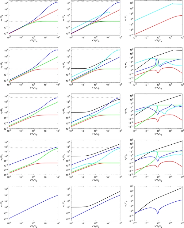
Figure 2. Dispersion and damping curves for parameters appropriate to the VLISM. All parameters are as in Figure 1, including U0 = 200 km s−1 (which ensures that the PUI sound speed Cp is the same), α = 0.999375, but the diffusion is decreased by choosing 〈c2〉1/2 = 50 km s−1. In the left and right panels, the horizontal dotted lines correspond to the asymptotes ω = Ωpcos θ and ω = Ωecos θ. Note that our linear analysis uses exp [i(ωt − k · x)] so that damping corresponds to the positive value of the imaginary part of the frequency. Top panel: θ = 0°, two-fluid wave modes (left); three-fluid with diffusion wave modes showing the real frequency (middle), and the damping rate (right). Second panel: θ = 30°, two-fluid (left); three-fluid real frequency (middle), and damping rate (right). Third panel: θ = 70°, two-fluid (left); three-fluid real frequency (middle), and damping rate (right). Fourth panel: θ = 88°, two-fluid (left); three-fluid real frequency (middle), and damping rate (right). Bottom panel: θ = 90°, two-fluid (left); three-fluid real frequency (middle), and damping rate (right). For the VLISM parameters used here, the modes do not intersect.
Download figure:
Standard image High-resolution imageFigure 2 shows the full complement of the dispersion curves but the level of detail makes it difficult to discern the differences with those curves shown in Figure 1. Illustrated in Figure 3 are the θ = 30° cases for the larger (top panel, 〈c2〉1/2 = 200 km s−1) and smaller (bottom panel, 〈c2〉1/2 = 50 km s−1) diffusion coefficients. The upper panel for the large diffusion example shows that the thermal fast (blue) and slow (red) magnetosonic modes and the Alfvén mode (green) are fundamentally unchanged from the two-fluid waves, and the PUI slow curve (cyan) intersects the thermal fast mode curve. Besides the obvious difference in the PUI fast mode (black curve), the bottom panel shows that (1) the PUI slow mode curve (cyan) no longer intersects the thermal fast mode curve but is "hyperbolic" to it; (2) the PUI slow mode curve completely changes character beyond k ∼ Ωp/VA, and now resembles the thermal fast mode curve in that ωr (and k) increase asymptotically to the electron gyrofrequency Ωecos θ; (3) the thermal fast mode and the Alfvén wave curves approach one another hyperbolically and do not intersect; and (4) the thermal fast mode frequency increases with increasing k, tending asymptotically toward Ωecos θ, but the Alfvén wave (green) curve is now asymptotic to the proton gyrofrequency Ωpcos θ. The behavior of the thermal and Alfvén modes is fundamentally different from the two-fluid model when the PUI heat conduction diffusion coefficient is small enough to ensure coupling of the thermal and PUI plasmas.

Figure 3. Detail of the VLISM θ = 30° cases. The upper panel corresponds to the larger heat conduction diffusion coefficient derived from 〈c2〉1/2 = 200 km s−1, and the lower panel to that derived from 〈c2〉1/2 = 50 km s−1.
Download figure:
Standard image High-resolution imageThe differences between the large and small heat conduction diffusion cases for different obliquities are now readily determined from Figure 2. Observe for example that the PUI slow mode is hyperbolic to the Alfvén mode when θ = 88°.
Consider the high-frequency short wavelength behavior of the two examples shown in Figures 1 and 2. Using the same parameters, we replot the θ = 30° and 88° cases in Figure 4, extending kVA/Ωp to 104. The leftmost column shows the two-fluid dispersion curves, the middle column the three-fluid model where 〈c2〉1/2 = 200 km s−1 is used to estimate the diffusion coefficient (i.e., the Figure 1 case), and the rightmost column illustrates the three-fluid VLISM model using 〈c2〉1/2 = 50 km s−1 (i.e., the Figure 2 case). For the two-fluid plasma model, θ = 30°, notice that the Alfvén mode (green) resonates at the electron cyclotron frequency asymptote Ωecos θ as k → ∞ i.e., at small spatial scales. By contrast, the fast/whistler mode dispersion curve (blue) briefly tracks the electron gyrofrequency Ωecos θ asymptote for a range of wave numbers before eventually continuing to increase with increasing wave number. For highly oblique propagation angles (e.g., θ = 88°), the whistler mode no longer tracks the asymptote Ωecos θ at all and simply continues to increase monotonically.
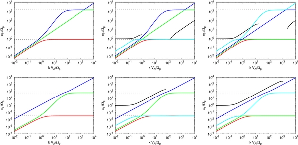
Figure 4. Plots of the real frequencies obtained by solving the three-fluid dispersion relation for the VLISM parameters used in Figures 1 and 2, but now extended to smaller spatial scales (kVA/Ωp < 104). The dispersion relation curves are plotted for propagation angles of θ = 30° and θ = 88°. Top panel: θ = 30°, two-fluid (left), three-fluid with diffusion 〈c2〉1/2 = 200 km s−1 (middle), three-fluid with diffusion 〈c2〉1/2 = 50 km s−1 (right). Bottom panel: θ = 88°, two-fluid (left), three-fluid with diffusion 〈c2〉1/2 = 200 km s−1 (middle), three-fluid with diffusion 〈c2〉1/2 = 50 km s−1 (right).
Download figure:
Standard image High-resolution imageAs discussed above at length, for the large diffusion coefficient case (〈c2〉1/2 = 200 km s−1), the middle panel shows again that the thermal modes in the three-fluid model are not influenced by the PUIs (except for damping) and the three-fluid model behaves as a separate two-fluid and PUI gas. By contrast, the three-fluid model with low PUI diffusion (right panels) exhibits a strong coupling of the thermal and PUI gas, leading to the distinctly different linear wave characteristics discussed in the context of Figures 2 and 3. The small wavelength dispersion curves are similarly different. For θ = 30°, the slow PUI mode curve (cyan) tracks the Ωecos θ line for a range of k values before increasing again with increasing k. The fast thermal mode curve (blue) increases more slowly than the slow PUI mode curve until it approaches the electron gyrofrequency Ωecos θ asymptotically for propagation angles less than the critical angle θc. By contrast, for highly oblique wave propagation angles greater than θc, the slow PUI sound mode (cyan) approaches the electron gyrofrequency Ωecos θ asymptotically and the fast thermal and fast PUI modes now continue to increase beyond the electron gyrofrequency line. Finally, the Alfvén wave dispersion curve, unlike the two-fluid and larger diffusion cases, now approaches the proton gyrofrequency line Ωpcos θ asymptotically rather than the electron gyrofrequency.
Before concluding this section, we further clarify briefly the nature of the interaction of several of the wave modes as revealed in the dispersion relation plots Figures 1, 2, and 3 for oblique propagation. In Figure 5, we consider again the 30° case. The top and bottom panels show the cases illustrated in Figures 1, 2, and 3 for the fast thermal and slow PUI modes. For the 〈c2〉1/2 = 200 km s−1 case, as discussed, the two modes preserve their distinct identities and intersect, i.e., the modes behave as an approximately non-interacting thermal two-fluid and a PUI gas. Reducing the diffusion coefficient by assuming 〈c2〉1/2 = 50 km s−1 (bottom panel) shows that the wave modes no longer preserve their distinct thermal or PUI character—at larger values of wave number k, the thermal fast mode wave behaves more like the PUI slow mode, and the PUI slow mode assumes characteristics of the thermal fast mode. The two modes no longer intersect, as discussed above, as they do in the case of the larger diffusion coefficient. The panels in between illustrate the effect of varying the abundance parameter α (second and third panels down). This variation is somewhat academic since e.g., a value of α = 0.97 requires a VLISM PUI number density of 2.4 × 10⁻³ cm−3, which is unreasonably large for the VLISM, but may be reasonable in other settings. The sensitivity of the wave solutions to the abundance α is revealed in panels 2 and 3 of Figure 5, which show that for a value α = 0.98, the thermal fast and PUI slow dispersion curves intersect, whereas for α = 0.97 they do not. The fourth panel down further illustrates the sensitivity of the dispersion curves to the assumed value of 〈c2〉1/2—in this case 〈c2〉1/2 = 100 km s−1, and the curves resemble the 〈c2〉1/2 = 200 km s−1 example. Figure 5 clarifies that there are two prerequisites for the three-fluid PUI mediated model to behave as a separate thermal two-fluid and PUI charged gas: (1) the PUI number density must be sufficiently low (α must be sufficiently close to (1), and (2) the PUI heat conduction diffusive coefficient must be sufficiently large (large value of 〈c2〉1/2).

Figure 5. θ = 30°, thermal fast mode (blue) and slow PUI (cyan) mode intersections for different PUI abundance and PUI diffusion parameters for the VLISM. The left column of panels show the real frequency as a function of wave number k, and the right column shows the imaginary frequency as a function of k. Note that our linear analysis uses exp [i(ωt − k · x)] so that damping corresponds to the positive value of the imaginary part of the frequency. Top panel: the same parameters as in Figure 1, α = 0.999375 and 〈c2〉1/2 = 200 km s−1; Second panel: α = 0.98 and 〈c2〉1/2 = 200 km s−1; Third panel: α = 0.97 and 〈c2〉1/2 = 200 km s−1; Fourth panel: α = 0.999375 and 〈c2〉1/2 = 100 km s−1; Bottom panel: α = 0.999375 and 〈c2〉1/2 = 50 km s−1.
Download figure:
Standard image High-resolution image4.3. The PUI-mediated Subsonic Solar Wind or the Inner Heliosheath
As discussed in the Introduction, the IHS plasma is mediated in a complex way by PUIs whose origin is both the ISM directly (through charge exchange of interstellar neutrals flowing into the IHS from the local interstellar medium) and PUIs created in the supersonic solar wind and transmitted through the heliospheric termination shock into the IHS. The transmission process is complicated in that some PUIs are transmitted directly and others only after experiencing specular reflection at the shock. The PUI properties inferred theoretically for the IHS as a consequence of these processes (Zank et al. 1996a, 2010; Burrows et al. 2010) have been confirmed and further refined observationally (Richardson 2008; Richardson et al. 2008; Desai et al. 2012, 2014; Zirnstein et al. 2014). The thermal proton density is taken to be ns = 5 × 10⁻³ cm−3 and the ratio of pickup ion to proton density np/ns = 0.2. This yields the parameter α = 1/(1 + np/ns) = 0.833 and the electron density n0 = ns(1 + np/ns) = 6 × 10⁻³ cm−3. The magnetic field is taken to be B0 = 0.1 nT, which yields an Alfvén speed VA = 28.16 km s−1. We assume a proton temperature Ts = 150,000 K, an electron temperature Te = Ts and polytropic indices γs = γe = γp = 5/3. The proton and electron sound speeds are therefore Cs = Ce = 45.43 km s−1. We assume a composite PUI temperature Tp ∼ 107 K, which yields the PUI sound speed classically as  , or Cp = 370.91 km s−1. For the diffusion tensor κ∥ = 〈c2〉/(3Ωp), we assume a characteristic PUI speed of 〈c2〉1/2 = 300 km s−1 and for the perpendicular diffusion coefficient, κ⊥ = χκ∥, we assume χ = 0.01.
Despite the greater mobility of the PUIs in the IHS yielding a larger diffusion coefficient than in the VLISM, the smaller parameter α ensures a strong coupling of the thermal plasma and PUIs. The plots of Figure 6 depicting the real frequency as a function of k therefore resemble those of Figure 2 in many respects. However, for parallel propagation, the two-fluid curves and the thermal modes of the three-fluid model are almost identical. For parallel propagation, the thermal and PUI modes behave as though they are uncoupled (although PUIs damp the thermal modes). The PUI slow mode (cyan) is evanescent for a range of k values, existing for long wavelengths satisfying approximately k ⩽ Ωp/VA and short wavelengths k ⩾ 10Ωp/VA.

Figure 6. Dispersion and damping curves for parameters appropriate to the inner heliosheath or subsonic solar wind. In the left and right panels, the horizontal dotted lines correspond to the asymptotes ω = Ωpcos θ and ω = Ωecos θ. Top panel: θ = 0°, two-fluid wave modes (left); three-fluid with diffusion wave modes showing the real frequency (middle), and the damping rate (right). Only the PUI sound mode (cyan) and the thermal two-fluid sound mode (red) are damped. Over a range of wave numbers, the pickup ion sound mode (cyan) becomes so damped that it loses its identity and disappears (its real frequency becomes zero). All other modes are not damped. Second panel: θ = 30°, two-fluid (left); three-fluid with diffusion, real frequency (middle), and damping rate (right). The PUI fast (black) and slow (cyan) modes no longer cross at small k and both assume characteristics of the other. The PUI slow mode and the thermal fast mode also swap characteristics. Now, the fast PUI mode (black) becomes so damped that it loses its identity and disappears (its real frequency becomes zero) for a range of k before reappearing. Third panel: θ = 70°, two-fluid (left); three-fluid with diffusion, real frequency (middle), and damping rate (right). The fast PUI mode (black) is still so highly damped at small scales that it loses its identity. Fourth panel: θ = 88°, two-fluid (left); three-fluid with diffusion, real frequency (middle), and damping rate (right). Bottom panel: θ = 90°, two-fluid (left); three-fluid with diffusion, real frequency (middle), and damping rate (right).
Download figure:
Standard image High-resolution imageThe dispersion curves change quite dramatically for obliquely propagating modes, and the two-fluid and three-fluid dispersion curves are now quite different. Whereas the parallel PUI slow (cyan) and fast (black) modes intersected, the obliquely propagating modes no longer do so. Instead, as illustrated for θ = 30°, the intersection point becomes "hyperbolic" and the PUI slow and fast modes swap characteristics. Now it is the obliquely propagating PUI fast mode (black) that is evanescent in a range of k space. The PUI slow mode (cyan) becomes quite complicated for oblique propagation, assuming characteristics of not only the PUI fast mode but also the thermal fast magnetoacoustic mode at shorter wavelengths. The PUI slow mode no longer possesses a region that is evanescent.
As illustrated in the two-fluid column of dispersion curves, the behavior of the oblique thermal fast (blue), slow (red) magnetoacoustic and Alfvén (green) modes changes significantly in the presence of PUIs (middle column). For example, both the thermal slow mode and the Alfvén wave tend to the proton gyrofrequency at short wavelengths—the short wavelength behavior of the oblique Alfvén mode is quite different from that exhibited in the two-fluid model.
Finally, the only perpendicularly propagating modes are the PUI and thermal fast modes.
4.4. The PUI-mediated Supersonic Solar Wind Beyond ∼10 AU
The thermal supersonic solar wind beyond the ionization cavity (i.e., >∼10 AU) is dominated by the presence of a suprathermal PUI population comprising primarily protons. Besides protons (Gloeckler et al. 1993), heavier interstellar PUIs are present but in much smaller quantities, first observed in situ by Ulysses (Geiss et al. 1994; Gloeckler et al. 1994) and since by New Horizons (McComas et al. 2008; Randol et al. 2013). We consider solar wind parameters appropriate to 10 AU, assuming that the magnetic field B0 = 0.5 nT, density n0 = 0.08 cm−3, proton temperature Ts = 20,000 K and estimate that the pickup proton abundance is np/ns = 0.05 (5%) so that α = 1/(1 + np/ns) = 0.952. Heavy PUIs are neglected since their number density is extremely small. At ∼10 AU, the Alfvén speed  km s−1. We further assume that the polytropic indices γs = γp = γe = 5/3 and that the electron temperature Te = Ts. The proton and electron sound speeds can be estimated from
  and
and  , which yields Cs = Ce = 16.59 km s−1. We assume a solar wind speed U0 = 400 km s−1, from which we estimate the pickup ion sound speed
  km s−1 under the assumption that the PUI distribution function may be approximated as a filled shell (Vasyliunas & Siscoe 1976; Zank 1999; Zank et al. 2010). The diffusion coefficient is estimated using 〈c2〉1/2 = 400 km s−1.
Plotted in Figure 7, using the same format, as before are the dispersion curves for the two-fluid and three-fluid models for the supersonic solar wind. Consider the top panels first (parallel propagation). The dispersion relation for the three-fluid model is of the 11th-order in ω and generally (at large scales) admits five forward propagating modes, five backward propagating modes and one mode which is purely imaginary. Until now, we have plotted only the five forward modes. Here we plot two additional modes. Starting at large scales (small k), the cyan crosses identify the backward propagating PUI slow sound mode. The real frequency of this mode is negative (and therefore not plotted in the logarithmic scale), but its absolute value is equal to the real frequency of the forward propagating mode (cyan line). The damping rates for the forward (cyan) and backward (cyan crosses) modes are naturally the same, as is illustrated in Figure 7. At kVA/Ωp ∼ 0.7, both the forward and backward PUI slow sound modes become so damped that they lose their identity and become purely imaginary. After this point, the damping rate of these modes is not equal. (Since the modes lost their identity, the decision about which is cyan and which has the cyan crosses is technically ad hoc.) The magenta curve represents the mode that is purely imaginary at large scales. At approximately kVA/Ωp ∼ 18 the damping rates for the magenta mode and the cyan crosses mode become equal. At this point, two new modes with ωr ≠ 0 are generated, one forward (cyan crosses) and one backward (magenta).
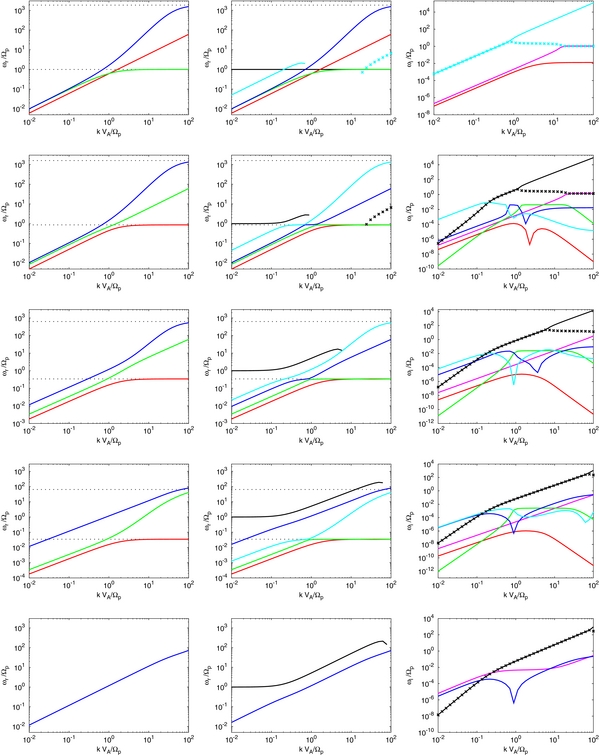
Figure 7. Dispersion and damping curves for parameters appropriate to the supersonic solar wind beyond ∼10 AU. In the left and right panels, the horizontal dotted lines correspond to the asymptotes ω = Ωpcos θ and ω = Ωecos θ. Top panel: θ = 0°, two-fluid wave modes (left); three-fluid with diffusion wave modes showing the real frequency (middle), and the damping rate (right). Second panel: θ = 30°, two-fluid wave modes (left); three-fluid with diffusion wave modes showing the real frequency (middle), and the damping rate (right). Third panel: θ = 70°, two-fluid wave modes (left); three-fluid with diffusion wave modes showing the real frequency (middle), and the damping rate (right). Fourth panel: θ = 88°, two-fluid wave modes (left); three-fluid with diffusion wave modes showing the real frequency (middle), and the damping rate (right). Forward (black line) and backward (black crosses) propagating fast PUI modes lose their identities and become purely imaginary around kVA/Ωp ∼ 60, but no new modes are created at small scales. Bottom panel: θ = 90°, two-fluid wave modes (left); three-fluid with diffusion wave modes showing the real frequency (middle), and the damping rate (right). The PUI fast mode loses its identity at approximately kVA/Ωp ∼ 80.
Download figure:
Standard image High-resolution imageAs shown in the second set of panels (θ = 30°), at approximately kVA/Ωp ∼ 0.9, the fast PUI mode (black) becomes so damped that it loses its identity and becomes purely imaginary. For this reason, we now plot the backward propagating PUI fast mode, represented by black crosses at large scales. After both modes lose their identity at kVA/Ωp ∼ 0.9, their damping rates become unequal and identification of these modes is an ad hoc choice. At approximately kVA/Ωp ∼ 20, the backward propagating PUI (black-crosses) mode matches the frequency of the purely imaginary (magenta) mode. At this point, a new forward propagating PUI fast mode (black crosses) and a new backward propagating mode (magenta line) is generated. The PUI fast (black line) mode now becomes the only purely imaginary mode existing in the system.
Like the θ = 30° case, at 70° the forward (black line) and backward (black crosses) propagating PUI fast modes lose their identities and become purely imaginary at about kVA/Ωp ∼ 6. However, the backward propagating PUI (black crosses) mode never reaches the purely imaginary magenta mode for the k values considered here and no new modes with nonzero real frequency are generated.
5. WAVE MODES IN THE REDUCED ONE-FLUID MODEL
For completeness, we discuss briefly the nature of wave modes admitted by the reduced one-fluid model (61)–(68). The correspondence between these modes and those obtained from the multi-fluid description is noted. The linearization proceeds in the usual way, where we use
and suppose that the fluctuations are ∝exp i[ωt − k · x] and k = (kx, 0, kz). We neglect the higher order PUI viscosity terms and retain only the effects of PUI heat conduction. We obtain the dispersion relation in the form
using the definitions (75)–(76) and  , and θ is the wave propagation angle. The form of (127) is used since it expresses the correspondence with the standard dispersion relation of MHD. By setting k · K · k = 0 (the strong coupling limit) and identifying
  as the sound speed, (127) is identical to the MHD dispersion relation. Alfvén wave propagation is unaffected by PUIs. The expression inside the square bracket of (127) is the dispersion relation for PUI mediated fast and slow magnetosonic modes, by analogy with the multi-fluid analysis.
For wave mode solutions, Equation (127) is usefully expressed as
Before solving (127) numerically, it is useful to introduce κ ≡ κ∥cos 2θ + κ⊥sin 2θ and derive long and short wavelength approximate solutions. We provide the parallel and perpendicular cases first. In the long wavelength limit, we obtain for θ = 0 (parallel propagation)

Equation (129) corresponds to the parallel sound mode propagating at the combined sound speed (i.e., the sum of the square of the thermal plasma sound speed and the PUI sound speed), which is damped by PUIs. Note that in the one-fluid model, the thermal sound and PUI waves are no longer distinct as they were in the multi-fluid model (Equations (94) and (95)). The other parallel mode admitted by (130) is unaffected by PUIs, and corresponds to the Alfvén wave solution obtained from the first bracketed term of (127). Finally, Equation (131) describes a purely imaginary non-propagating mode. For perpendicular propagation, θ = π/2, the long wavelength limits become
The fast mode speed now includes the Alfvén speed, in accordance with MHD, as well as the PUI sound speed, and is damped by PUIs. The slow mode is non-propagating and purely damped. The comments regarding the comparison to the multi-fluid modes above hold for perpendicular propagation as well.
The short wavelength limits of (128) for parallel propagation are

and for θ = π/2,


The PUIs no longer contribute to the fast mode sound speed, as they did in the long wavelength regime, but the PUIs do damp the thermal plasma fast mode. The slow mode in the short wavelength limit is completely unaffected by the presence of PUIs.
Consider now the general case of oblique wave propagation. For all angles of propagation, we always have the classical Alfvén wave solution

which is completely unaffected by the presence of a suprathermal PUI population. The obliquely propagating long wavelength mode is somewhat complicated, with

where
The purely imaginary mode in the long wavelength limit is
For short wavelength modes propagating obliquely, we have the general result
The real frequency is unaffected by PUIs and is identical to the familiar MHD fast and slow magnetosonic speeds. Damping of the short wavelength fast and slow modes is directly due to PUIs, however. The parallel and perpendicular limits are consistent with our previous results.
The purely imaginary non-propagating short wavelength mode is given by
For parallel and perpendicular propagation, we have
Numerical solutions of the dispersion relation (127) are plotted in Figure 8 for VLISM parameters. The heat conduction diffusion coefficient was estimated assuming 〈c2〉1/2 = 200 km s−1. The left column shows the real frequency plotted as a function of k and the right column shows the corresponding imaginary frequency. We do not plot the purely imaginary mode. Only three real modes exist—the fast (blue) and slow (red) magnetosonic modes modified by PUIs, and the Alfvén wave (green). For parallel propagation, the slow mode coincides with the Alfvén mode, and there is a region around k ≃ Ωp/VA for which the fast mode is evanescent. For quasi-parallel propagation (e.g., θ ⩽ 30°), the region of evanescence for the fast mode is always present, but for quasi-perpendicular propagation (e.g., third panel of Figure 8), the fast mode exists for all wave numbers k. For the VLISM parameters used here, the slow mode and Alfvén wave are virtually indistinguishable, although the former is damped by PUIs.
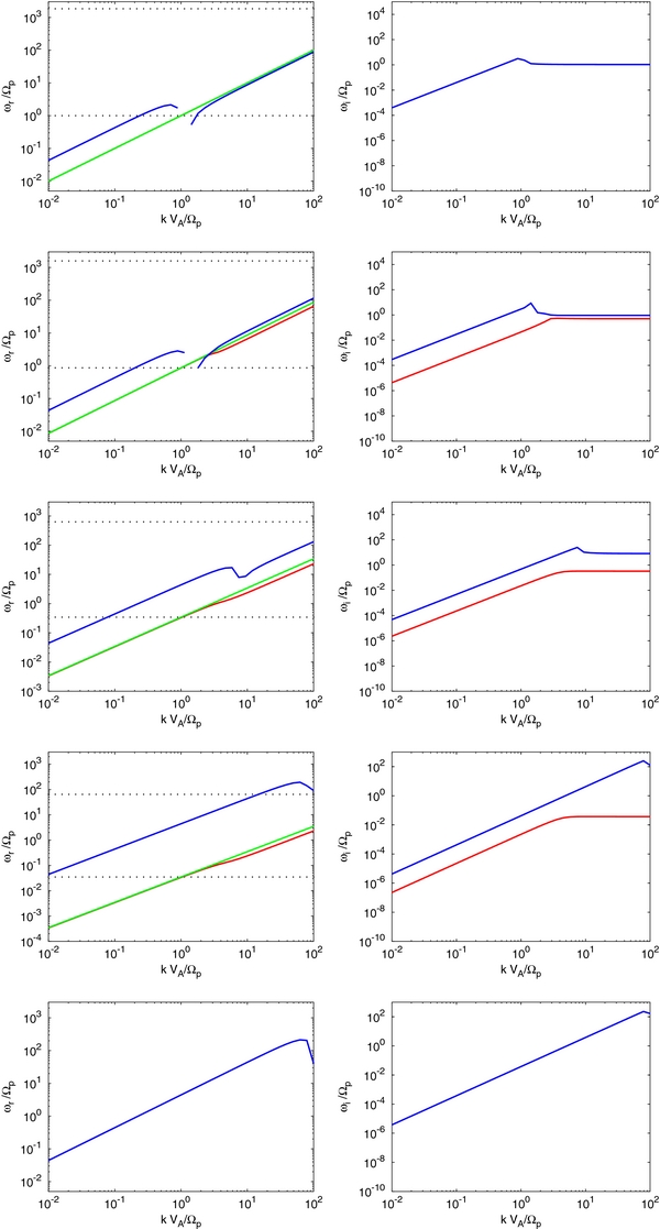
Figure 8. Dispersion and damping curves for the one-fluid model mediated by PUIs, for VLISM parameters and α = 0.999375 and 〈c2〉1/2 = 200 km s−1. The left column shows plots of the real frequency as a function of wave number k, and the right column shows the corresponding imaginary frequency. The fast mode is shown by the blue curve, the slow mode by red, and the Alfvén wave by green. Top panel: θ = 0°. Second panel: θ = 30°. Third panel: θ = 70°. Fourth panel: θ = 88°. Bottom panel: θ = 90°.
Download figure:
Standard image High-resolution image6. SUMMARY AND DISCUSSION
Pickup ions typically dominate the internal energy and do not equilibrate collisionally in plasma systems such as the VLISM, the IHS, and the supersonic solar wind beyond some 10 AU. This requires that we treat PUIs as a distinct plasma component. PUIs experience pitch-angle scattering from pre-existing and self-excited magnetic field turbulence. We have developed a collisionless form of Chapman–Enskog expansion that is correct to second order to effect the closure of the moments of the PUI transport equation. The first-order expansion of the PUI distribution function introduces the collisionless PUI heat flux through a heat conduction diffusion tensor. We show that the collisionless PUI heat conduction term is proportional to the gradient in the PUI pressure. The second-order expansion of the PUI distribution function yields the collisionless stress tensor for PUIs, whose structure generalizes the familiar form from hydrodynamics (e.g., Zank 2013). By deriving expressions for the PUI heat flux and stress tensor in terms of lower order moments (PUI pressure and bulk velocity) we can derive a closed form of multi-fluid equations for a plasma system comprised of thermal protons and electrons and suprathermal PUIs. The system of equations differs from the typical multi-fluid system in that we have made no ad hoc assumptions about the PUI distribution being isotropic but instead derived the heat flux and stress tensor corrections subject to weak departures from isotropy (i.e., assuming that the scattering of PUIs by turbulent magnetic fluctuations proceeds rapidly).
Since many problems are too complicated to solve using an elaborate multi-fluid model, we develop an analogue to the MHD equations that resembles a single-fluid description but possesses a separate equation of state for the PUIs, together with a separate equation of state for the thermal background plasma. In so doing, the single-fluid description now includes both collisionless heat conduction and stress tensor (collisionless viscosity) tensor terms associated with the PUIs. The derived single-fluid model possesses an interesting structural similarity with the so-called cosmic ray MHD model (Webb 1983). The single-fluid PUI-mediated MHD equations presented here are almost identical to the cosmic ray (CR) MHD equations but the derivation is entirely different. The derivation of the CR MHD equations explicitly neglects all the flow acceleration and shear terms (which, as we have shown above, is essential in the derivation of the closed fluid system describing the pitch-angle scattered charged particles), does not derive the underlying multi-fluid description from which an MHD description is developed, explicitly assumes that the cosmic ray proton number density is zero, and assumes an ad hoc decomposition of the total isotropic scalar pressure into thermal and cosmic ray components. Of particular interest is that the PUI number density is included in the PUI-mediated single-fluid equations, suggesting that a more careful corresponding derivation of the CR MHD equations could also lead to the explicit inclusion of the CR number density. The importance of this is that it allows the "injection" problem for the acceleration of cosmic rays at collisionless shocks to be addressed within the context of the single-fluid CR MHD equations (e.g., Zank et al. 1993).
We have used our new PUI-mediated plasma model to investigate the nature of linear waves in the context of the VLISM, the IHS or the subsonic solar wind, and the supersonic solar wind beyond ∼10 AU using the full multi-fluid description. The general dispersion relation in the presence of PUIs and a background thermal plasma comprised of protons and electrons was derived—this includes the effects of the collisionless heat conduction (diffusive) term, but we neglect the effects of the (viscous) stress tensor terms. The retention of the electron inertia terms yields a formidably complicated dispersion relation that does not lend itself to analytic representation. Consequently, the fully general dispersion relation is solved numerically only. Prior to solving the full dispersion relation (i.e., with electrons, thermal protons, and PUIs retained), we derive an analytically "tractable" dispersion relation under the assumption of massless electrons. An 11th-order polynomial dispersion relation is obtained in the low-frequency (ω ≪ Ωe) limit, which we investigate analytically for a variety of cases. The class of admissible wave solutions is of course richer than in the standard two-fluid case, with as many as five distinct propagating (real frequency) wave modes are possible: forward and backward propagating Alfvén waves, thermal fast and slow magnetoacoustic waves, and PUI fast and slow magnetoacoustic waves, as well as an entropy mode. At least one purely damped, non-propagating mode also exists. The thermal wave modes are characterized by their real frequency being proportional to the thermal sound speed  to leading order, whereas the PUI modes are proportional to the PUI sound speed Cp to leading order. However, all the waves are damped by PUIs, whether thermal or PUI modes. These results were obtained from an analytic expansion of the 11th-order dispersion relation in the short and long wavelength limits for parallel, perpendicular, and oblique wave propagation. The analysis shows that the damping of both the long and short wavelength waves is a direct consequence of the collisionless PUI heat conduction, i.e., diffusive damping. In the short wavelength limit, we find that the PUI modes are absent, with only the thermal modes and a mixed mode existing.
The analytic limits are interesting and provide useful insight and guidance in understanding and classifying the numerical solutions that are necessary to understand the full complexity of the dispersion relations when electron inertial terms are retained. In solving the linearized full multi-fluid system numerically, we also examine the reduced two-fluid solutions that emerge from the abundance limit α = 1. In the α = 1 limit, the full dispersion relation separates into separate two-fluid and PUI fluid dispersion relations. The two-fluid dispersion relation is the familiar sixth-order polynomial relation first investigated by Stringer (1963; we have corrected a number of simplifications and typos that were present in earlier derivations of the two-fluid dispersion relation). Solutions of the two-fluid dispersion relation are useful in clarifying the numerical solutions when α < 1, and in showing explicitly the role that PUIs play in mediating wave properties. We considered parameter regimes for three distinct plasma environments that are mediated by PUIs created in part by interstellar neutral H.
A major application of the linear wave theory was to the plasma of the VLISM. As discussed, the IBEX observations appear to confirm the notion that the VLISM is comprised of a non-equilibrated admixture of thermal plasma and energetic PUIs created by fast neutrals originating in the supersonic and hot subsonic (IHS) solar wind (Zirnstein et al. 2014; Desai et al. 2014). The VLISM parameters can be reasonably estimated, including the abundance parameter α (Zirnstein et al. 2014), but the choice of value for the collisionless heat conduction term is less well constrained in the context of the multi-fluid model. Two estimates of the diffusion coefficient K were considered, one corresponding to the weak coupling of PUIs to the thermal plasma (i.e., a large value of the diffusion coefficient for the collisionless PUI heat flux) and the other to a slightly stronger coupling. Both values of the diffusion coefficient appear to be reasonable but the results for the two cases differ quite significantly. Both cases can yield as many as five distinct wave modes (depending on the wave number k). We find the following.
- 1.For κ∥ large, the thermal and PUI modes are essentially decoupled from one another in that the dispersion curves (the real frequency as a function of k) of the thermal modes (fast, slow, and Alfvén) very closely resemble those obtained from the two-fluid model (i.e., in the absence of PUIs). The fast and slow PUI modes are present and the thermal and PUI dispersion curves can intersect but there is no corresponding modification to either mode in the regions of intersection in (ω, k) space.
- 2.Even when the diffusion coefficient is large and the thermal and PUI fluid essentially decouple, the PUIs nevertheless act to damp both the thermal and PUI modes, and the Alfvén mode (illustrated in the plots of the imaginary frequency as a function of k).
- 3.The interplay between the fast and slow PUI modes is interesting for the larger choice of diffusion coefficient. For parallel wave propagation, the slow PUI wave is evanescent above a certain wave number and the fast PUI mode is undamped and satisfies ω = Ωp. However, for oblique wave propagation, the fast mode is evanescent at short wavelength scales and the slow PUI wave is asymptotic to Ωpcos θ at short wavelengths.
- 4.For κ∥ smaller, the PUI and the thermal modes are fully coupled and the two-fluid results are no longer a useful guide to the oblique wave properties in either the long or short wavelength regimes, particularly for wave numbers approximately >Ωp/VA. Only for parallel propagation do the thermal wave mode dispersion curves resemble the two-fluid dispersion relations.
- 5.For smaller κ∥, the various dispersion curves no longer intersect as they do for a larger diffusion coefficient. Instead, the dispersion curves in the vicinity of an apparent intersection point are modified in that they approach one another in a "hyperbolic" sense but do not cross. Furthermore, the properties of the converging dispersion curves "exchange properties" in these regions. For example, the dispersion curve for the slow PUI mode resembles what was the parallel thermal fast mode curve at short wavelengths.
- 6.Of possible particular importance is that the dispersion curve for Alfvén waves completely changes character from the large diffusion coefficient case to the smaller diffusion case. In the former example, the Alfvén wave dispersion curve is asymptotic to Ωecos θ and in the latter to Ωpcos θ.
We do not summarize the detailed properties of the linear wave analysis applied to the IHS or subsonic solar wind. The wave properties resemble the smaller diffusion coefficient VLISM case despite the nominal diffusion coefficient being larger in the IHS than in the VLISM. This is because the abundance parameter α is smaller than it is in the VLISM, so ensuring a stronger coupling of thermal and PUI plasma. Similarly, our analysis of the linear wave modes in the supersonic solar wind beyond ∼10 AU revealed that the wave properties were similar to those of the small diffusion coefficient VLISM example. As part of the supersonic solar wind analysis, we considered the backward propagating PUI modes as well, showing how fast forward and backward propagating PUI modes could lose their identity and become purely evanescent or imaginary. Correspondingly, when a backward propagating PUI mode matches the frequency of an imaginary PUI mode, then new forward and backward propagating modes are generated.
For completeness, we considered linear wave solutions of the reduced one-fluid PUI-mediated plasma model. Because the reduction to a single plasma with equations of state for both constituents (thermal plasma and PUIs) eliminates the distinction between the plasma components, the distinction between PUI and thermal wave modes is lost.
- 1.The single-fluid or one-fluid model only admits three propagating waves—the fast mode, slow mode, Alfvén mode, and a purely imaginary mode.
- 2.Long wavelength modes propagate at a mixed fast or slow magnetoacoustic speed where the sound speed is now a combination of the thermal sound speed and the PUI sound speed, i.e.,
 .
. - 3.Short wavelength modes propagate at the fast or slow magnetosonic speed where the sound speed is given by the thermal sound speed only, i.e., PUIs do not contribute to the phase velocity of short wavelength waves.
- 4.Both fast and slow mode, obliquely propagating modes are damped by the heat flux term associated with PUIs. For parallel propagation in both the long and short wavelength limits, the slow mode wave is identical to the Alfvén wave, and is undamped. This does not hold for oblique wave propagation.
- 5.Unlike the multi-fluid model, Alfvén waves in the one-fluid reduced model are unaffected by PUIs and the dispersion curve continues to increase with increasing k, as in the case of ideal MHD.

The compressibility and polarization of the various waves was not discussed here. Furthermore, we note that the inclusion of Landau damping can modify the multi-fluid description in important ways, as described in Hunana et al. (2013).
One important implication to emerge from our three-fluid analysis of linear waves is related to the contrasting behavior of the two-fluid waves, particularly the Alfvén mode in the case of strong PUI and thermal plasma coupling. Our results suggest that turbulent fluctuations in the inner heliosphere may be fundamentally different from those in regions such as the supersonic solar wind beyond ∼10 AU, the IHS, or the VLISM. Precisely how this translates into e.g., observed magnetic field fluctuation spectra is an open question, but we note that Burlaga et al. (2006); Burlaga & Ness (2009) have observed "turbulence" in the IHS that appears to possess characteristics (distribution, compressibility) somewhat different from those observed in the inner heliosphere (e.g., Bruno & Carbone 2005). Initial observations of the VLISM by the Voyager 1 magnetometer (Burlaga & Ness 2014) suggest a surprisingly low level of magnetic field fluctuations. In the absence of significant external driving, it is possible, based on the results presented here, that PUIs act to damp waves in the VLISM significantly, leaving the medium relatively quiescent.
A second important implication is related to heavy ions that are minor components in the solar wind of the inner heliosphere and in cometary environments. Mann et al. (1997) used a three-fluid system of fluid equations to derive the dispersion relation for a proton–electron-heavy ion plasma and investigated the wave properties based on this model. However, the model is closed by assuming Maxwellian distributions for all the species. In both a cometary environment and in the inner heliosphere, heavy ions experience pitch-angle scattering off ambient and excited turbulent magnetic fluctuations and are not equilibrated with the background thermal plasma. In view of the important differences that we have identified in the dispersion curves as a consequence of deriving and including the collisionless heat flux associated with PUIs (and in principle the collisionless stress tensor) into a multi-fluid model, we suspect that that similar differences might well arise from extending our approach to heavy ions.
In subsequent papers, we plan to examine further the damping of waves in PUI mediated plasmas, including heavy ions, explore nonlinear waves and structures admitted by this system, and investigate the structure of shock waves in the presence of PUIs.
Finally, we note that the PUI mediated plasma model presented here can find application to a wide variety of astrophysical situations, ranging from the interaction of solar-like stars with different interstellar conditions (e.g., Müller et al. 2006; Florinski et al. 2004) to the propagation of shock waves in a partially ionized ISM (e.g., Raymond et al. 2008).
This work was supported by IBEX NASA/SwRI award NNG05EC85C, subcontract A99132BT and NASA grant NNX10AC17G. G.P.Z. appreciates discussions at the team meeting "Heliosheath Processes and Structure of the Heliopause: Modeling Energetic Particles, Cosmic Rays, and Magnetic Fields" supported by the International Space Science Institute in Bern, Switzerland.
APPENDIX A: TRANSPORT EQUATIONS FOR PUIS
The gyrophase-averaged equation for non-relativistic particles is given by
where the direction vector b ≡ B/B. We use a Legendre polynomial expansion to solve the gyrophase-averaged equation (A1), expanding the gyrophase-averaged particle distribution function f as

Following the derivation in Zank (2013), we obtain an infinite set of partial differential equations in the coefficients fn of the Legendre polynomials,
For the f2 approximation (i.e., assume fn = 0 ∀ n ⩾ 3), we have, on setting m = 0,

and on setting m = 1 and neglecting all terms with indices having i ⩾ 3, we obtain
where the f0 Legendre coefficients are expressed as source terms in the evaluation of the next order Legendre coefficients f1. To solve Equation (A4) for f1 in terms of the lower order Legendre coefficient f0, we assume that the zeroth-order coefficient f0 is almost isotropic, implying that f1 ≪ f0. We also assume that  is large, i.e., rapid scattering of the charged particles (which is consistent with the assumption that the particle distribution is nearly isotropic), so that the term νsf1 ∼ O(f0). Subject to these assumptions, Equation (A4) can then be solved, yielding

Using (A5) in (A3) to rewrite f1 in terms of f0 yields the familiar transport equation in the presence of large-scale gradients and accelerations (see Zank 2013) if the f2 terms are neglected,

where K is the diffusion tensor.
The m = 2 expression can be written as
from which we obtain the approximate solution for f2,

APPENDIX B: THE DISPERSION RELATION WITHOUT ELECTRON INERTIA


Footnotes
- 4
We note that the classical two fluid dispersion (Stringer 1963; Formisano & Kennel 1969; Braginskii 1957)—sometimes called the low-frequency dispersion relation since the displacement current is neglected and high-frequency modes are eliminated—employs a slightly simplified derivation that combines the proton and electron momentum equations and neglects some terms proportional to ξ (see, e.g., Appendix I in Stringer 1963). These classical forms of the dispersion relation are therefore not completely equivalent to (115)–(116), which is the exact two-fluid dispersion relation with no displacement current. For numerical solutions the differences are however negligible. We also note that the otherwise exact two-fluid dispersion of Sahraoui et al. (2012; their Equation (13)) contains a small typo in the first term in front of ω6 (our A6 term), which in our case expands as
. Instead of the correct (1 + ξ)2 Sahraoui et al. have 1 + ξ2 (however, for their numerical solutions F. Sahraoui et al. 2014, private communication, used the correct dispersion relation).
![$(1+\xi)[ (1+\xi)^2 +2\xi (1+\xi)({k^2 V_A^2}/{\Omega _p^2})+\xi ^2({k^4 V_A^4}/{\Omega _p^4})]$](https://content.cld.iop.org/journals/0004-637X/797/2/87/revision1/apj503996ieqn21.gif)