


ABSTRACT
We have developed a procedure for observing and tracking proper motions of faint XUV coronal intensity on the Sun and have applied this procedure to study the collective motions of cellular plumes and the shorter-period waves in sunspots. Our space/time maps of cellular plumes show a series of tracks with the same 5–8 minute repetition times and ∼100 km s−1 sky-plane speeds found previously in active-region fans and in coronal hole plumes. By synchronizing movies and space/time maps, we find that the tracks are produced by elongated ejections from the unipolar flux concentrations at the bases of the cellular plumes and that the phases of these ejections are uncorrelated from cell to cell. Thus, the large-scale motion is not a continuous flow, but is more like a system of independent conveyor belts all moving in the same direction along the magnetic field. In contrast, the proper motions in sunspots are clearly waves resulting from periodic disturbances in the sunspot umbras. The periods are ∼2.6 minutes, but the sky-plane speeds and wavelengths depend on the heights of the waves above the sunspot. In the chromosphere, the waves decelerate from 35–45 km s−1 in the umbra to 7–8 km s−1 toward the outer edge of the penumbra, but in the corona, the waves accelerate to ∼60–100 km s−1. Because chromospheric and coronal tracks originate from the same space/time locations, the coronal waves must emerge from the same umbral flashes that produce the chromospheric waves.
Export citation and abstract BibTeX RIS
1. INTRODUCTION
Time-lapse movies of 193 Å coronal images, obtained with the Atmospheric Imaging Assembly (AIA) on the Solar Dynamics Observatory (SDO) spacecraft (Lemen et al. 2012) and enhanced to indicate the proper motions of faint coronal intensity (Stenborg et al. 2011), give the appearance of large-scale flows moving across the disk of the Sun. The flow moves from head to tail along the cellular plumes seen in 193 Å images (Sheeley & Warren 2012; Sheeley et al. 2013) and resembles the large-scale pattern of chromospheric fibrils seen in Hα images (Foukal 1971; Sheeley 1981). Like the cellular plumes, the proper motions are directed along magnetic fields that originate in one pole of a bipolar magnetic region and extend horizontally outward across a unipolar magnetic region until they encounter a distant filament channel and are deflected sideways. Also like the plumes, the flow moves in the opposite direction on the other side of the filament channel, giving the impression of a divided highway of oppositely directed motion extending to great distances across the Sun.
Our original objective was to use AIA images to study this large-scale motion as an application of our newly developed procedure for observing and tracking proper motions of extreme ultraviolet (XUV) coronal intensity. As shown in Section 3, the procedure quickly revealed that the apparent large-scale flows are the collective effect of independent and repeated ejections from the unipolar flux concentrations at the bases of the plumes. It became obvious that the apparent large-scale motion was more like a system of independent conveyor belts aligned end to end than a continuous flow across the Sun. In addition, we discovered that the properties of these ejections were similar to those found previously in coronal fans at the ends of active regions (De Moortel 2005; Stenborg et al. 2011; Tian et al. 2011b; De Moortel & Nakariakov 2012; Wang et al. 2013a) and in the plumes that occur in coronal holes both at the Sun's poles and at lower latitudes (Deforest & Gurman 1998; McIntosh et al. 2010; Tian et al. 2011a; Krishna Prasad et al. 2011). Thus, aside from the improved tracking procedure, our main contribution is to emphasize the global character of the apparent flow and the widespread nature of the cellular plumes that are its defining components.
However, in the process of tracking the motions within cellular plumes, we discovered that this observing and tracking procedure is an ideal way of studying the shorter-period waves that occur inside sunspots (De Moortel et al. 2002; Jess et al. 2012; Reznikova & Shibasaki 2012; de la Cruz Rodríguez et al. 2013), especially when the lag used with the difference images is adjusted to match the 1.3 minute half period of these waves. In this case, the sunspot disturbances are highly periodic and spread out in clear, concentric wavefronts. By comparison, the disturbances in cellular plumes are often linear features stretching along the local field direction and repeating after times in the relatively broad range of five to eight minutes. Thus, if these disturbances in cellular plumes are waves, they are quite different than sunspot waves.
Meanwhile, recent improvements in software at the Lockheed/Stanford Joint Science Operations Center (JSOC), made it possible for us to download and process comprehensive observations of several sunspots in a variety of situations including their emergence, their disk transit, and their location at the extreme limb—far more material than we are able to reproduce here. Instead, in this paper, we provide a sample of these new observations, summarizing our current understanding of the waves and comparing them with our measurements of the motions in cellular plumes. We leave a discussion of the more complete set of observations to a later paper.
We do this in the following way. In Section 2, we give a detailed account of the new measurement procedure. Then in Section 3, we use this procedure to measure the motions in cellular plumes and in sunspots. In Section 4, we summarize and discuss these results; and in Section 5, we conclude with the overall impression that we gained from this work. In Appendix A, we calculate the lagged differences that might be expected for a variety of input waves, and derive the important result that the difference signal is proportional to ![$\sin [({\pi }/2)({\Delta }t/{\tau ^{^{\prime }}})]$](https://content.cld.iop.org/journals/0004-637X/797/2/131/revision1/apj504485ieqn1.gif) , where Δt is the lag time and
, where Δt is the lag time and  is one-half of the oscillation period. In Appendix B, we derive the current-free field of an idealized magnetic monopole located in a uniform horizontal magnetic field, as a way of simulating the structure that we observe in AIA 193 Å images of unipolar magnetic regions. (As we discussed previously (Sheeley & Warren 2012), the cellular plumes have temperatures ∼1.2 MK, and therefore are not well visible in Å 171 Å images, except in coronal holes and in the bright fans at the ends of active regions.) Finally, in Appendix C, we compare the frequency spectra of the repeated motions in cellular plumes and in the sunspot waves.
2. MEASUREMENT PROCEDURE
Our data source consists mainly of observations obtained with the AIA instruments on the SDO spacecraft (Lemen et al. 2012), as mentioned above. The AIA observations are full-disk (∼1.2 R☉) images obtained in 10 wavelength bands: Fe xviii 94 Å, Fe xx 131 Å, Fe ix/x 171 Å, Fe xii 193 Å, Fe xiv 211 Å, He ii 304 Å, Fe xvi 335 Å, C iv 1600 Å continuum, 1700 Å continuum, and 4500 Å continuum. The spatial resolution was about 0 6. The cadence was 12 s for the seven coronal lines, 24 s for the ultraviolet continuum images, and 1 hr for the 4500 Å continuum images. However, as discussed below, for our purposes, the images fell into essentially three distinct classes represented by Fe ix/x 171 Å, which showed active region fans and other spiky structures; Fe xii 193 Å, which showed coronal plumes; and He ii Å, which showed chromospheric features. After some initial comparison and experimentation, we concentrated on images obtained in these three passbands. We supplemented these XUV observations with 6173 Å magnetograms (to show the associated photospheric fields) and continuum images (to show sunspots). These data were obtained with the Helioseismic Magnetic Imager (HMI; Scherrer et al. 2012), also on the SDO spacecraft. These images were obtained with a spatial resolution of about 05 and a temporal cadence of 45 s.
We have previously used running difference movies to study the motion of material through the outer corona (Sheeley et al. 1997, 1999). For sufficiently slow speeds, the difference signal was equal to the product of the speed, the time lag, and the intensity gradient of the feature being tracked. Thus, our only constraint was to select a lag that was large enough to give an appreciable signal in the movies. For most streamer blobs and slow coronal mass ejections, this lag was about 20 minutes. In the outer corona, the motions tended to be radially outward along streamers, which allowed us to use a straight slit to construct the space/time maps. We referred to these maps as "jmaps", and, for simplicity, we will continue to use this term in the remainder of this paper.
There are several differences between the proper motions along streamers in the off-limb white-light corona and the proper motions along the plumelike structures in the on-disk Fe xii corona. First, the on-disk motions are not usually directed along straight paths, but instead occur along the curved plumes that seem to outline the direction of the magnetic field. We solved this problem by extracting the difference intensity in small, linear segments along the curved path and then rearranging those segments end-to-end to produce a rectangular display. This approach is analogous to using small, linear rulers to measure distance along a curved path. In principle, this segmented approach is not as smooth as the spline-fit approaches (see Stenborg et al. 2011 and references contained therein), but the difference is small when the segments are kept short compared to the curvature of the path. In addition, the segmented approach allows paths with discontinuous changes in slope, which we found useful for generating symmetric, chevron patterns of tracks from paths that switched back nearly upon themselves.
A more difficult problem was that unlike the motions in the outer corona, the Fe xii motions close to the Sun are periodic, or at least repetitive (De Moortel 2005; McIntosh et al. 2010; Stenborg et al. 2011; Tian et al. 2011b; De Moortel & Nakariakov 2012; Jess et al. 2012; McIntosh et al. 2012; Wang et al. 2013a). Thus, we might expect the visibility of these motions to be affected by the lag used in the running difference images. For example, a lag of 5 minutes ought to weaken motions with a 5 minute period by subtracting them in phase, whereas a lag of 2.5 minutes would strengthen these motions by subtracting them 180° out of phase. In fact, as described in Appendix A, the difference signal ought to be proportional to ![$\sin [({\pi }/2)({\Delta }t/{\tau ^{^{\prime }}})]$](https://content.cld.iop.org/journals/0004-637X/797/2/131/revision1/apj504485ieqn3.gif) , where Δt is the lag and
, where Δt is the lag and  is one-half of the oscillation period. In practice, we found a tendency toward this result, especially for the sunspot waves, which produce a strongly periodic signal. However, we were never able to null out the oscillations entirely for any choice of lag, probably due to several factors, including spectral impurity, amplitude variations, and our discrete choices of the lag. Thus, as described below, we settled on an effective lag of 144 s to study the 5–8 minute cellular plumes and an effective lag of 72 s to study the 2.6 minute oscillations in sunspots.
Also, unlike the white-light observations of the outer corona, the Fe xii 193 Å observations depend on the temperature of the coronal plasma. If the thermal lifetime of the plasma is short compared to the transit time of the motion, then it will be difficult to obtain meaningful tracks of the motion. Thus, short lifetimes of active-region loops may account for why we have not succeeded in obtaining high quality jmaps of their motions. Conversely, our success tracking disturbances along the plumes in unipolar magnetic regions suggests that the lifetimes of those disturbances are at least comparable to their transit times along the plumes. Of course, there is always the question of what lines are contributing to the bandpass of interest (O'Dwyer et al. 2010), and, as described below, it is possible that some of the decelerating waves found in coronal observations of sunspots result from contributions of weak lines formed close to the Sun. However, in general, we will refer to each spectral bandpass of the AIA instrument in terms of its dominant contributors (i.e., Fe xii 193 Å, Fe ix 171 Å, and He ii 304 Å), realizing implicitly that other weak lines in the respective bandpasses might be contaminating some of the observations.
Although the propagating disturbances occur in unipolar regions throughout the Sun, their intensity variations are small (≲5% of the background intensity) and difficult to see in unprocessed time-lapse movies. Consequently, we began with a 60 minute sample of 300 images obtained with a 12 s cadence, and considered various ways of averaging them to reduce the noise. We decided on a three-frame average, which changed the temporal resolution to 36 s and decreased the number of frames to 100. Next, we experimented with the time lag for making difference images of these 100 frames, and settled on a 4 frame lag, corresponding to 144 s or approximately half the dominant 5 minute period of the photospheric oscillations. This lag provided a compromise between spatial resolution (which decreased with lag) and signal strength (which increased), and is adequate for detecting motions with periods in the range 5–10 minutes. Because this lag slightly reduced the strength of oscillations with periods in the 2–3 minute range, we reduced the lag to two frames (72 s) to study the 2.6 minute sunspot waves, but retained the three-frame average in order to see the faint chromospheric component of these waves. (We obtained slightly better spatial resolution with an equivalent three-frame lag of two-frame averages, but at the expense of reduced sensitivity.) Finally, we corrected the maps for solar rotation (so that the movies panned with the solar region of interest), and then we used these lagged difference movies to construct jmaps of the observed proper motions.
To track the proper motions, we modified the software that we had developed for studying time-lapse movies obtained with the Transition Region and Coronal Explorer spacecraft (Sheeley et al. 2004). In our new version of this software, we displayed the movie frames (either subtracted or unsubtracted) in one panel of the computer screen and the jmap in an adjacent panel. To follow the motion along a curved path in the movie, we marked off a sequence of points along that path by clicking along it with a mouse. We saved these points for later use with other movies that we might construct for this same region of the Sun. The program connected the adjacent points to form line segments along the curved path. Next, we expanded the individual line segments laterally to form mini-slits of the desired width. After filling these mini-slits with the intensity difference from each movie frame, we rotated the slits into the north-south direction and placed them end-to-end to form a continuous, rectified strip. Then, we stacked these strips chronologically to give a rectangular jmap of intensity difference as a function of time (on the horizontal axis) and distance (on the vertical axis). Once we defined the sequence of points, it took only a few seconds to create the jmap for a 100 frame movie.
A useful capability of the software was the ability to toggle back and forth between a distance–time location on the finished jmap and the corresponding location along the path in the movie image. This allowed us to identify the features that produced the tracks and vice versa. Also, because the individual points were saved, the path could be reconstructed and used to make jmaps with different spectral lines (like Fe ix 171 Å or He ii 304 Å) or different choices of slit width, time lag, or frame averaging for the same spectrum line.
In the initial application of this procedure, we downloaded full-resolution coronal images and magnetograms of regions near the central meridian for 43 days during the interval 2011–2013 and used these observations to make space/time maps for various combinations of paths, slit widths, and time lags. More recently, we have included regions at other positions on the solar disk and above the limb and have begun to use center-to-limb variations to probe the three-dimensional structure of the sunspot waves. In the next section, we provide examples of these jmaps together with individual "slit-jaw" images showing the paths used in the construction of these jmaps.
Finally, we note that an important aspect of a jmap is to provide speeds of the features being tracked. These speeds are determined by measuring the slopes of the height/time tracks and refer to the sky-plane component of motion. In general, this sky-plane component will differ from the true speed by an amount that depends on the orientation of the feature being tracked and its center-to-limb position on the solar disk. For a sunspot wave in the chromosphere, the sky-plane speed may be approximately equal to the true speed if the sunspot is near the disk center, but for coronal motions, a correction may be necessary. In this paper, we have not attempted to correct for this effect, so our measured speeds refer to sky-plane values unless otherwise indicated.
3. OBSERVATIONS
3.1. Tracking Motions along Single and Multiple Plumes
Figure 1 compares an AIA Fe xii 193 Å image with an HMI line-of-sight magnetogram of a unipolar magnetic region near disk center on 2012 July 30. Concentrations of positive-polarity (white) flux are interspersed with barely visible specks of negative-polarity (black) flux, and a number of cellular plumes are associated with these elements of positive polarity. The co-aligned arrows point to one of these flux concentrations and to the corresponding coronal position from which diverging motions were visible in the running difference image movie. This position lies about 20 Mm (roughly half the 40 Mm length scale of the arrows) from the nose of the plume, not at the nose itself where another bright knot and small bipolar magnetic region are located.
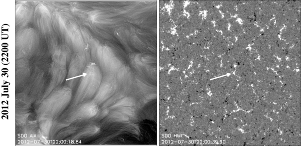
Figure 1. Comparison of an AIA 193 Å Fe xii image (left) and a nearly simultaneous HMI 6173 Å magnetogram (right), showing cellular plumes rooted in photospheric concentrations of positive-polarity (white) magnetic flux. Co-aligned arrows (of approximately 40 Mm length) point to the magnetic flux element and to the corresponding source of coronal ejections shown in the next two figures.
Download figure:
Standard image High-resolution imageThe top panel of Figure 2 zooms in on this cellular plume, showing the path used to create a space/time map (henceforth jmap) of proper motions along the plume. The path is indicated by three closely spaced dashed lines (yellow in the online version). A central line connects the points (faint plus signs) that define the path. This central line is flanked by two additional lines whose separation indicates the (∼3.0 Mm) width of the slit used to construct the jmap. The resulting path runs southward (downward) from the place that we observed diverging motions in the corresponding running difference image movie. Thus, in the resulting jmap of lagged intensity difference (bottom panel), the tracks have a positive slope, indicating a repeated motion along the plume.

Figure 2. Enlargement of a 193 Å image on 2013 July 30 (top panel), showing the cellular plume described in the previous figure. The dashed lines indicate the direction and width of the path used to create the space/time map (bottom panel). The slanted tracks indicate repeated motions along the plume with speeds ∼90 km s−1 and a repetition time ∼six minutes.
Download figure:
Standard image High-resolution imageThe slopes of the tracks correspond to sky-plane speeds ∼90 km s−1. Also, the average repetition time is about 6 minutes, based on an estimate of 9–10 white tracks in this 56 minute interval. (The intervening black tracks are introduced by the differencing technique as discussed in Appendix A.) This speed and repetition time correspond to a separation distance or wavelength ∼36 Mm, and are typical of the measurements we have obtained for cellular plumes during 2011–2013. Also, these speeds and times are comparable to the values found previously for the large fans at the extremities of active regions (De Moortel 2005; Tian et al. 2011b; De Moortel & Nakariakov 2012; Wang et al. 2013a) and for the plumes that occur in coronal holes (Deforest & Gurman 1998; McIntosh et al. 2010; Krishna Prasad et al. 2011). Despite this measurement consistency, the latter authors interpret the repeated motions in coronal-hole plumes in terms of sound waves moving along the field, whereas some researchers (including Doschek et al. 2008; Harra et al. 2008; McIntosh & De Pontieu 2009; Bryans et al. 2010) interpret the motions in active-region fans in terms of repeated ejections. However, the similarity between the motions in fans, cellular plumes, and coronal hole plumes makes us wonder whether a single interpretation might apply to all three structures. (An exception would occur for fans that are rooted in sunspots. As we will see in the next section, sunspot fans have different properties than the fans that are rooted in non-sunspot flux concentrations.)
Our jmap software makes it easy to identify the sources of the individual tracks in these jmaps. We simply place the cursor at a point of interest (like the leading edge of a white track) on the jmap. A middle click then lights up the corresponding location on the associated movie frame. Likewise, we can go from the movie back to the jmap. Figure 3 shows the result of applying this source identification procedure to the two brightest tracks in the jmap of Figure 2. The identically placed ovals show that the source of each track was a bright, spikelike ejection from the same place at the base of the plume. However, such well-defined sources are not always present, and we have the impression from these and other observations that spikes along the observation path are only one component of a more widely directed disturbance at the base of the plume.
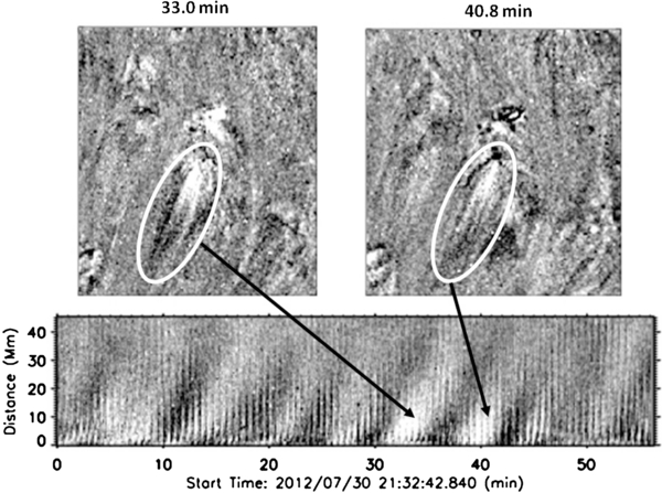
Figure 3. Running difference images (top) obtained during two of the brightest tracks in the space/time map (bottom), revealing the spikelike character of the ejections that produced those tracks. The images and space/time map are displayed at approximately the same spatial scale.
Download figure:
Standard image High-resolution imageNext, we extend the path outward from a center of activity and see what happens as successive plumes are encountered. The lower panel of Figure 4 shows a jmap, obtained with a similar 3.0 Mm slit and a path that encounters two plumes in the leading part of an old northern hemisphere active region on 2013 March 29. The path is indicated by the (yellow) dashed line running from lower left to upper right in the upper panel. In this jmap, the tracks occur in two partitions—one (0–75 Mm along the path) corresponding to the first plume and the other (75–150 Mm along the path) corresponding to the second plume. The boundary at 75 Mm is indicated by a small circle (red in the on line version) along the dashed path in the Fe xii image. In the first partition, the speeds are ∼90 km s−1, sometimes decreasing to about 40 km s−1. In the second partition, the speeds tend to be faster and show no obvious deceleration from values ∼110 km s−1. Also, there is no apparent phase relation between these two sets of tracks. Thus, it appears that each plume is the source of its own independent motions and that these separate motions create the impression of a continuous flow along the direction of the large-scale field.
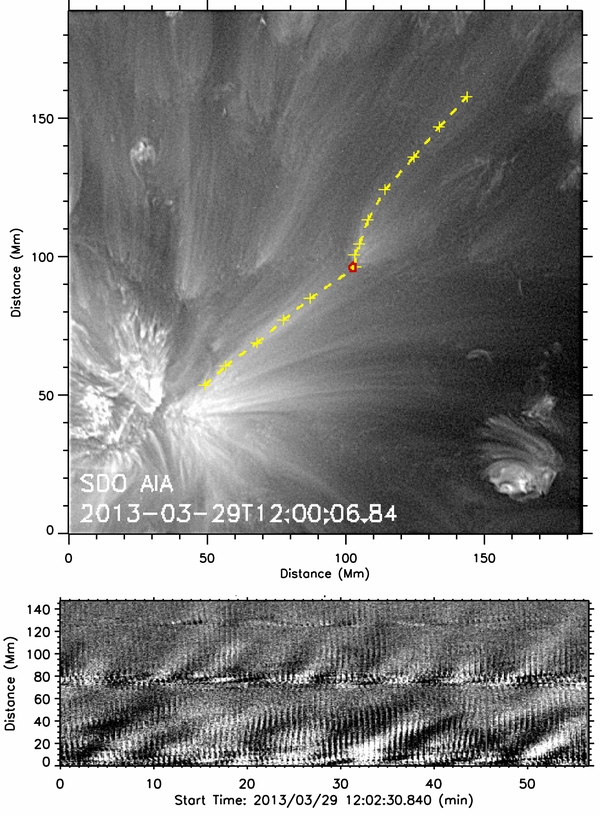
Figure 4. Fe xii 193 Å image (top) and a jmap (bottom) obtained for the dashed path through the region of plumes. In the 193 Å image, the red dot indicates the nose of the second plume where the discontinuity occurs at about 75 Mm along the track. The jmap slit had the same 3.0 Mm width used in the previous figures.
Download figure:
Standard image High-resolution imageFigure 5 provides another example, comparing 171 Å and 193 Å observations of plumes in a coronal hole on 2013 February 11. An HMI magnetogram (not shown here) indicates that these plumes extend from unipolar flux concentrations in a trailing region of positive polarity in the northern hemisphere. The top panels show the dashed path winding through the plumes in an Fe xii 193 Å image (left) and an Fe ix 171 Å image (right). As before, the separation of the individual tracks indicates the 3.0 Mm width of the slit used for the jmap. Although the plumes are shown much more clearly in the 171 Å image than the 193 Å image, the tracks of the repeating motions are only visible in the 193 Å jmap (middle panel), which contains three partitions of positively slanted tracks, occurring at distances of about 75 Mm (indicated by a small red circle in the upper panels) and 100 Mm along the track. The boundary at 100 Mm corresponds to a very faint plume and is not marked on these images. The slopes of the tracks seem to increase systematically from about 115 km s−1 for the first partition to 130 km s−1 for the third partition. In general, the tracks are not in phase, which further suggests that the coaligned plumes are contributing independent motions along the direction of the large-scale field. (In a few cases, tracks in the second partition extend into the very weak third partition, whose plume is so weak that it is hardly visible at 100 Mm along the track. This is what one would expect in the limit of a vanishingly weak field.)
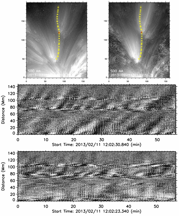
Figure 5. Fe xii 193 Å (left) and Fe ix 171 Å (right) images, and their respective jmaps (middle and bottom) for an identical (dashed) path along coronal hole plumes. The 193 Å jmap shows three cells of slanted tracks, which are not reproduced in the 171 Å jmap, despite the greater visibility of the 171 Å plumes.
Download figure:
Standard image High-resolution imageBy comparison, the 171 Å jmap (bottom panel) is dominated by poorly defined features. Our running difference image movies support this result. The 193 Å movie shows the repeated ejection of diffuse clouds from the base of each plume along this path, giving a clear impression of propagating motion, but the 171 Å movie does not. On the other hand, for a path through the brightest part of the first plume, the 171 Å movie shows a succession of bright ejections. Thus, the 171 Å and 193 Å brightness variations are not the same everywhere on the Sun, and the properties of the associated jmaps depend critically on the location of the path used for tracking. In Figure 5, the path through the collection of plumes was simply better suited for detecting 193 Å motions
Outside coronal holes, the cellular plumes are more visible in 193 Å images than in 171 Å images (Sheeley & Warren 2012), and the jmaps reflect this difference. The top panels of Figure 6 contain identical views of the northern edge of a coronal hole on 2013 August 14 with the jmap track superimposed. These dashed lines are double, not because they refer to the slit width (which was 4.7 Mm), but because the track reversed suddenly and moved back outward nearly along the inward path. In this way, the relatively wide paths overlap substantially and give a nearly symmetric chevron-like set of tracks, as shown by the 193 Å jmap in the middle panel. By comparison, the 171 Å images produced a jmap (bottom panel) dominated by the noisy changes of cooler features in the lower atmosphere.
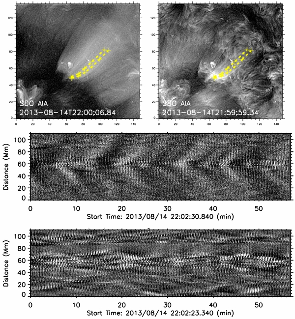
Figure 6. Identical views of the north edge of a 2013 August 14 coronal hole, as seen in Fe xii 193 Å (upper left) and Fe ix 171 Å (upper right). The dashed lines are separate segments of the folded path used to make the jmaps. The slit width was 4.7 Mm, which caused the segments of the path to overlap. The Fe xii jmap (middle) has faint tracks that repeat at intervals of five to seven minutes with slopes of ∼100 km s−1, whereas the Fe ix jmap (bottom) has disorganized tracks whose slopes are less than ∼25 km s−1.
Download figure:
Standard image High-resolution imageAlthough the jmap in Figure 6 was obtained using a 4.7 Mm slit width, the same result was obtained previously with a 3.0 Mm slit. In general, we have found that the jmap characteristics are relatively insensitive to such variations of slit width. For nominal widths, the main effect is a variation of contrast associated with the filling factor of the slit. Our observation that narrow slits give higher contrasts than wide slits seems to confirm that we are tracking narrow features.
3.2. Tracking Waves in Sunspots
Next, we turn our attention to sunspot waves as a second example of how our tracking procedure can be applied. Because the amplitudes of the waves are small (about 5% of the background intensity), we continued to average three consecutive frames. However, we reduced the lag of these averaged frames from four to two. This gave an effective lag of 72 s to our running difference images and provided an approximate match to the 78 s half period of these 2.6 minute waves. As discussed in Appendix A, this match ought to maximize the visibility of the waves in the running difference images and their jmaps. Although we could have obtained higher spatial resolution with a three-frame lag of two-frame averages, we found empirically that the two-frame lag of three-frame averages provided a better compromise between spatial resolution and sensitivity.
As mentioned earlier, recent improvements to the JSOC software have made it possible for us to examine many different sunspots in various stages of growth and disk position and in a variety of different spectral bandpasses. In this study we will only include observations of a single large (54 Mm diameter) sunspot during part of its transit across the Sun during 2013 November 14–18, and will leave the remaining observations of this and the other sunspots to a later more focused paper. However, we would like to mention that by experimenting with all of the AIA spectral bandpasses, we found that the main properties of the resulting jmaps fell into three basic types: jmaps whose tracks showed large accelerations (171 Å), jmaps of coronal motions with less acceleration or with deceleration (193 Å, 211 Å, and 131 Å), and jmaps of chromospheric tracks (304 Å and 1600 Å). Consequently, in this paper, we will mainly use the 171 Å, 193 Å, and 304 Å bands to describe the properties of the waves in sunspots.
Figure 7 compares HMI continuum observations of this sunspot together with corresponding AIA 171 Å images and lagged difference images. The 171 Å images show bright coronal features, rooted in the sunspot, and changing their aspect as solar rotation carries the spot from 50° east of central meridian on November 14 to the central meridian on November 18. By November 18, the coronal intensity distribution over the sunspot was split almost in two with bright emission on the northwest side and hardly any emission on the southeast side. Consequently, on this day, the strong difference signal was concentrated in the northwest sector of the sunspot, and only a weak (but important) signal occurred in the southeast. The right panel (middle row) shows three concentric waves extending upward along the plume coronal structure. A close examination of this figure reveals that these wave fronts become farther apart as they progress outward, which means that the waves are accelerating. Later in this section, we will use jmaps to show this acceleration more clearly and to measure its value. For the moment, we simply note that the average separation of these wave fronts is about 9 Mm (based on the 54 Mm diameter of the sunspot). For waves with a period of 2.6 minutes, this corresponds to an average speed of 58 km s−1.
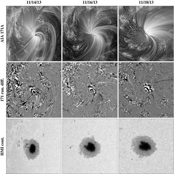
Figure 7. Sequence of AIA 171 Å coronal images, running difference images (with 72 s lags), and HMI continuum images, showing the wave patterns from a 54 Mm sunspot as solar rotation carried it from 50° east of central meridian on 2013 November 14 to the central meridian on 2013 November 18. In each running difference image, two to three concentric wavefronts are visible expanding outward along the 171 Å coronal fan, corresponding to an average wavelength ∼9 Mm. During November 14–18, these wave patterns rotated clockwise from ∼30° east north to ∼30° west of north due to the changing perspective of the coronal fan.
Download figure:
Standard image High-resolution imageMeanwhile, we call attention to some additional characteristics of this evolution. First, we note the changing aspect of the coronal intensity distribution, which began on the east side of the spot and ended up on the west side. The coronal wave patterns made a similar change, rotating clockwise from ∼30° east of north to ∼30° west of north during November 14–18. For such a long-lived leader sunspot, we would not expect the topology of the magnetic field to change significantly in such a short time. Thus, we suppose that these changes were due to the changing orientation of the structures as solar rotation carried them across the solar disk. Second, we consider the other half of the sunspot region where the coronal plumes are not visible. We shall see later that running penumbral waves (Zirin & Stein 1972) are present here. With some effort, one can see some of the wave fronts even in these 171 Å images, and especially in the He ii 304 Å running difference image in the next figure.
Next, in Figure 8, we focus on the observations of November 18. The top row of this figure shows the sunspot in the HMI continuum (left), and in the AIA bands of 171 Å (middle), and 193 Å (right). The middle row shows running difference images in He ii 304 Å (left), Fe ix 171 Å (middle), and Fe xii 193 Å (right), all free of the obscuring dashed lines that indicate the jmap path in the bottom row. Now, with some effort, one can see the chromospheric wave fronts in the non-plume part of the sunspot, especially in the He ii 304 Å image. Also, note that the coronal waves are smaller and less extended in the 193 Å image than in the 171 Å image. The jmap path extends from upper right to lower left, reaching the plume side of the sunspot first and then the non-plume side. In the sunspot image, the separation of the dashed lines indicates the 3.0 Mm width of the slit, which is small compared to the 54 Mm diameter of the sunspot.

Figure 8. Nearly simultaneous images of the same 54 Mm sunspot and its coronal plumes at 17:14:35 UT on 2013 November 18 as seen in the HMI continuum (upper left), and in the AIA passbands of 171 Å (upper middle) and 193 Å (upper right). In the second row, difference images, obtained in 304 Å (left), 171 Å (center), and 193 Å (right), show the bright coronal waves and the faint chromospheric waves, unobscured by the dashed yellow lines (bottom row) that mark the path used for our jmaps. In the sunspot image, the extra double lines indicate the 3.0 Mm width of the jmap slit.
Download figure:
Standard image High-resolution imageFigure 9 compares the jmaps obtained in He ii 304 Å (top) and in Fe ix 171 Å (bottom), cropped to the outer edge of the penumbra as shown in the abbreviated jmaps of the HMI continuum intensity at the right of each jmap. Several aspects of this figure are clear: First, on the non-plume side of the sunspot (above 24 Mm), the 171 Å tracks have lower contrast than the 304 Å tracks, but are otherwise the same. These two sets of tracks begin in the umbra and decelerate through the penumbra until they become part of a "criss-cross" of tracks that move with slow speeds in both directions. (This leads us to wonder whether these crossed tracks indicate damped reflections from the outer boundary of the penumbra, but we will leave that question to future work). As we shall see later in this paper, these slow speeds are ∼7–8 km s−1, which is comparable to the sound speed in the lower atmosphere. Because the He ii tracks refer the chromosphere, it is likely that the identical 171 Å tracks also refer to the lower atmosphere (either the chromosphere or the nearby transition region). This raises the question of whether the emission comes from relatively hot, 0.8 MK Fe ix 171 Å ions located at chromospheric heights, or whether the emission originates from a lower-temperature spectrum line in the 171 Å bandpass.
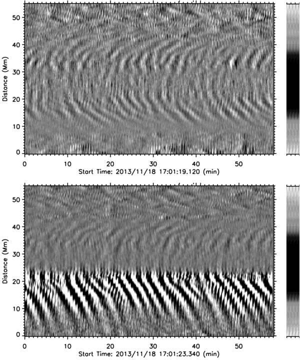
Figure 9. He ii 304 Å (top) and Fe ix 171 Å (bottom) jmaps for the path in the previous figure, cropped at the outer edge of the penumbra as shown to the right. On the "plume-free" side of the sunspot (>24 Mm), the 304 Å and 171 Å tracks are virtually identical, which means that they have a common origin in the chromosphere. On the "plumeward" side (<24 Mm), the 171 Å tracks accelerate outward into the corona and the 304 Å tracks decelerate.
Download figure:
Standard image High-resolution imageSecond, on the plume side of the sunspot (below 24 Mm), the 171 Å tracks are strong and they accelerate, whereas the weaker 304 Å tracks decelerate. As described below, the speeds of the 171 Å motions accelerate from about 40 km s−1 to values in the range 60–100 km s−1. At each time, one can see a maximum of three bright tracks over a distance of about 20 Mm, corresponding to an average separation of about 9 Mm, consistent with our earlier impression from the appearance of the waves in Figures 7 and 8. These accelerating tracks begin at the same space/time coordinates as the decelerating He ii 304 Å chromospheric tracks, which means that the two sets of tracks are different responses to the same umbral disturbance. Thus, we are observing two different waves from the same source—one that decelerates as it moves through the chromosphere and another that accelerates as it moves upward into the corona.
Next, in Figure 10, we compare the He ii 304 Å jmap (top) with a C iv/1600 Å jmap, again cropped to the outer edge of the penumbra. These two jmaps show remarkably similar sets of decelerating tracks on both sides of the sunspot (i.e., above and below the coronal boundary at 24 Mm). These similar sets of decelerating tracks are consistent with the decelerating tracks observed previously in chromospheric lines (Georgakilas et al. 2000; Rouppe van der Voort et al. 2003), and what we might expect for lines that are formed in the chromosphere and transition region. This deceleration causes the tracks to become closer together as they move outward through the penumbra. In the 1600 Å jmap, the track separation decreases from 5 Mm at the start to 1–2 Mm midway through the penumbra. This crowding of wave fronts is sometimes visible directly in our running difference image movies.
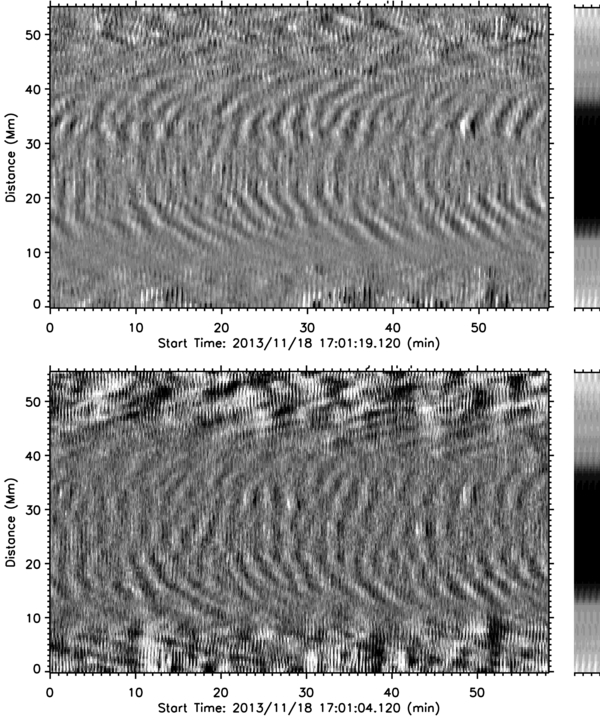
Figure 10. He ii 304 Å (top) and C iv/1600 Å continuum (bottom) jmaps, cropped at the outer edge of the penumbra, showing virtually identical decelerations characteristic of the chromosphere. As before, the continuum intensity profile (right) shows the location of the umbra and penumbra along the cropped path.
Download figure:
Standard image High-resolution imageIn Figure 11, we compare jmaps in the two coronal emissions at 171 Å (top) and 193 Å (bottom). Virtually identical decelerating tracks are visible on the non-plume side of the sunspot, so that the 171 Å and 193 Å radiation must originate in the lower atmosphere (chromosphere and transition region). On the plume-side of the sunspot, both sets of tracks are strong, but the 171 Å tracks are longer, extending ∼20 Mm to the outer edge of the penumbra, whereas the 193 Å tracks fade out after about 15 Mm. Also, the 171 Å tracks show more acceleration than the 193 Å tracks, some of which decelerate as they extend outward into the penumbra. This difference is significant because the bright decelerating tracks cannot be attributed to hypothetical contributions from faint low-temperature lines in the 193 Å bandpass. These decelerating 193 Å tracks must originate in high-temperature (i.e., ∼1.2 MK) Fe xii plasma that lies close to the chromosphere.

Figure 11. 171 Å (top) and 193 Å (bottom) jmaps for the path used in the previous figure, showing that the bright coronal tracks (<24 Mm) are not the same in the 171 Å and 193 Å images. Although the two sets of tracks emerge from the same locations, the 193 Å tracks are shorter and often decelerate, while the 171 Å tracks accelerate.
Download figure:
Standard image High-resolution imageBecause the unsubtracted 171 Å and 193 Å images in Figure 8 look quite similar, it is surprising to find bright tracks that accelerate in 171 Å, but decelerate from the same location in 193 Å. We can understand such differences in the 304 Å and 171 Å jmaps because they refer to completely different parts of the solar atmosphere—the chromosphere and the corona, respectively. This 171 Å–193 Å comparison is telling us that along this tracking path, the 171 Å radiation is coming from a much greater height in the atmosphere than the 193 Å radiation. This is what we would expect if the 171 Å radiation originates in an outward extending coronal fan while the 193 Å radiation comes from a low-lying coronal loop. In the future, we plan to construct differences between the 171 Å images and the 193 Å images to see if we can detect the individual features that produce these two different kinds of tracks.
Figure 12 contains measurements of tracks obtained from the 171 Å and 304 Å jmaps in Figure 9. We fit the 304 Å deceleration measurements with a speed profile which decreased exponentially toward a final asymptotic value. In this case, the initial speed was 42 km s−1, and final speed was 8.4 km s−1, or roughly the sound speed close to the Sun. The decay time was 167 s, corresponding to an initial acceleration of 202 m s−2. We seldom obtained a successful fit to the measurements of accelerating motions using an exponentially decreasing velocity profile. Consequently, we used a quadratic height/time profile for the 171 Å accelerating motions. In this case, the speed increased linearly with time from 30 km s−1 at the start to 60 km s−1 after 500 s, corresponding to a constant acceleration of 63 m s−2. As we shall see, the measurements of accelerating motions varied more from event to event than the measurements of the decelerating motions. The larger variations may indicate a greater sensitivity to geometric projection effects as well as measurement limitations caused by the relatively shorter times that the accelerating tracks could be observed before they faded out.

Figure 12. Measurements of tracks in the 171 Å and 304 Å jmaps on 2013 November 18, comparing the speeds and accelerations of the coronal and chromospheric waves. (top): 171 Å track, fit with a quadratically increasing distance. (bottom): 304 Å track, fit with an exponentially decreasing speed.
Download figure:
Standard image High-resolution imageNext, we consider observations on 2013 November 15, when the coronal plumes seemed to be spread uniformly around the sunspot, as shown in Figure 13. In this case, we chose a path that moved inward along the coronal fan at the north edge of the sunspot. On leaving the sunspot, we let the path curve westward and southward along the short loops that might lie close to the surface. (Because we cropped the path at the outer edge of the penumbra, the resulting short segment was essentially straight, so a curved slit was really not necessary in this case.) Thus, the path begins with the coronal fan and ends with the short loops, both of which gave bright tracks in the jmaps.

Figure 13. Sunspot and its coronal plumes at 16:33:11 UT on 2013 November 15 when the plumes are visible more uniformly around the spot. Top row: HMI continuum (left), 171 Å (middle) and 193 Å (right), showing the sunspot and its coronal plumes. Middle row: difference images in 304 Å (left), 171 Å (center), and 193 Å (right), showing the faint chromospheric and bright coronal waves. Bottom row: the same images with dashed lines marking the jmap path. In the sunspot image, the extra lines indicate the jmap slit width.
Download figure:
Standard image High-resolution imageFigure 14 compares jmaps in 171 Å (top) and 193 Å (bottom). It is significant that these tracks are strong on both segments of the jmap path (i.e., for the plumes below 20 Mm and the short loops above 20 Mm). This means that we cannot attribute the decelerating tracks in the short loops to a weak, low-temperature line in the 193 Å bandpass. The obvious 193 Å deceleration must originate in 1.2 MK Fe xii emission from the low-lying coronal loops. In contrast, the coronal fan (below ∼20 Mm) shows accelerating tracks in both jmaps, but extending farther outward in 171 Å than in 193 Å.
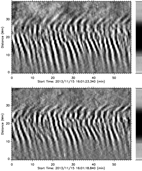
Figure 14. 171 Å (top) and 193 Å (bottom) jmaps for the path shown in the previous figure, cropped at the outer edge of the penumbra (as indicated on the right) and with relabeled distance scales. The interval 0–20 Mm marks the base of the fan where the tracks accelerate, and the interval 20–40 Mm indicates the legs of the short loops where the tracks decelerate.
Download figure:
Standard image High-resolution imageFigure 15 shows that the decelerating motions in the low-lying 193 Å loops (i.e., above 20 Mm) are similar to those seen in the chromospheric emission from 304 Å. However, on the fan side of the sunspot (below 20 Mm), the bright 193 Å tracks show the acceleration characteristic of motions outward from the Sun, while the 304 Å chromospheric tracks decelerate as they fade.
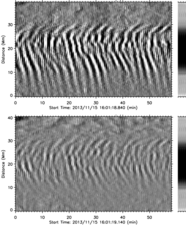
Figure 15. 193 Å (top) and 304 Å (bottom) jmaps, for the path described in the previous figures. The He ii 304 Å tracks decelerate in both segments of the path, as expected for motions close to the surface, but the Fe xii 193 Å tracks accelerate outward in the fan (0–20 Mm) and decelerate in the short, low-lying loops (20–40 Mm).
Download figure:
Standard image High-resolution imageIn Figure 16, we show measurements of these accelerations and decelerations on November 15. The quadratic fit to an accelerating track along the coronal plume gave an initial speed of 38 km s−1 increasing linearly to a final speed of 100 km s−1 after 280 s, corresponding to a constant acceleration of 215 m s−2. This final speed is somewhat greater than the final speed of 60 km s−1 that we obtained for the plume motions on November 18, and illustrates the range of values that we typically obtain for the accelerating motions (i.e., speeds increasing from ∼40 km s−1 to values in the range 60–100 km s−1 before the track fades out).

Figure 16. Measurements of tracks in the 171 Å jmap on 2013 November 15, comparing speeds and accelerations of the coronal and chromospheric waves. Top: accelerating track, fit with a quadratically increasing distance. Bottom: decelerating track, fit with an exponentially decreasing speed.
Download figure:
Standard image High-resolution imageIn contrast, the lower panels of Figure 16 show measurements of a decelerating track on November 15, in which the speed decreased exponentially from an initial value of 49 km s−1 toward an asymptotic value of 7.4 km s−1 on an e-folding time of 167 s. This corresponds to an initial deceleration of 252 m s−2. These values are very close to the ones obtained in Figure 12 for a decelerating track and illustrate the relatively low scatter that we have found for the decelerations. Thus, in the lower atmosphere, the speeds decrease from initial values ∼40 km s−1 toward final asymptotic values of 7–8 km s−1 on e-folding timescales of about 2.5 minutes.
It is interesting that the e-folding time is ∼2.5 minutes. This time is essentially the same as the 2.6 minute repetition period of the waves, which means that each wave reduces its deceleration to 1/ (37%) of its initial value by the time that the next wave starts out from the umbra. The deceleration falls to 13.5% and 5.0% of its initial value by the start of the third and fourth wave, respectively. Thus, at a given moment, all of the waves except the last three would have reached their asymptotic speeds of 7–8 km s−1, and their wavefronts would be separated by only 1.2 Mm (i.e., the distance they move during a repetition time).
4. SUMMARY AND DISCUSSION
We have developed a new procedure for tracking proper motions of faint XUV coronal intensity across the solar disk, and we have used this procedure to investigate the apparent large-scale motions across unipolar magnetic regions and the smaller-scale wavelike motions in sunspots. Here, we discuss these results separately.
4.1. Cellular Plumes
We found that the apparent motion across unipolar regions is not a continuous flow, but instead is a sequence of independent quasi-periodic motions caused by the repeated ejection of bright features from the magnetic flux concentrations at the bases of cellular plumes. The brightness enhancements repeat on timescales of about six minutes and move along the field of the individual plumes with speeds of about 100 km s−1 and corresponding separations ∼36 Mm. The result is an apparent flow down the gradient of the large-scale field, similar to the "flow field" that one might infer from the directions of the individual cellular plumes (Sheeley et al. 2013; Wang et al. 2013b) or from Hα observations of chromospheric fibrils (Foukal 1971; Sheeley 1981).
Sometimes the tracked features are linear spikes, perhaps like Type II spicules (de Pontieu et al. 2007; De Pontieu & McIntosh 2010; De Pontieu et al. 2011, 2012), but these spikes along the jmap path may be part of a wider release that ultimately becomes directed along the background magnetic field. In the future, we hope to test this idea by comparing simultaneous jmaps obtained for paths that are systematically placed at position angles around the base of the plume. Meanwhile, we note that the phases of the tracks seems to be uncorrelated from one cell to the next. (In the 193 Å jmap of Figure 5, we noticed that some of the tracks of one cell extended through a second, very faint cell. This is what we would expect if the field of the second cell were very weak.) This lack of correlation implies that the motion is more like a system of independent cellular releases than a continuous flow along the field.
The apparent large-scale motion is clearly visible in time-lapse movies made with suitably lagged 193 Å images, but the motion is not visible with 171 Å images. The reason for this discrepancy is that the coronal cells have their greatest visibility at the 1.2 MK temperature of the Fe xii 193 Å emission line. The cells are not visible at the 0.8 MK temperature of Fe ix 171 Å, as shown in Figure 6 and in a previous paper by Sheeley & Warren (2012). In this paper, we captured the motion in jmaps of individual cells as well as in a series of cells. It is reassuring that the speeds and periods that we obtained for the cellular plumes in unipolar magnetic regions are consistent with the values that have been obtained previously in bright active region fans (De Moortel 2005; Tian et al. 2011b; De Moortel & Nakariakov 2012; Wang et al. 2013a) and in plumes in coronal holes (Deforest & Gurman 1998; McIntosh et al. 2010; Krishna Prasad et al. 2011). This makes us wonder whether a single mechanism might apply to all of these coronal structures, rather than the separate interpretations in terms of ejections (for the fans) and waves (for the plumes) that sometimes appear in the literature (e.g., Doschek et al. 2008; Deforest & Gurman 1998).
The observations described here support the idea that each flux concentration in a unipolar magnetic region is the source of repeated intensity bursts whose ejecta may initially move in all directions, but eventually be guided along the magnetic field of the plume (Sheeley & Warren 2012). As discussed in Appendix B and illustrated in Figure 17 for an idealized model, the initially "radial" field lines of the monopole are bent "downfield" to become part of the uniform background field. Thus, ejections in the downfield direction will continue in that direction and form the central part of the tail, but ejections in the upfield direction will be turned around and sent along the outer layer of the tail. The uniform field of the tail then becomes the background field for the next plume, and the process repeats to form a highway of apparent flow around the Sun. The cellular plumes and their associated flux concentrations are the building blocks of this highway of apparent motion.

Figure 17. Field lines for a concentration of positive-polarity flux in a uniform background field that points left to right along the x axis. Lengths are expressed in units of the standoff distance between the null point and the flux concentration at the origin of the coordinate system. Field lines through the null point separate the monopolar flux from the background flux that sweeps around it to form a uniform downstream field. The monopolar flux, Φ, standoff distance, s, and background field strength, B0, are related by π(2s)2B0 = Φ.
Download figure:
Standard image High-resolution imagePreviously, we suggested that cellular plumes may be similar to the classic plumes in coronal holes (Sheeley & Warren 2012). This returns us to the question of whether the proper motions of these two kinds of plumes have a common origin. Wang et al. (1997) and Raouafi & Stenborg (2014) have suggested that plumes may be produced during the reconnection between field lines from the unipolar flux concentration and a wandering element of opposite polarity. Although such episodic reconnections may create the occasional jets that occur during the formation of a plume, it seems doubtful that they could be responsible for sustained five to eight minute quasi-periodic motions within the plume.
The similar repetition times of photospheric and coronal motions are a compelling reason to look for a link between these oscillations. Jefferies et al. (2006) have suggested that the network fields provide magnetoacoustic portals for photospheric waves, and Cally & Moradi (2013) have considered a mechanism for converting fast-mode waves to slow-mode waves in regions where the fields are sufficiently inclined to the surface. However, according to this idea, slow-mode waves with periods in the range 5–10 minutes would not propagate upward unless the tilt angle were ∼60°–70° from the vertical, which seems much greater than what we infer from cellular plumes. Also, the spicular character of the ejections makes us wonder whether a vertical field might provide a quasi-rigid boundary for waves to splash upward like water at the posts of a pier.
4.2. Sunspot Waves
We made running difference movies and jmaps of a large, stable, leading-polarity sunspot at a variety of wavelengths and disk positions. These observations showed bright waves, accelerating outward along a coronal structure that was rooted in that sunspot, and fainter chromospheric waves, decelerating as they moved outward through the penumbra. The coronal and chromospheric tracks began from the same points in the space/time map, which means that they were produced by the same disturbance at that location. We found that the speed of the chromospheric waves decreased exponentially from ∼40 km s−1 to 7–8 km s−1 in about 2.5 minutes, corresponding to an initial deceleration of 220 m s−2. The speed of the coronal waves also began around 40 km s−1, which is consistent with the idea that the two waves have common origins.
In our jmaps of chromospheric waves, the decelerations were shown by the rapid bending and flattening of the tracks. This caused the tracks to become crowded more closely together along the slit, corresponding to a decrease in wavelength. For a constant period of 2.6 minutes, a nominal deceleration from 40 km s−1 to 7.5 km s−1 would correspond to a wavelength change from 6.2 Mm to 1.2 Mm. In some of our jmaps, like the C iv/1600 Å jmap in Figure 10, we could measure 1.8 Mm separations for tracks that were about 7 Mm from the outer edge of the penumbra. However, in this outer part of the penumbra, the jmaps became noisy due to the competing contributions of inward moving tracks with speeds that were also ∼7–8 km s−1. Because the speed of the outward tracks did not seem to be approaching zero at the outer boundary of the penumbra, we wondered whether these inward tracks of comparable speed might be reflections of the outgoing waves. However, we will leave this question to a future, more focused study.
The measured accelerations of the coronal waves showed more scatter than the decelerations. This resulted in a broad distribution of final speeds, ranging from 60 km s−1 to 100 km s−1 or even more. We suppose that this variation depends on the fading length of the height/time track as well as variations in the inclination of the plume above the sky plane. (Recall that these measurements refer to the sky-plane component of motion, and have not been corrected for the plume's inclination.) For observations near disk center (like those in Figures 9 and 14), the 171 Å tracks of accelerating motions were visible for about 20 Mm and therefore did not extend much beyond the outer edge of the penumbra of this 54 Mm sunspot. However, for observations of other sunspots at the extreme limb (not shown here), the 171 Å accelerating tracks were clearly visible for about 10–15 Mm above the limb. In any case, the observed accelerations imply that the wave fronts ought to separate with height, as we observed in running difference images like those in Figures 7, 8, and 13. For a nominal acceleration from 40 km s−1 to 80 km s−1, the wavelength ought to increase from 6.2 Mm to 12.4 Mm, consistent with the ∼9 Mm value that we estimated from the images in these figures and with the 14 Mm spacing of some tracks in the 171 Å jmap of Figure 14.
Because the chromospheric and coronal waves emerged from the same locations in our space/time maps, the repetition periods of these two kinds of waves had a common value. By counting the number of waves in the 57 minute length of the jmap, we obtained a period of approximately 2.6 minutes. In Appendix C, our Fourier transform of the 171 Å jmap on November 18 gave 2.6 minutes at the coronal base, but with a slight increase of period (decrease of frequency) with height or radial position in the sunspot. The decrease was from 0.42 minute−1 to 0.32 minute−1, corresponding to an increase in period from 2.4 minute to 3.2 minute. Expressed in mHz, the frequency decrease was from 7.0 mHz to 5.3 mHz, in rough agreement with He ii 304 Å measurements by Reznikova & Shibasaki (2012).
In our jmaps, a frequency decrease can only occur if there are fewer tracks to count as one progresses along the tracking path. One cause of this attrition is the preferential fading of some tracks with height (i.e., distance along the slit), so that only the brightest tracks remain to be counted. Sometimes even bright tracks leave the pack, either because they decelerate and are left behind, or perhaps because the motions change direction and leave the tracking path. This is another area in which we would expect to make progress by constructing a series of jmaps at closely spaced slit positions around the sunspot.
Another interesting result from the Reznikova & Shibasaki (2012) paper is their discovery that for one sunspot (on 2010 July 2) enhanced three minute oscillations are not visible over the umbra, but are visible in the fan structure on the west side of that umbra. Our 171 Å observations of the leader sunspot on November 15 and 17 seem to show a similar effect—strong oscillations in the western fan, but only faint chromospheric oscillations in the non-fan part of the sunspot. Also, as indicated in Figure 7, this fan of waves appeared to rotate as solar rotation carried the sunspot across the Sun's disk. In the near future, we plan to apply our tracking procedure to the 2010 July 2 sunspot to see if we are observing the same effect as Reznikova & Shibasaki (2012), or whether the umbra of that sunspot lacked oscillations entirely.
G. Stenborg & T. Stekel (2012, private communication) have described AIA observations that associate the three minute waves in sunspot plumes with C iv/1600 Å brightenings at the roots of those plumes in the sunspot. Based on the virtual coincidence between the starting points of the tracks in C iv/1600 Å, He ii 304 Å, Fe ix 171 Å, and Fe xii 193 Å jmaps, it is clear that all of these waves have a common origin in the sunspot umbras. Time-lapse movies and space/time slices of chromospheric motions in the Ca ii 3934 Å and 8542 Å lines (Rouppe van der Voort et al. 2003; de la Cruz Rodríguez et al. 2013) indicate clearly that running penumbral waves originate with umbral flashes (Beckers & Tallant 1969), which therefore must be the common origin of the AIA chromospheric and coronal waves. Because umbral flashes are thought to occur when sub-photospheric waves reach the low-density umbral chromosphere and steepen into shocks (de la Cruz Rodríguez et al. 2013 and references contained therein), even the coronal parts of these sunspot waves must have a sub-photospheric origin.
5. CONCLUSION
We are left with a mental picture in which the flux elements of a unipolar magnetic region are like geysers, each producing repeated bursts at six to eight minute intervals, but uncorrelated in time with bursts from the other geysers in that region. The ejections often appear like giant spicules, initially moving outward in all directions from their sources, but then turning "downwind" in the direction of the large-scale magnetic field. The sky-plane speed is ∼100 km s−1, which is comparable to the sound speed in a 1 MK coronal plasma, and allows each fading ejection to reach (and be deflected by) the neighboring plume by the time that the next burst occurs. The lack of a phase correlation between the adjacent plumes prevents the formation of a correlated large-scale pattern, and the result is a collection of independent quasi-periodic motions. Despite this autonomy, the common direction of motion along the large-scale magnetic field links these independent motions together and gives the impression of a continuous chain of flow across the Sun.
In sunspots, the 2.6 minute disturbances are easily recognized as waves by their broad circular wavefronts moving outward from localized sources in the umbra. As the chromospheric component moves horizontally through the sunspot penumbra, it decelerates from an initial speed around 40 km s−1 toward an asymptotic value in the range 7–8 km s−1, which is the speed of sound in a 6000 K plasma. However, the coronal component accelerates as it moves upward, ultimately reaching speeds that are comparable to the 100 km s−1 speeds in cellular plumes. In sunspots, the tracks of the coronal and chromospheric waves start from the same space/time locations, which means that they must have a common origin in umbral flashes—the known source of the chromospheric waves.
We are grateful to Nathan Rich (NRL) for his continuing help in the development of software for observing and analyzing SOHO, STEREO, and SDO images. We are grateful to the AIA and HMI science teams for providing observations from the NASA SDO spacecraft, and especially to Sam Freeland (Lockheed), Todd Hoeksema (Stanford), Marc de Rosa (Lockheed), and Phil Scherrer (Stanford) for help with downloading the data. It is a pleasure to acknowledge Jack Harvey (NSO), Frank Hill (NSO), G. Stenborg (GMU), Yi-Ming Wang (NRL), and Peter Young (GMU) for useful scientific discussions. One of us (S.C.) acknowledges support from the Naval Research Enterprise Internship Program(NREIP) at NRL. Two of us (J.K. and M.N.) thank NRL for allowing us to participate in this research as NRL Student Volunteers. Financial support was provided by NASA and the Office of Naval Research.
APPENDIX A: INTERPRETING LAGGED DIFFERENCE IMAGES
Running difference images are used routinely to study motions in the outer corona. Their main effect is to remove the bright background intensity and enhance the subtle changes of intensity caused by outward (or inward) proper motions of material. The motions tend to be simple flows that are easily interpreted using the running difference images. In the Fe xii 193 Å corona, the motions are also faint (with intensity changes ≲5%), but in addition, they tend to be repetitive with periods ∼5–10 minutes. Thus, running differences may affect the visibility of these motions depending on the time lag that is used in their construction. Consequently, in this appendix, we provide a brief discussion of what one might expect running difference images to show when they are used to observe periodic disturbances in the XUV corona.
Let us begin with the simple case of a wave w(x, t) that remains positive like a pressure variation and depends on distance x and time t according to
where λ is the wavelength and τ is the period of the motion. In this case, the amplitude of the wave is always positive and varies from 0 to 1. How would this wave appear if it were observed with a running difference image using a time lag, Δt?
To see this, we define the lagged difference f(x, t) by

and evaluate it using the expression for w(x, t) given above. After some algebra, we find that
The lag, Δt, affects the amplitude and phase, but it leaves the wavelength and period (and therefore the wave speed) unchanged. As expected, the subtraction removes the ambient level so that the variation now changes sign during each period of motion. In the special case that Δt = τ/2, the phase πΔt/τ becomes π/2, the amplitude becomes 1, and f(x, t) reduces to
Thus, the original cosine-squared function w is converted to a cosine function f, which varies in phase with w, but changes from +1 to −1 instead of +1 to 0. By subtracting the images 180° out of phase, we enhanced the contrast by a factor of two and introduced dark (i.e., negative) areas in place of previously gray ones, but otherwise we left the images the same.
On the other hand, if we had used a lag equal to the full period of motion, τ, then the phase πΔt/τ would have been π, and the waves of that period would have vanished from the running difference function f. Of course, if the amplitudes of these waves were not constant, then a residual contribution would have remained after the subtraction. Nevertheless, the lag, Δt, determines which periods will stand out and which periods will be repressed in our movies and space-time plots. For the analysis of the motions in cellular plumes, we chose a lag of 144 s, which provides suitable resolution and contrast, and enhances waves with periods around five minutes. For sunspot waves, we used 72 s, which is close to the 1.3 minute half period of those waves.
Also, we would like to know what the running difference images would show if the input wave has components of different frequencies that are not harmonics of each other. Thus, as a second example, we consider an input wave composed of two cosine-squared waves of different frequencies ω1 and ω2, but equal amplitudes. We suppose that they travel at the same speed, v, determined by the local plasma conditions, so that their wavelengths λ1 and λ2 are related to their periods τ1 and τ2 by v = λ1/τ1 = λ2/τ2. In this case, we can express the wave w(x, t) as
Proceeding as before, we replace the cosine-squared terms with cosines of double angles and then add the cosines to obtain
where ω0 is the average of the two frequencies, (ω1 + ω2)/2, and Δω is their difference, (ω2 − ω1). This equation shows that when two different frequencies are present, the waves go in and out of phase, producing a high-frequency component that is modulated by a low-frequency envelope. Consequently, plots of constant w(x, t) will produce a series of space-time tracks whose strengths change gradually at the slow rate, Δω/2, of the low-frequency modulation, but whose slopes (and thus speeds v) remain unchanged.
Our next step is to see what the lagged difference does to this wave. Proceeding as before, we evaluate the difference w(x, t)–w(x, t − Δt) separately for the two components and then add them together to obtain
where ωjΔt/2 = (ω0Δt/2)[1 ± (1/2)(Δω/ω0)] with the minus sign to be used when j = 1 and the plus sign when j = 2. Thus, when there are two frequency components, the lagged difference changes the amplitude and phase of each component.
Earlier in this appendix, when we were analyzing a wave of one frequency, ω0, we chose a lag, Δt, equal to one-half the oscillation period at that frequency, so that ω0Δt = π. Now, that we have waves of two frequencies, ω1, and ω2, we chose a lag, Δt, equal to one-half of the oscillation period at the frequency, ω0, located mid-way between them. In this case, ω0Δt/2 = π/2, and the lagged difference function, f(x, t), becomes
Comparing this expression for f(x, t) with the corresponding expression for w(x, t), we see that the running difference removes the constant term and causes the magnitude to change sign by an amount that depends on the value of (π/4)(Δω/ω0), instead of varying from 1 to 0. If we suppose that the frequencies ω1 and ω2 correspond to periods of 10 minutes and 5 minutes, respectively, which span the range seen in our Fe xii jmaps, then the phase, (π/4)(Δω/ω0), is 30°. In this case, the lagged difference would have a relatively minor effect on the composite waveform, reducing its amplitude by 13} and shifting its phase by 50 s of time. Unlike the frequencies, which combine directly to give their average ω0, the periods combine inversely so that the lag, Δt, is given by the relation 1/Δt = 1/τ1 + 1/τ2, which is 3.33 minutes for individual periods of 10 minutes and 5 minutes. It is reassuring that for equal periods (and therefore a single wave), the value of Δt reduces to one-half their common value.
For completeness, we mention briefly the results of calculating the effect of the lagged difference on two waveforms composed of continuous frequency distributions. First, we considered what the lagged difference would do if the frequency spectrum were a Gaussian. The result was a damped wave, as we might have guessed by analogy with quantum states, which decay slowly for narrow energy levels and more rapidly for broader ones. Then we considered a continuous frequency spectrum that was centered around the frequency of the original cosine-squared distribution. Again, we obtained a decaying amplitude, but this time caused by a sinc function sin (Δωt/2)/(Δωt/2), rather than a Gaussian  . Clearly, continuous frequency distributions correspond to decaying waves.
Summarizing these examples, the important concept seems to be how long the waves last before they decay or are weakened by interference with other waves. Our calculations suggest that the lifetimes depend on the purity of the spectrum with the longest lifetimes occurring for waves that are composed of a single frequency and its harmonics. The calculations also suggest that for a suitable choice of lag, running difference images ought to show propagating disturbances with little distortion and to provide an accurate indication of their speeds.
APPENDIX B: MONOPOLE IN A UNIFORM BACKGROUND FIELD
As we have seen previously, coronal plumes extend upward from the network flux concentrations in a unipolar magnetic region, and lean in the direction of the horizontal component of the large-scale field (Sheeley & Warren 2012; Sheeley et al. 2013; Wang et al. 2013b). The fine-scale threads of each plume seem to be swept "downstream", as if they were tracing the field lines of a monopole placed in an external horizontal magnetic field. To illustrate this configuration, we will now calculate the field of a localized source of flux Φ placed in a uniform magnetic field of strength B0. We assume that the monopole has a positive polarity and is located at the origin of an xy coordinate system whose x-axis defines the direction of the background field. (The same result would be obtained for a negative-polarity flux concentration, provided the direction of the x-axis is reversed.) Together, the background field and the monopole combine to give the composite field B(x, y),

where ex and er are unit vectors in the x-direction and r-direction, respectively, and r is the radial distance from the flux concentration to the field point (x, y). The fields of these two components oppose each other to the left of the monopole where x is negative and reinforce each other to the right where x is positive. By setting B(s, 0) = 0, we see that the null point's "standoff" distance, s, from the origin is given by

If we express all distances in units of s and all field strengths in units of B0, then Equation (9) takes the dimensionless form

This equation gives a uniform field in the x-direction at large distances upstream and downstream from the monopole, and an outward-directed inverse-square field surrounding the monopole.
To obtain the field lines for this configuration, it is convenient to use polar coordinates (r, θ) and to evaluate the field components, Br and Bθ, as follows:


In this case, the field-line equation becomes
This equation can be rewritten as

and easily integrated to obtain
where k is a constant of integration. Introducing a field-line parameter λ, defined by λ2 = 2(k+1), and recognizing that y = rsin θ and x = rcos θ, we obtain parametric equations for x and y in terms of the angle θ and the parameter λ,

and

From the first of these two equations, we see that y2 has its maximum value when θ = 0, and that this maximum value is λ2. Thus, each field line is defined by its asymptotic height, λ, above (or below) the x axis as x → ∞.
Figure 17 shows a sample of field lines plotted in uniform θ steps of 45° and in uniform y steps of 0.5 when θ = π. We can see that the field lines of the monopole are "swept back" into a "cylindrical" region that is separated from the background field lines by a separatrix that passes through the null point at the nose of this configuration. In the xy plane, this separatrix corresponds to a pair of field lines with λ = ±2, as one can see by setting y = 0 and θ = π in the equation for y2. This means that 2s is the radius of the cylinder which asymptotically contains all of the monopole's flux Φ = π(2s)2B0. Equivalently, the standoff distance, s, at the upstream nose of this structure is one-fourth the width of the downstream "tail". Similarly, because  = Φ/2, the field lines with λ =
  separate the monopolar flux into two equal parts with their field lines initially pointing "upstream" and "downstream" from the monopole.
These results provide a way of deducing the horizontal field strength in the corona from a knowledge of the amount of flux in the monopole together with spatial measurements of the associated plume. In particular, if a typical network flux of 0.2 × 10²¹ Mx were swept into a cylinder of 30 Mm diameter (or compressed to a standoff distance of 7.5 Mm), we would infer a horizontal field strength of about 32 G.
APPENDIX C: FOURIER TRANSFORMS OF JMAPS
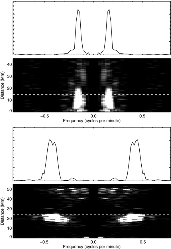
Figure 18 shows Fourier transforms of the 193 Å jmap of a cellular plume in Figure 2 (upper panels) and the 171 Å jmap of sunspot waves in Figure 9 (lower panels). Because there are few cycles in the spatial dimension, we did not transform the jmaps in that dimension. Instead, we transformed the jmaps in the time dimension only, and expressed the resulting spectral power as a function of temporal frequency (in cycles per minute) and distance along the slit (in Mm). In the 193 Å map, the power is concentrated around 0.16 minute−1 (6.3 minutes) without much change with distance along the slit. The frequency decreases slightly toward the top of the slit where the power is less. This spectral migration occurs because the tracks fade with distance along the slit so that only the longest and brightest remain to be counted. The associated line plot shows the power along the dashed line. Its peak occurs at 0.16 minute−1, corresponding to a period of 6.3 minutes.
Figure 18. Spectral power in the 193 Å jmap of Figure 2 (top) and in the 171 Å jmap of Figure 9 (bottom) as a function of temporal frequency and slit position, showing that the motions in cellular plumes and the waves in sunspots have periods ∼6.3 minutes and ∼2.6 minutes, respectively. In each case, a line plot shows the power along the dashed line.
Download figure:
Standard image High-resolution image
The 171 Å map has been scaled to show the bright coronal waves below 24 Mm. Here, the power begins at 0.42 minute−1 (2.4 minutes) and drifts to 0.32 minute−1 (3.2 minutes) at a location 15–20 Mm farther outward along the slit. From an examination of the jmap in Figure 9, we see that this drift in frequency results from the attrition of tracks with height, so that fewer of them remain to be counted at the greatest heights. For this jmap, some tracks leave the pack due to their preferential fading with distance along the slit, while others may leave as their motion takes them off the tracking path. This is a subject for future study.
The associated line plot shows the power along the dashed line, close to the base of the coronal fan. Although the distribution is centered around a frequency of 0.42 minute−1 (2.4 minutes), it is relatively broad with a range 0.36–0.48 minute−1 (2.8–2.1 minutes). This spread is greater than we encountered for the cellular plumes, which is surprising because the sunspot waves have sharper tracks than the cellular plumes. Near the base of the plume, the spread may be caused by the relative confusion that occurs before the tracks acquire their well-defined shapes. Perhaps this weeding out continues with height in the corona and creates the broader frequency distribution shown in the bottom panel of Figure 18.