


ABSTRACT
We have monitored 12 intrinsic narrow absorption lines (NALs) in five quasars and seven mini-broad absorption lines (mini-BALs) in six quasars for a period of 4–12 yr (1–3.5 yr in the quasar rest-frame). We present the observational data and the conclusions that follow immediately from them, as a prelude to a more detailed analysis. We found clear variability in the equivalent widths (EWs) of the mini-BAL systems but no easily discernible changes in their profiles. We did not detect any variability in the NAL systems or in narrow components that are often located at the center of mini-BAL profiles. Variations in mini-BAL EWs are larger at longer time intervals, reminiscent of the trend seen in variable BALs. If we assume that the observed variations result from changes in the ionization state of the mini-BAL gas, we infer lower limits to the gas density ∼103–105 cm−3 and upper limits on the distance of the absorbers from the central engine of the order of a few kiloparsecs. Motivated by the observed variability properties, we suggest that mini-BALs can vary because of fluctuations of the ionizing continuum or changes in partial coverage while NALs can vary primarily because of changes in partial coverage.
Export citation and abstract BibTeX RIS
1. INTRODUCTION
Quasars are routinely used as background sources, allowing us to study the gaseous phases of intervening objects (e.g., galaxies, the intergalactic medium (IGM), clouds in the halo of the Milky Way, and the host galaxies of the quasars themselves) via absorption-line diagnostics. A fraction of these absorption lines are produced by gas ejected from the quasar central engine (i.e., an outflowing wind or gas from the host galaxy that is swept up by this wind) rather than by unrelated intervening structures. These absorbers that are intrinsic to the quasars themselves may be accelerated by magnetocentrifugal forces (e.g., Everett 2005; de Kool & Begelman 1995), radiation pressure in lines and continuum (Murray et al. 1995; Proga et al. 2000), radiation pressure acting on dust (e.g., Voit et al. 1993; Konigl & Kartje 1994), or a combination of the above mechanisms. The outflowing wind is an important component of a quasar central engine: it can carry angular momentum away from the accretion disk, facilitating accretion onto the black hole. Moreover, it may be the origin of the broad emission lines that are the hallmark of quasar spectra. In fact, the absorption-line and emission-line regions may be different layers/phases of the wind (e.g., Shields et al. 1995; Murray & Chiang 1997; Flohic et al. 2012; Chajet & Hall 2013). Therefore, it is necessary to understand the properties of the wind in order to understand how quasar central engines work. An outflowing wind also has the potential to influence the evolution of the quasar host galaxy and its environs (e.g., Silk & Rees 1998; King 2003) by (1) delivering energy and momentum to the interstellar medium (ISM) of the host galaxy and to the IGM, thus inhibiting star formation (e.g., Springel et al. 2005), and (2) transporting heavy elements from the vicinity of the central engine to the IGM (e.g., Hamann et al. 1997a; Gabel et al. 2006). Therefore, to fully understand the role that quasars play in galaxy evolution, we need to understand the broader impact of outflows from their central engines.
In view of the importance of quasar outflows, we have been focusing our attention on rest-frame UV absorption lines from intrinsic absorbers, in order to probe their demographics and physical conditions. We have been primarily studying narrow absorption lines (NALs; FWHM ⩽ 500 km s−1) from intrinsic absorbers since these allow us to probe wind properties in a unique way (e.g., Hamann et al. 1997b, 1997a; Misawa et al. 2007b), unlike broad absorption lines (BALs; FWHM ⩾ 2000 km s−1; e.g., Weymann et al. 1991), whose UV resonance doublets are blended and may be saturated. Equally useful but more rare are mini-BALs, with intermediate widths between NALs and BALs. Intrinsic NALs and mini-BALs present a powerful way to determine the physical conditions of the outflowing gas. We are also interested in finding out how the gas that gives rise to NALs and mini-BALs is related to the gas producing the BALs.
The X-ray properties of quasars with intrinsic NALs suggest that the corresponding absorbers are viewed along different lines of sight to the central engine that those intercepting BAL gas (Misawa et al. 2008; Chartas et al. 2009, 2012; Hamann et al. 2013). In one possible picture emerging from the models and observations, the BAL gas has the form of a fast, dense, equatorial wind, following the models of Murray et al. (1995) and Proga et al. (2000), while the mini-BAL and NAL makes up the lower density portion of the wind at high latitudes above the disk (as suggested by Ganguly et al. 2001). In this context, NALs and mini-BALs are valuable probes of different regions, different phases, and different acceleration mechanisms of the wind. As noted by Hamann et al. (2013) the absence of strong X-ray absorption in mini-BALs suggests very strongly that there is no thick shielding along those particular lines of sight analogous to what is invoked for lines of sight along BALs (the equivalent hydrogen column density in the shield can only be up to 1022 cm−2). The absence of a thick shield then implies that the intensity of the ionizing continuum must be lower so as to avoid overionization of the gas and preserve the strong Si iv, C iv, and N v which are commonly observed in mini-BAL spectra. An important implication of this constraint is that the mini-BAL gas cannot be accelerated to high velocities (of the order of 0.1–0.3c) by radiative driving alone.
In an alternative picture, motivated by the models of Kurosawa & Proga (2009), the NAL gas may be gas from the host galaxy, at substantial distances from the quasar central engine, swept up by an accretion disk wind. This picture is bolstered by determinations of distances for the NAL gas in a few quasars, which range from a few hundred parsecs to many kiloparsecs from the source of the ionizing continuum (e.g., Hamann et al. 2001; Arav et al. 2013; Borguet et al. 2012, 2013). These determinations rely on constraints on the density of the absorber, obtained from observations of metastable absorption lines. If this is the appropriate picture, then NALs give us a view of the evacuation of the gas from the host galaxy by a quasar wind.
The variability of absorption lines is a very useful source of information about the absorbing gas and can be used to test models for the formation and structure of quasar winds. Thus, the variability of BALs has been studied extensively. The probability that BALs will vary over a given rest-frame time interval, Δtrest, has been found to increase with Δtrest and approach unity for Δtrest ≳ a few years (e.g., Gibson et al. 2008; Capellupo et al. 2011, 2013; Filiz Ak et al. 2013). Variability is usually seen only in portions of BAL troughs (e.g., Capellupo et al. 2011, 2012), and detected more often in shallower troughs at larger outflow velocities (e.g., Lundgren et al. 2007; Gibson et al. 2008; Filiz Ak et al. 2013). In a relatively small number of cases, BALs have transformed into mini-BALs by becoming narrower or have disappeared completely (e.g., Hamann et al. 2008; Leighly et al. 2009; Krongold et al. 2010; Vivek et al. 2012; Filiz Ak et al. 2012). Possible origins of this time variability include (1) motion of the absorbing gas parcels across our line of sight (e.g., Hamann et al. 2008; Gibson et al. 2008), (2) changes in the ionization state of the absorber (e.g., Hamann et al. 2011; Misawa et al. 2007b; Trevese et al. 2013), and (3) redirection of photons around the parcels of gas that make up the absorber by scattering material of variable optical depth, resulting in time-variable dilution of the absorption troughs (e.g., Lamy & Hutsemékers 2004). None of these mechanisms are applicable to intervening absorbers because they have much larger sizes and lower densities compared to intrinsic absorbers as discussed in Narayanan et al. (2004).
All of the above scenarios still appear to be plausible for BALs, judging from their variability properties (Capellupo et al. 2011, 2012, 2013) and based on spectropolarimetric observations (e.g., Goodrich & Miller 1995; Lamy & Hutsemékers 2004), although Filiz Ak et al. (2014) favor scenario (2) based on their results. In the case of mini-BALs, scenarios (1) and (3) are disfavored for at least one objects HS1603+3820. Scenario (1) is disfavored by the observation that all the troughs of the C iv mini-BAL in this quasar vary in concert (i.e., the depths of all troughs increase or decrease together) requiring an unlikely coincidence between the motions of the individual parcels of gas (Misawa et al. 2007b). Scenario (3) is disfavored because the polarization level (p ∼ 0.6%) is not high enough throughout the spectrum to reproduce the variation of absorption strength (Misawa et al. 2010) and, more importantly, the polarization in the mini-BAL trough is the same as in the continuum. These results suggest that the most promising scenario for variability, which may be applicable to a wide variety of absorbers, is change of ionization conditions in the absorbing gas. Adopting this hypothesis, and associating the observed variability timescale with the recombination time in the absorbing gas, one can set a lower limit to the electron density of this gas and an upper limit to its distance from the source of ionizing radiation (see details in Section 3.1). A number of authors have carried out this exercise, obtaining lower limits on the electron density in the range 2000–40,000 cm−3 and upper limits on the distance from the source of ionizing radiation in the range 100–7000 pc (e.g., Hamann et al. 1997a; Wise et al. 2004; Narayanan et al. 2004; Rodríguez Hidalgo et al. 2012). These values are consistent with those derived by applying photoionization models to explain the strengths of absorption lines from excited or metastable levels such as Fe ii, Si ii (Korista et al. 2008; Dunn et al. 2010), and O iv (Arav et al. 2013). However, some of these lines could be arising not in the outflowing wind but in the ISM of the host galaxies because their distances (∼ several kpc) are quite large compared to the region of an accretion disk from which an outflow may be launched (∼10−3 pc for a 108 M☉ black hole) and the radius of the broad-emission line region (BLR; ∼0.2 pc for a very luminous quasar of bolometric luminosity ∼4 × 1047 erg s−1; Kaspi et al. 2007).
The physical mechanism for changing the ionization state of the absorbing gas is not known. An obvious choice would be variability of the quasar UV continuum. However, Gibson et al. (2008) monitored 13 BAL quasars over three to six years (in the quasar rest-frame) and found no significant correlation between the change in flux density and the strength of BALs. Moreover, mini-BALs generally vary considerably faster than the expected variability timescale of the UV continuum of luminous quasars (e.g., Giveon et al. 1999; Hawkins 2001; Kaspi et al. 2007). Nonetheless, the fast variability of mini-BALs can be explained if the variations of the ionizing continuum seen by the absorber is instead caused by a porous/clumpy screen of variable optical depth between it and the continuum source (Misawa et al. 2007b). This screen could be the inner part of the outflow, perhaps a "warm absorber" such as those detected in the X-ray spectra of BAL quasars (e.g., Gallagher et al. 2002, 2006). Since the ionization parameter and the total column density of warm absorbers are at least two orders of magnitude higher than those of UV absorbers (Arav et al. 2001, 2013), their variations should have a large impact on the continuum that is transmitted through them and illuminates UV absorbers. Indeed, significant variations in the warm absorbers and the soft X-ray flux that they transmit are detected (Chartas et al. 2007; Ballo et al. 2008; Giustini et al. 2010a, 2010b). This mechanism also allows for the possibility that the effective size of the background source can fluctuate, which will also lead to fluctuations in the apparent equivalent widths (EWs) of the UV absorption lines due to a changing coverage fraction.
In this paper, we present results from a campaign to monitor the variability of NALs and mini-BALs, building on previous such efforts by other authors (Barlow & Sargent 1997; Wampler et al. 1995; Hamann et al. 1997a; Wise et al. 2004; Narayanan et al. 2004; Misawa et al. 2005; Hacker et al. 2013). We present the data and measurements of changes in the EWs on timescales from months to years in the absorber's rest frame. We also discuss the conclusions that follow immediately from these data. A more detailed analysis of coverage fractions, profile variability, and comparison with photoionization models is referred to future papers. Our goals are to (1) constrain the mechanism that causes the variability, and (2) place limits on the density of the absorbers, which will then lead to limits on the distance of the gas from the central engine. The distance of the gas from the central engine, combined with other constraints, may also allow us to distinguish between possible models for the NAL gas (e.g., filaments in the accretion-disk wind versus gas in the host galaxy that has been swept up by the wind). Thus, our campaign focuses on 12 NALs and 7 mini-BALs in 11 quasars and employs high-resolution spectra (R > 36,000), taken with 10 m class telescopes (i.e., Subaru, Keck, and Very Large Telescope (VLT), covering several detected transitions. At high resolution it is possible to resolve internal narrower components in NALs and mini-BALs and monitor variability of the line profiles, in addition to the variability of the line strengths. Ultimately, this information can be used to look for the underlying cause of the variability and understand which of the intrinsic absorption lines are due to the quasar wind, and which are due to the circumgalactic medium of the host galaxy.
In Section 2, we describe the target selection, observations, and data reduction. Our results concerning NAL and mini-BAL variability are given in Section 3. In Section 4, we discuss our results and in Section 5 we summarize our conclusions. We use a cosmology with H0 = 72 km s−1 Mpc−1, Ωm = 0.3, and ΩΛ = 0.7.
2. OBSERVATIONS AND DATA ANALYSIS
2.1. Sample Selection
We have selected quasars with intrinsic NALs based on the partial coverage indicator: the dilution of absorption troughs by unocculted light (e.g., Wampler et al. 1995; Barlow & Sargent 1997) from the background sources. The basic test relies on the optical depth ratio of resonant, rest-frame UV doublets of lithium-like species (e.g., C iv, N v). When this ratio is inconsistent with 2:1, as dictated by atomic physics (for fully resolved unsaturated absorption profiles), the deviation is interpreted as dilution of the absorption troughs by an unocculted portion of the background source. The optical depth ratio provides a means of computing the fraction of background light occulted by the absorber (the "coverage fraction"): Cf = (R1 − 1)2/(R2 − 2R1 + 1), where R1 and R2 are the continuum-normalized intensities of the weaker and stronger components of the doublet. Recently, Misawa et al. (2007a) surveyed 37 quasars at redshift 2 < z < 4 and found that at least 43% had one or more intrinsic NALs as evidenced by partial coverage in the C iv, N v, and/or Si iv doublets, which implies that a substantial fraction of the solid angle around a substantial fraction of quasars is covered by material related to the quasar. It is more difficult to determine with certainty the origin of this material, more specifically whether it originates in the host galaxy, or whether it is a part of the quasar wind itself.
Our systematic study is based on long-term monitoring observations of 11 quasars (at zem ∼ 2.00–3.08) with at least one intrinsic NAL or mini-BAL. We select sample quasars from three sources; (1) quasars with intrinsic NALs that were identified in Misawa et al. (2007a), (2) quasars with mini-BALs that we identified from the VLT/UVES archive sample of Narayanan et al. (2007), and (3) quasars with mini-BALs already published in the literature (Hamann et al. 1995, 1997a; Dobrzycki et al. 1999). These intrinsic NALs and mini-BALs were identified through their partial coverage (as described above) or their broad absorption profile. Thus, our sample quasars are all bright enough for high dispersion spectroscopy, and classified into a category of very luminous quasars. Another essential selection criterion is that at least two previous high-signal-to-noise ratio (S/N), high-resolution (R = 35, 000–45,000) spectra already exist, taken at different epochs with either the Keck/HIRES, the VLT/UVES and/or the Subaru/HDS. The sample quasars that satisfy both criteria are summarized in Table 1.
Table 1. List of Monitored Quasars
| QSO | R.A.a | Decl.a | mVb | zemc | zabsc | vshiftd | Classe | Variabilityf | Referenceg |
|---|---|---|---|---|---|---|---|---|---|
| (hh:mm:ss) | (dd:mm:ss) | (mag) | (km s−1) | ||||||
| (1) | (2) | (3) | (4) | (5) | (6) | (7) | (8) | (9) | (10) |
| NAL | |||||||||
| HE0130−4021 | 01:33:01.9 | −40:06:28 | 17.02 | 3.030 | 2.5597 | 37037 | A | N | 1 |
| 2.9749 | 4129 | A | N | 1 | |||||
| 2.2316 | 65181 | B | N | 1 | |||||
| HE0940−1050 | 09:42:53.4 | −11:04:25 | 16.90 | 3.080 | 2.8347 | 18578 | B | N | 1 |
| Q1009+2956 | 10:11:55.6 | +29:41:42 | 16.05 | 2.644 | 2.2533 | 33879 | A | N | 1 |
| 2.6495 | 452 | A | N | 1 | |||||
| HS1700+6416 | 17:01:00.6 | +64:12:09 | 16.17 | 2.722 | 2.7125 | 767 | A | N | 1 |
| 2.7164 | 452 | A | N | 1 | |||||
| 2.4330 | 24195 | B | N | 1 | |||||
| 2.4394 | 23640 | B | N | 1 | |||||
| HS1946+7658 | 19:44:55.0 | +77:05:52 | 16.20 | 3.051 | 3.0385 | 927 | A | N | 1 |
| 3.0497 | 96 | A | N | 1 | |||||
| Mini-BAL | |||||||||
| UM675 | 01:52:27.3 | −20:01:07 | 17.40 | 2.15 | ∼2.13 | ∼1900 | A | Y | 2 |
| HE0151−4326 | 01:53:27.2 | −43:11:38 | 16.80 | 2.78h | ∼2.64 | ∼11,300 | A | Y | 3 |
| Q1157+014 | 11:59:44.8 | +01:12:07 | 17.52 | 1.9997 | ∼1.97 | ∼3000 | A | Y | 4 |
| HE1341−1020 | 13:44:27.1 | −10:35:42 | 17.80 | 2.135 | ∼2.12 | ∼1300 | A | Y | 3 |
| ∼2.67 | ∼8900 | A | Y | 3 | |||||
| HS1603+3820 | 16:04:55.4 | +38:12:02 | 15.99 | 2.542i | ∼2.43 | ∼9500 | A | Yi | 5 |
| Q2343+125 | 23:46:28.2 | +12:49:00 | 17.00 | 2.515 | ∼2.24 | ∼24,400 | A | N | 6 |
Notes. aCoordinates (J2000) from NASA/IPAC Extragalactic Database (NED). bV magnitude from Véron-Cetty & Véron (2010). cQuasar emission redshift and absorption redshift of NAL/mini-BAL system that we monitored. These are from the reference listed in column (10). dEjection velocity from the quasar emission redshift, calculated via vshift = c [(1 + zem)2 − (1 + zabs)2] / [(1 + zem)2 + (1 + zabs)2], where zem and zabs are the emission redshift of the quasar and the absorption redshift of the NAL/mini-BAL, respectively. A positive value indicates a blueshifted line. eReliability class: A and B mean reliable and possibly intrinsic absorption lines, respectively (see Misawa et al. 2007a). fNAL/mini-BAL varies or not. gReferences: (1) Misawa et al. 2007a; (2) Hamann et al. 1995; (3) Narayanan et al. 2007; (4) Wright et al. 1979; (5) Dobrzycki et al. 1999; (6) Hamann et al. 1997a. hThe emission redshift is listed as zem = 2.74 in Narayanan et al. (2007), but we adopt ∼2.78 because the Lyα forest starts to appear at λ ∼ 4600 Å. iFrom Misawa et al. (2007b).
Download table as: ASCIITypeset image
2.2. Keck/HIRES Observations
Four of our quasars come from a quasar sample that was originally selected and observed for measuring the deuterium-to-hydrogen abundance ratio (D/H) in the Lyα forest (e.g., Tytler et al. 1996). The typical value of D/H is so small, 2–4 × 10⁻⁵ (O'Meara et al. 2001 and references therein), that we can detect only D i lines corresponding to H i lines with large column densities, log ( /cm−2) ⩾ 16.5. Therefore the survey included 40 quasars, in which either damped Lyα systems or Lyman limit systems were detected. This target selection method does not directly bias our sample with respect to the properties of any intrinsic absorption-line systems that these spectra may contain. The observations were carried out by a group led by David Tytler, using Keck/HIRES with a 1
 14 slit resulting in a velocity resolution of ∼8 km s−1 (FWHM). The spectra were extracted using the automated program, MAKEE, written by Tom Barlow. Misawa et al. (2007a) used the spectra of 37 of these quasars, after removing spectra of three quasars that cover only the Lyα forest region, and identified 39 candidate intrinsic systems (28 reliable and 11 possible systems) by partial coverage analysis. However, most spectra used in Misawa et al. (2007a) were produced by combining multi-epoch spectra in order to increase the S/N. In this paper, we used 4 NAL quasars (HE0130−4021, Q1009+2956, HS1700+6416, and HS1946+7658 out of the 37 quasars above because their original spectra (i.e., before combining data from multiple epochs) were available to us. We also used a spectrum of the mini-BAL quasar (UM675) in one epoch. The spectrum was obtained by Fred Hamann, using Keck/HIRES with a 115 (Hamann et al. 1997b), who kindly provided it to us.
2.3. VLT/UVES Observations
Spectra of seven of the quasars studied here were obtained from the VLT/UVES archive. Narayanan et al. (2007) retrieved all R ∼ 45,000 spectra made available before 2006 June, and made a catalog of Mg ii absorption systems in 81 quasar spectra. Since most of these quasars were originally observed for studies of intervening absorbers, they should not have a particular bias toward or against intrinsic NALs and mini-BALs. In this catalog, we found four mini-BAL systems in the spectra of HE0151−4326, Q1157+014, HE1341−1020, and Q2343+125, as well as intrinsic NAL systems in two quasars (HE0130−4021 and HE0940−1050). Some of the mini-BAL quasars above were already discovered in past work (Hamann et al. 1997a; Menou et al. 2001). In addition to these archival data, we re-observed three NAL quasars (HE0130−4021, HE0940−1050, and Q1009+2956) and four mini-BAL quasars (HE0151−4326, Q1157+014, HE1341−1020, and Q2343+125) in 2007, using VLT/UVES with appropriate standard setups for each target to cover the wavelength from Lyα to C iv λλ1548,1551 with only a few exceptions. We used a 10 slit (yielding R = 40, 000; 7.5 km s−1) and 2 × 2 CCD binning. Neither the Atmospheric Dispersion Compensator (ADC) nor the image-slicer were used. We reduced the data following the procedure of Narayanan et al. (2007) using the European Southern Observatory provided MIDAS pipeline. We also performed helio-centric velocity correction and air-to-vacuum wavelength correction.
2.4. Subaru/HDS Observations
We obtained high-resolution spectra of one NAL quasar (HS1700+6416) that was identified in Misawa et al. (2007a) and two mini-BAL quasars (UM675 and HS1603+3820) from the literature (Hamann et al. 1997b; Dobrzycki et al. 1999) using Subaru/HDS. We chose these quasars because of their good visibility from the Subaru telescope and their brightness, mV ⩽ 17. We used a 10 slit (yielding R ∼ 36,000, 8.33 km s−1), the ADC, and the red-sensitive grating. The CCD binning was set to 2 × 1. We used non-standard setups to cover Lyα, N v λλ1239,1243, Si iv λλ1394,1403, and C iv λλ1548,1551. We reduced the data in a standard manner with the IRAF software.6 Wavelength calibration was performed using the spectrum of a Th–Ar lamp. Because the blaze profile function of each echelle order changes with time, we could not perform flux calibration using the spectrum of a standard star. Therefore we directly fitted the continuum, which also includes substantial contributions from broad emission lines, with a third-order cubic spline function. Around heavily absorbed regions, in which direct continuum fitting was difficult, we used the interpolation technique introduced in Misawa et al. (2003). We have already confirmed the validity of this technique by applying it to a stellar spectrum.
2.5. Data Summary and Spectroscopic Analysis
To enhance the S/N of the spectra, all available observations of a particular target, taken within 2 weeks (14 days) of each other, were combined into a single spectrum, representing a single epoch. Although some BAL features show variability on very short timescales (Δtrest ⩽ 0.1 yr), the variation probability is much smaller than that for longer time intervals (e.g., Capellupo et al. 2013). Therefore we prioritize increasing data quality above investigating short-term variability (i.e., combining as many spectra as possible to increase the S/N). In total, we have monitored 12 intrinsic NALs in 5 quasars and 7 mini-BAL in 6 quasars for 4–12 yr (∼1–3.5 yr in the quasar rest-frame). Each was observed with one or more of the telescopes/spectrographs discussed above. The observations are summarized in Table 2.
Table 2. Log of Monitoring Observations
| QSO | Type | Epoch | Obs. Date | Instrument | λ-coveragea | Exp. Time | R | Noteb |
|---|---|---|---|---|---|---|---|---|
| (Å) | (s) | |||||||
| (1) | (2) | (3) | (4) | (5) | (6) | (7) | (8) | (9) |
| HE0130−4021 | NAL | 1 | 1995 Dec 28 | Keck+HIRES | 3700–6062 | 14400 | 36,000 | c |
| 2 | 2003 Jan 13 | VLT+UVES | 3523–4519 | 3065 | ∼40,000d | 70.B-0522(A) | ||
| 4782–5751 | ||||||||
| 5839–6264 | ||||||||
| 3 | 2007 Sep 5 | VLT+UVES | 3508–4507 | 6000 | ∼40,000d | 079.B-0469(A) | ||
| 4629–5593 | ||||||||
| 5680–6349e | ||||||||
| HE0940−1050 | NAL | 1 | 2000 Apr 3 | VLT+UVES | 3601–3870 | 3600 | ∼40,000d | 65.O-0474(A) |
| 4783–5756 | ||||||||
| 5837–6428e | ||||||||
| 2 | 2001 Feb 2–14 | VLT+UVES | 3605–5750 | 28800 | ∼40,000d | 166.A-0106(A) | ||
| 5847–6428e | ||||||||
| 3 | 2007 Jun 6, 7 | VLT+UVES | 3588–4505 | 6000 | ∼40,000d | 079.B-0469(A) | ||
| 4630–5591 | ||||||||
| 5683–6428e | ||||||||
| Q1009+2956 | NAL | 1 | 1995 Dec 29 | Keck+HIRES | 4303–5517 | 12200 | 36,000 | c |
| 2 | 1998 Dec 15 | Keck+HIRES | 4350–4612 | 14260 | 36,000 | c | ||
| 3 | 1999 Mar 9 | Keck+HIRES | 4300–4642 | 14200 | 36,000 | c | ||
| 4 | 2007 Jun 5 | VLT+UVES | 4169–5158 | 3000 | ∼40,000d | 079.B-0469(A) | ||
| 5238–5741e | ||||||||
| HS1700+6416 | NAL | 1 | 1994 Apr 7 | Keck+HIRES | 4490–5850e | 6750 | 36,000 | c |
| 2 | 1995 May 10 | Keck+HIRES | 4460–5864e | 11500 | 36,000 | c | ||
| 3 | 2005 Jul 7 | Subaru+HDS | 3547–4900 | 3600 | 36,000 | S05A-041 | ||
| 4991–5864e | ||||||||
| 4 | 2005 Aug 19 | Subaru+HDS | 3547–4897 | 5400 | 36,000 | S05A-041 | ||
| 4992–5864e | ||||||||
| HS1946+7658 | NAL | 1 | 1994 Jul 31 | Keck+HIRES | 4860–6296e | 25200 | 36,000 | c |
| 2 | 1998 Sep 25 | Keck+HIRES | 4800–5047 | 8000 | 36,000 | c | ||
| 3 | 1998 Oct 26–28 | Keck+HIRES | 4850–5020 | 24000 | 36,000 | c | ||
| UM675 | Mini-BAL | 1 | 1994 Sep 24, 25 | Keck+HIRES | 3750–4963e | 18000 | 34,000 | f |
| 2 | 2005 Aug 19, 20 | Subaru+HDS | 3600–4963e | 23000 | 36,000 | S05A-041 | ||
| HE0151−4326 | Mini-BAL | 1 | 2001 Sep 18–22 | VLT+UVES | 3160–5752 | 18000 | ∼40,000d | 166.A-0106(A) |
| 5836–5893e | ||||||||
| 2 | 2001 Oct 9, 10 | VLT+UVES | 3161–3869 | 14400 | ∼40,000d | 166.A-0106(A) | ||
| 4785–5755 | ||||||||
| 5842–5893e | ||||||||
| 3 | 2001 Nov 16–19 | VLT+UVES | 3161–5752 | 28800 | ∼40,000d | 166.A-0106(A) | ||
| 5846–5893e | ||||||||
| 4 | 2007 Sep 5 | VLT+UVES | 3486–4504 | 3000 | ∼40,000d | 079.B-0469(A) | ||
| 4789–5753 | ||||||||
| 5855–5893e | ||||||||
| Q1157+014 | Mini-BAL | 1 | 2000 Apr 30 | VLT+UVES | 3640–3870 | 7200 | ∼40,000d | 65.O-0063(B) |
| 4542–4727e | ||||||||
| 2 | 2001 Jun 14, 15 | VLT+UVES | 3636–4411 | 10800 | ∼40,000d | 67.A-0078(A) | ||
| 3 | 2002 Jan 23 | VLT+UVES | 3715–4507 | 1800 | ∼40,000d | 68.A-0461(A) | ||
| 4 | 2006 Jan 23 | VLT+UVES | 3643–4727e | 1960 | ∼40,000d | 076.A-0860(A) | ||
| 5 | 2007 Jun 6, 7 | VLT+UVES | 3762–4727e | 6000 | ∼40,000d | 079.B-0469(A) | ||
| HE1341−1020 | Mini-BAL | 1 | 2001 May 2–12 | VLT+UVES | 3251–4938e | 43200 | ∼40,000d | 166.A-0106(A) |
| 2 | 2007 Aug 4, 5 | VLT+UVES | 3490–4510 | 6000 | ∼40,000d | 079.A-0469(A) | ||
| 4629–4938e | ||||||||
| HS1603+3820 | Mini-BAL | 1 | 2002 Mar 23 | Subaru+HDS | 5080–5581e | 2700 | ∼45,000 | S01B-057 |
| 2 | 2003 Jul 7 | Subaru+HDS | 3520–4850 | 6000 | ∼45,000 | Eng. Time. | ||
| 4930–5581e | ||||||||
| 3 | 2005 Feb 26 | Subaru+HDS | 3520–4855 | 7100 | ∼36,000 | S04B-003 | ||
| 4925–5581e | ||||||||
| 4 | 2005 Jun 29 | Subaru+HDS | 3520–4855 | 3600 | ∼45,000 | S05A-041 | ||
| 4925–5581e | ||||||||
| 5 | 2005 Aug 19 | Subaru+HDS | 3520–4850 | 3600 | ∼36,000 | S05A-041 | ||
| 4920–5581e | ||||||||
| 6 | 2006 May 31–Jun 1 | Subaru+HDS | 4320–5581e | 9000 | ∼45,000 | S06A-153S | ||
| Q2343+125 | Mini-BAL | 1 | 2002 Aug 18 | VLT+UVES | 3409–3872 | 7200 | ∼40,000d | 69.A-0204(A) |
| 4785–5538e | ||||||||
| 2 | 2003 Oct 29, 30 | VLT+UVES | 3526–4507 | 7200 | ∼40,000d | 072.A-0346(A) | ||
| 4801–5538e | ||||||||
| 3 | 2007 Sep 16 | VLT+UVES | 4192–5157 | 3000 | ∼40,000d | 079.B-0469(A) | ||
| 5240–5538e | ||||||||
Notes.
aWavelength range covered by the observed spectrum. Small gaps of ⩽20 Å that are sometimes seen in Keck/HIRES spectra are ignored.
bProposal ID of the relevant observing program.
cProvided by David Tytler.
dResolving power-slit products (i.e., R × Δθ (arcsec)) are 41,400 at 4500 Å on Blue Arm and 38,700 at 6000 Å on Red Arm. If we use the 10 slit, the resolving power is ∼40,000.
eMaximum effective wavelength, which corresponds to 5000 km s−1 redward from C iv emission line. At higher wavelengths than this limit, no C iv, Si iv, or N v NALs/mini-BALs are expected to exist.
fProvided by Fred Hamann.
For the data analyses in the following sections, we normalized all spectra as follows. We fit the VLT/UVES spectra (including both the continuum and the broad emission lines) with cubic spline functions and divided the original spectra by these functions. While fitting, we avoid absorbed regions so that the fit interpolates across them. An example of continuum fits around the C iv mini-BAL of the VLT/UVES spectrum of Q2343+125 (Epoch 1) is shown in Figure 1. Because the continuum level usually depends on the regions used for the fit, we experimented with three different fit regions. The uncertainty from the continuum placement will be discussed in Section 3.1. For Keck/HIRES and Subaru/HDS, we separately fit each echelle order of the spectra with a cubic spline function that includes the instrumental blaze function as well as the continuum and the broad emission lines. This was necessary because flux calibration was not applied to these spectra. (i.e., each echelle order is not smoothly connected to adjacent orders.)

Figure 1. Example of a continuum fit to the VLT/UVES spectrum (gray histogram) with a cubic spline function. This spectrum covers the C iv mini-BAL at vshift ∼ 24,400 km s−1 in Q2343+125 and was obtained on 2002 August 18 (Epoch 1). Best-fitting continua are plotted with red, green, and blue curves whose fit regions are, 5015–5035 Å, 5010–5040 Å, and 5000–5050 Å, respectively, as shown with horizontal lines. Similar fits are applied for all VLT/UVES spectra, but the exact methodology differ for Keck/HIRES and Subaru/UVES spectra as discussed in Section 2 of the text.
Download figure:
Standard image High-resolution imageThe normalized profiles of Lyα, N v λλ1239,1243, Si iv λλ1394,1403, and C iv λλ1548,1551, superimposed for all epochs of observation (listed in Table 2), of the 12 intrinsic NALs and 7 mini-BALs are displayed in Figures 2–13, if they are covered by the observed spectra. The different epochs are represented by curves of different colors, with the first to sixth epochs shown as black, red, green, blue, light-blue, and purple, respectively. The velocity scale is relative to the flux-weighted center of a line, calculated by Equation (4) of Misawa et al. (2007a). For this display the mini-BAL spectra, only, were resampled every 0.3 Å because their S/N are relatively low and their profiles are broad enough that no information is lost. The Lyα and other metal absorption lines of mini-BALs are omitted from this plot if they are badly blended with the Lyα forest and/or if they are observed with Subaru/HDS, because in that case the continuum fit is too uncertain to allow a variability analysis.
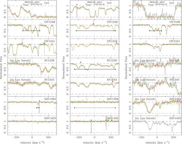
Figure 2. Normalized spectra around the Lyα, C iv, N v, and Si iv absorption lines of intrinsic systems at vshift = 37,037 km s−1 (left), 4129 km s−1 (middle), and 65,181 km s−1 (right) in the spectrum of HE0130−4021. The velocity scale is relative to the flux-weighted center of a line, calculated by Equation (4) of Misawa et al. (2007a). The first to sixth epoch spectra are shown with black, red, green, blue, light-blue, and purple histograms, respectively. Wavelength regions used for EW measurements are marked with solid arrows. If lines are not detected with >5σ level, upper limits of EWs are measured for the regions with dashed arrows. False patterns, such as cosmic rays, bad columns, and order gaps, are marked with asterisks on the spectra.
Download figure:
Standard image High-resolution image
Figure 3. Same as Figure 2, but for the system at vshift = 18,578 km s−1 in the HE0940−1050 spectrum.
Download figure:
Standard image High-resolution image3. MEASUREMENTS AND RESULTS
3.1. Methodology and General Results
Our initial inspection of the normalized spectra shown in Figures 2–13 did not reveal any substantial variations in the profiles of either the NALs or the mini-BALs, i.e., no changes in the profile asymmetries or the velocities of the troughs were discernible. However, changes in the strengths of the mini-BALs were quite evident. To quantify changes in line strengths, we measured the EWs of the blue components of NALs and the entire doublet regions of mini-BALs in each of the observed epochs for each transition, i.e., C iv, Si iv, and N v. We list these measurements in Table 3 along with their uncertainties. For the mini-BALs, the doublet members often suffer self-blending and cannot be reliably separated. We calculated the 1σ error bar on the measured EW, σEW, as the sum of contributions from uncertainties in the intensities of individual pixels in the spectrum and from uncertainties in the placement of the continuum:  . The first term was evaluated by summing in quadrature the EW error bars from the N individual pixels making up the absorption trough (see horizontal arrows in Figures 2–13)
where σi is the error in the normalized intensity at pixel i and Δλi is the width of that pixel (in Å). To compute the uncertainty resulting from the continuum placement, we assumed that it is proportional to the product of the width of the line near the continuum level, λmax − λmin (see horizontal arrows in Figures 2–13), and the characteristic uncertainty of the continuum next to the line, σf. In other words, we supposed that the fitted continuum level in the spectrum could fluctuate by an amount of the order of ±σf, sweeping out an area of the order of ±(λmax − λmin)σf, which sets σcont. The fluctuations in the normalized continuum level are σf/f, where f is the observed flux density, which is the inverse of the S/N. Hence, we may write
In the above expression, we have included a "calibration parameter," A, whose value we found empirically as follows. We carried out several experiments in which we fitted the continuum around some NALs and mini-BALs multiple times, choosing different regions around them each time, so as to determine the amount by which the fitted level could fluctuate. We then compared the variation in EW measured after different continuum fits to that given by Equation (2) and found that A ≈ 0.5 very uniformly (see Figure 1). Thus we adopted Equation (2) with A = 0.5 as an estimate of the EW uncertainty resulting from continuum placement errors. We find that the continuum placement errors are the dominant source of uncertainty in the measured EWs.
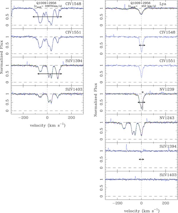
Figure 4. Same as Figure 2, but for the systems at vshift = 33,879 km s−1 (left) and 452 km s−1 (right) in the Q1009+2956 spectrum.
Download figure:
Standard image High-resolution image
Figure 5. Same as Figure 2, but for the systems at vshift = 767 km s−1 (left) and 452 km s−1 (right) in the HS1700+6416 spectrum.
Download figure:
Standard image High-resolution image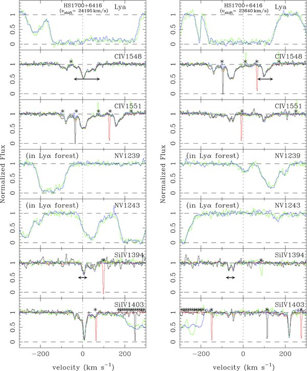
Figure 6. Same as Figure 2, but for the systems at vshift = 24,195 km s−1 (left) and 23,640 km s−1 (right) in the HS1700+6416 spectrum.
Download figure:
Standard image High-resolution image
Figure 7. Same as Figure 2, but for the systems at vshift = 927 km s−1 (left) and 96 km s−1 (right) in the HS1946+7658 spectrum.
Download figure:
Standard image High-resolution imageTo assess the significance of observed variations in the EW we computed the change in EW between two epochs as ΔEW = EW2 − EW1 (where Epoch 1 is earlier than Epoch 2) and its uncertainty as  and defined the variation significance as

Significant variability is seen preferentially in the mini-BAL systems (see Figures 14–19), but not in NALs. The greatest changes for NALs are seen from E1 → E2 of N v in the vshift ∼ 452 km s−1 system of Q1009+2956 and from E2 → E4 of N v in the vshift ∼ 767 km s−1 system of HS1700+6416. In both of these cases, the variation significance is between 1.5σ and 2σ, and this is consistent with expectations in a sample of this size that does not experience variability. It is also consistent with variations in the EWs of intervening NALs caused by measurement errors. We tabulate the measured variation significance for mini-BALs in Table 4 for the shortest time intervals where a variation was detected (in the case of Q2343+125 we only detect variability at a significance level of <2σ but we include this object in the table for completeness). Distributions of absolute variation significance, |SEW|, as a function of EW and time interval are shown in Figures 20–23 for NALs and mini-BALs, respectively. Histograms of |SEW|, measured for all unique pairs of observing epochs, are also shown in Figures 24 and 25.
Five of the six mini-BAL systems in our sample show significant variability at greater than |SEW| > 2 in at least one transition (in the sixth quasar, Q2343+125, the C iv line varied at |SEW| < 2; see Table 4). Out of 52 unique pairs of epochs plotted in the histogram of Figure 25, four are in the range 3 < |SEW| < 5 while another 6 are in the range |SEW| > 5. For NALs, we compare our sample with intervening NALs that are detected in the same spectra but are classified as intervening NALs with coverage fractions of unity (Misawa et al. 2007a). In Figure 24, we compare the distribution of |SEW| of intrinsic NALs to that of intervening NALs. This comparison shows the two distributions to be very similar and reinforces our conclusion that none of the intrinsic NALs in our sample have varied significantly.
In Figure 26, we plot the change in EW of mini-BALs for every unique pair of observing epochs, |ΔEW|, as a function of the rest-frame time interval, Δtrest. The EW changes are larger for longer time intervals for lines from all observed ions, C iv, N v, and Si iv. The trend persists if we normalize the EW changes by the average EW as shown in Figure 27. In other words, both the absolute and the fractional change in EW increase over longer time intervals (fractional variations of 50% or more occur on time intervals of a year or longer). Such a behavior has been noted for C iv BALs (Gibson et al. 2008; Capellupo et al. 2011, 2013; Filiz Ak et al. 2013). We find an analogous result, namely, when we detect significant variability in two transitions at the same time in the same system the EWs change in the same direction. We illustrate this behavior in Figure 28 where we plot the change in the Si iv or N v EW against that of C iv (see caption for error bars and other specific information). It is noteworthy, however, that we have never observed these three strong lines vary at the same time because one of them is either saturated or not detected. By comparing the data points in this figure with the straight line of unit slope included for reference, we conclude that the fractional variations of EW of lines in the same system are not necessarily proportional to each other.
If we assume that the observed changes in EW result from changes in the ionization state of the gas (see discussion in Section 1), we can set a lower limit to the electron density by taking the variability timescale, Δtrest, to be an upper limit to the recombination time of the relevant ion, i.e., ne ≳ (α Δtrest)−1, where ne is the electron density and α is the recombination coefficient of the transition in question. We use the recombination coefficients for a gas temperature of 20,000 K (Arnaud & Rothenflug 1985; Hamann et al. 1995). It is not straightforward to infer a density from recombination to/from Si iv (Arnaud & Rothenflug 1985), therefore we perform the calculations only for C iv and N v. If the EWs have increased, we assume that C v → C iv and N vi → N v, while if the EWs have decreased, we assume that C iv → C iii and N v → N iv, based on the following argument. In all cases (with a single exception; see previous paragraph) of variable mini-BAL systems, absorption lines from all ions (i.e., Si iv, C iv, and N v, with ionization potentials of 45.1, 64.5, and 97.9 eV, respectively) get stronger and weaker together. In order for all three lines to increase and decrease together, the ionization parameter should be either log U ≲ −2.5 or log U ≳ −1.5 (Hamann 1997). The regime of low U can be rejected because we do not detect any absorption lines from low ionization species with ionization potentials between 14 and 33 eV corresponding to any mini-BAL systems (e.g., O i λ1302, Fe ii λ2344, Fe ii λ2383, Si ii λ1260, Si ii λ1527, Al ii λ1671, C ii λ1335, Al iii λ1855, Al iii λ1863, and Si iii). This suggests that log U ≳ −1.5 and that as the ionization parameter varies, the main ionization states of silicon, carbon, and nitrogen vary as follows: Si iv  Si v, C iv
  C v, and N v
  N vi. Under these conditions, we estimate lower limits on the electron density in the range 1.7 × 10³–4.0 × 105 cm−3. We are only able to derive such limits for mini-BALs; since the NALs in our sample did not show significant variability, we are not able to apply this method to them. We list the results for individual objects in Table 4 and discuss them in more detail in Section 3.2
From the lower limits on the density of the mini-BAL gas, we then estimate upper limits to the distance of the absorber from the source of ionizing radiation by making use of the definition of the ionization parameter as the ratio of ionizing photon density to hydrogen number density at the illuminated face of the cloud:
where Q(H) is the emission rate of hydrogen-ionizing photons by the central engine and r is the distance of the absorber from that source. We assume that log U > − 1.5 so that C iv is the dominant ionization stage of carbon (Hamann et al. 1995, 1997b) and to satisfy the constraint that all the observed absorption lines increase and decrease together. We also assume that ne ∼ nH. Thus, we obtain Q(H) by scaling the bolometric luminosity, which we compute via Lbol = 4.4 λLλ at λ = 1450 Å, based on the spectral energy distribution (SED) of Richards et al. (2006). This SED is a segmented power law of the form Lλ∝λα with α = −1.6 from 1000 Å to 10 μm, α = −0.4 from 10 to 1000 Å, and α = −1.1 from 0.1 to 10 Å, following Zheng et al. (1997) and Telfer et al. (2002). By integrating this SED, we find that Q(H) = 1058.2 s−1 for a quasar with a bolometric luminosity of 1048 erg s−1. Inserting the expression for Q(H) and limits on ne and log U into Equation (4) and rearranging, we arrive at the following expression for the distance of the absorber from the continuum source:

where L48 is the bolometric luminosity in units of 1048 erg s−1 and n5 is the electron density in units of 105 cm−3. Using Equation (5), we estimate upper limits on the distance of the absorber to be in the range 3–6 kpc (see Table 4 and Section 3.2). These values decrease by a factor of ∼4 if we use the SED of a typical radio-loud quasar (Mathews & Ferland 1987) or a high luminosity radio-quiet quasar (Dunn et al. 2010).

Figure 8. Same as Figure 2, but for the system at vshift ∼ 1900 km s−1 in the UM675 spectrum. The spectrum is resampled every 0.3 Å.
Download figure:
Standard image High-resolution image3.2. Notes on Individual Mini-BAL Systems
Here we discuss the variable mini-BALs in more detail before moving on to a general discussion about their properties and the possible causes of variability.
- UM675 (zem = 2.15), mini-BAL system at vshift ∼ 1900 km s−1 (zabs ∼ 2.13).Time variability of the C iv and N v doublets over ⩽2.9 yr in the quasar rest frame was discovered in the mini-BAL absorber at zabs ∼ 2.13 (i.e., vshift ∼1900 km s−1) in this radio-quiet quasar (Hamann et al. 1995). Additional observations indicated that the different ions can have different coverage fractions: Cf ∼ 0.45 for C iv, Cf ⩾ 0.83 for Lyα, and Cf ⩾ 0.6 for O vi (Hamann et al. 1997b).We collected two spectra taken with Keck/HIRES and Subaru/HDS in 1994 and 2005, respectively. As shown in Figure 8, N v and C iv got weaker at a >5σ significance over ∼3.5 yr in the quasar rest frame. Lyα also showed the same trend. The variation occurs across the entire profile, though perhaps fractionally less in the central narrower component, as seen in the spectrum of Q2343+125 (Hamann et al. 1997a). We cannot distinguish between a change in ionization and a change in coverage fraction as the cause of the variability.Summary. The C iv and N v profiles have weakened on timescales of several years in the quasar rest frame. This places constraints on density (ne ⩾ 3.3 × 103 cm−3), and thus distance (r ⩽ 4.0 kpc). The detection of Ne viii (Beaver et al. 1991) also suggests proximity to the quasar, although this line is not covered by our optical spectra.
- HE0151−4326 (zem = 2.78), mini-BAL system at vshift ∼ 11,300 and 8900 km s−1 (zabs ∼ 2.64 and 2.67).This system has not yet been studied in detail as an intrinsic absorption system. There are two distinct absorption systems at vshift ∼ 8900 km s−1 (corresponding to Δv ∼ 0 – 1000 km s−1 in Figure 9) with C iv and Si iv detected, and at vshift ∼ 11,300 km s−1 (Δv ∼ −2800 to −1800 km s−1) detected in C iv. In addition to these two systems, there is likely to be a weaker system at vshift ∼ 6400 km s−1 (Δv ∼ 1500–3000 km s−1) with detected C iv.This mini-BAL system spans more than 5000 km s−1 in velocity space, although it does not satisfy the criterion for being a BAL (which requires that the observed spectrum falls at least 10% below the model of continuum plus emission lines over a contiguous velocity interval of at least 2000 km s−1).The first three epochs of observation are within one month, and neither C iv nor Si iv showed variation in EW at >5σ level, except for E2 → E3 of C iv for the vshift ∼ 8900 km s−1 system. The last epoch is separated from those first three by ∼2 yr in the quasar rest frame. The absorption is significantly stronger in the last epoch, again over the entire velocity range of observation. The Si iv is either not detected or very weak in the first three epochs, but then has appeared by the fourth epoch of observation in the component at Δv ∼ 800 km s−1 (see Figure 9). This suggests that there has been an ionization change in this component at least, and not just a change in coverage fraction. To adequately test this hypothesis, we would need high quality spectra covering some higher ionization ions such as N v and O vi.Summary. The C iv profile for this absorption complex, which spans ∼5000 km s−1, has increased in strength between observations separate by ∼2 yr in the quasar rest frame. Si iv has also appeared in one component. This is consistent with a lower degree of ionization at the later time, and places constraints on densities (ne ⩾ 3.9 × 103 cm−3), and thus distances (r ⩽ 6.3 kpc) for the vshift ∼ 11,300 km s−1 and 8900 km s−1 systems.
- Q1157+014 (zem = 2.00), mini-BAL system at vshift ∼ 3000 km s−1 (zabs ∼ 1.97).Wright et al. (1979) first studied the spectrum of this quasar in detail, and noted that it has C iv and C iii] emission lines (although the Lyα emission line is absent or extremely weak) and several BALs such as Lyα, N v, and C iv. This system is classified as a BAL by the traditional definition because of the broad absorption profiles of C iv and N v. However, we regard it as a mini-BAL in this study because Si iv is not so strong as in typical BALs.We collected five epochs of observations with VLT/UVES from 2000 to 2007, covering C iv, Si iv, and N v at multiple epochs. The profiles are shown in Figure 10. The Si iv varies significantly on a timescale of ⩽223 days (⩽80 days in the quasar rest frame). The N v appears to get a bit weaker and the C iv to get a bit stronger over the interval, but the change is at less than a 5σ level except for E1 → E4 for C iv. The C iv and N v are clearly saturated over most of the profile, and so are not subject to variations in column density. A variation in coverage fraction would lead to a significant change in those EWs, since non-unity coverage fraction would cause these saturated profiles not to be black. Thus the lack of variability in the saturated C iv and N v suggests that an ionization change is responsible for the variability of the Si iv profile in this system.Summary. This system shows variability, but mostly in the weaker Si iv absorption, and not in the saturated C iv and N v. The most plausible explanation for this is that the coverage fraction remains similar, but that the ionization state changes, because a change in the C iv and N v column density won't make a significant difference in the profile if it is saturated (e.g., Capellupo et al. 2012). This would be consistent with these profiles having changed only in their unsaturated parts. Any strict constraints cannot be placed on density and distance because recombination from/to Si iv is not simple.
- HE1341−1020 (zem = 2.134), mini-BAL system at vshift ∼ 1300 km s−1 (zabs ∼ 2.12).We found this mini-BAL system with broad absorption features of C iv and N v in the catalog of Narayanan et al. (2007). As far as we know, this system has not been previously studied in detail as an intrinsic absorption system.We collected two epochs of observations with VLT/UVES in 2001 and 2007, which are shown in Figure 11. With the two available epochs we find that both lines show time variability on a timescale of ∼2 yr in the quasar rest frame. Both the C iv and the N v are stronger at the later epoch at more than 5σ significance level, and they are stronger over the entire profile. Si iv is not detected at either epoch. The profiles again have the appearance of narrower profiles superimposed on broad ones.Summary. The C iv and N v profiles have varied on a timescale of ∼2 yr in the quasar rest frame, with both ions becoming stronger over the full range in velocity. This is certainly consistent with a change in coverage fraction, but an ionization change also cannot be ruled out with only two ions available as constraints. If an ionization change is the cause of variability, we can place constraints on density (ne ⩾ 3.0 × 103 cm−3), and distance (r ⩽ 3.5 kpc). The absorption profiles show narrow components superimposed on broader ones.
- HS1603+3820 (zem = 2.542), mini-BAL system at vshift ∼ 9500 km s−1 (zabs ∼ 2.43).This system was first discovered by Dobrzycki et al. (1999), and then monitored with high-resolution spectra for ∼1.2 yr in the quasar rest frame (Misawa et al. 2005, 2007b). The C iv mini-BAL shows both partial coverage (Misawa et al. 2003) and time variability (Misawa et al. 2005, 2007b). The C iv profile changes across the entire range of velocity, ∼2000 km s−1, at once (see Figure 12). Among three possible scenarios for the variation, (1) a gas motion, (2) a variable scattering material, and (3) a change of ionization condition, the first two cannot be applicable for this quasar (see Section 1). The preferred explanation of changing ionization parameter is likely to be caused by variable shielding material between the continuum source and the absorber, since a quasar of this luminosity does not vary enough to explain the change. Warm absorbers are a candidate for the shielding material as evidenced by X-ray observations of this quasar (Misawa et al. 2010; Rozanska et al. 2013).Summary. There is significant variability of C iv over the full velocity range on timescales as short as months in the quasar rest frame. The variability is likely to be caused by changing ionization parameter due to variable shielding material that modulates the quasar flux. We place constraints on the electron density (ne ⩾ 1.6 × 104 cm−3) and the absorber's distance from the flux source (r ⩽ 4.0 kpc).
- Q2343+125 (zem = 2.515), mini-BAL system at vshift ∼ 24, 400 km s−1 (zabs ∼ 2.24).Previously, Hamann et al. (1997a) detected C iv, N v, and Si iv mini-BALs at zabs ∼ 2.24 (corresponding to vshift ∼ 24,400 km s−1) in this radio-quiet quasar spectrum. These lines showed both time variability (the lines weakened and then strengthened again by a factor of ∼4 on a timescale of ⩽0.3 yr in the quasar rest frame) and partial coverage (Cf ⩽ 0.2 for C iv).We collected additional spectra with VLT/UVES at three different epochs from 2002 to 2007. Because of the different wavelength coverage of the different observations, only C iv has multiple observations (Figure 13). Lyα and N v are blended with the Lyα forest. The EW measurements for C iv 1548 were 3.29 ± 0.69 Å, 2.04 ± 0.44 Å, and 2.69 ± 0.63 Å for observations 1, 2, and 3, respectively, indicating only negligible variability at less than the 2σ level. We do not detect any Si iv features, while Hamann et al. (1997a) found a weak Si iv mini-BAL. Several narrow components inside the broader absorption profiles of C iv (Hamann et al. 1997a) are not apparent in our lower-S/N spectra.Summary. In this vshift ∼ 24,400 km s−1 mini-BAL, C iv gets slightly weaker, and then stronger, with changes taking place in only 124 and 403 days in the quasar rest frame, but in < 2σ level. More detailed analysis is not possible due to there being multiple epoch observations only of C iv.
4. DISCUSSION
4.1. Comparison of BAL and Mini-BAL Variability and Assessment of Physical Mechanisms
The observational results of our monitoring campaign, combined with earlier case studies (e.g., Misawa et al. 2007b; Hamann et al. 2011; Rodríguez Hidalgo et al. 2012 and references therein), suggest some similarities between the variability patterns observed in mini-BALs and BALs. In particular, we have found that the EWs of all mini-BALs in our sample vary on rest-frame timescales of months to years and have observed the following patterns (1) when different transitions in a mini-BAL system vary together, their EWs change in the same direction, (2) absolute and relative changes in EWs are larger over longer rest-frame time intervals, and (3) variations in the EWs of the lines are not accompanied by discernible changes in the profiles, i.e., different troughs in the profile vary together. In comparison (1) more than 50% of BALs vary over timescales of the order of a year in the quasar rest-frame with the probability of variation approaching unity on multi-year timescales (e.g., Capellupo et al. 2011, 2013), and (2) the EWs of the UV absorption lines from C iv, Si iv, and N v in BAL systems vary together and in the same direction, although not necessarily in proportion to each other (e.g., Filiz Ak et al. 2013). However, BAL profiles do vary as the EWs vary (e.g., Lundgren et al. 2007; Gibson et al. 2008; Capellupo et al. 2011; Filiz Ak et al. 2012, 2013) in contrast to what is observed for mini-BAL troughs. In view of the similarities, we consider the two variability mechanisms often discussed for BALs as explanations for the observed mini-BAL variability, gas motion across our sightline and change of ionization conditions (see Section 1 for references and more details)

Figure 9. Same as Figure 2, but for the system at vshift ∼ 11,300 km s−1 and 8900 km s−1 in the HE0151−4326 spectrum. The spectrum is resampled every 0.3 Å.
Download figure:
Standard image High-resolution image
Figure 10. Same as Figure 2, but for the system in the vshift ∼ 3000 km s−1 of Q1157+014 spectrum. The spectrum is resampled every 0.3 Å.
Download figure:
Standard image High-resolution image
Figure 11. Same as Figure 2, but for the system in the vshift ∼ 1300 km s−1 of HE1341−1020 spectrum. The spectrum is resampled every 0.3 Å.
Download figure:
Standard image High-resolution image
Figure 12. Same as Figure 2, but for the system at vshift ∼ 9500 km s−1 in the HS1603+3820 spectrum. The spectrum is resampled every 0.3 Å.
Download figure:
Standard image High-resolution image
Figure 13. Same as Figure 2, but for the system at vshift ∼ 24,400 km s−1 in the Q2343+125 spectrum. The spectrum is resampled every 0.3 Å.
Download figure:
Standard image High-resolution image
Figure 14. Monitoring results for EWs of C iv (red), N v (green), and Si iv (blue) lines in the mini-BAL at vshift ∼ 1900 km s−1 in the UM675 spectra. The horizontal axis is the time delay from the first epoch in the quasar rest frame (in years). The vertical axis is the observed EW (with 1σ errors) normalized to that of the first observed epoch. If the observed spectrum does not cover a particular line, that epoch is not plotted for that line. If lines are covered but not detected, upper limits are marked with downward arrows.
Download figure:
Standard image High-resolution imageTable 3. Observed Frame Equivalent Width
| EWobs | ||||||
|---|---|---|---|---|---|---|
| QSO | vshift | Epoch | Δta | N v | Si iv | C iv |
| (km s−1) | (days) | (Å) | (Å) | (Å) | ||
| (1) | (2) | (3) | (4) | (5) | (6) | (7) |
| HE0130−4021 | 65181 | 1 | 0 | b | b | 0.99 ± 0.05 |
| 2 | 2573 | b | b | 0.99 ± 0.07 | ||
| 3 | 4269 | b | b | 1.017 ± 0.04 | ||
| 37037 | 1 | 0 | b | 0.057 ± 0.008f | 1.49 ± 0.08 | |
| 2 | 2573 | b | 0.059 ± 0.013 | 1.46 ± 0.12 | ||
| 3 | 4269 | b | 0.054 ± 0.007 | 1.45 ± 0.07 | ||
| 4129 | 1 | 0 | 1.87 ± 0.14 | <0.23 | - | |
| 2 | 2573 | 1.82 ± 0.18 | <0.28 | 1.17 ± 0.25f | ||
| 3 | 4269 | 1.73 ± 0.11f | <0.17 | 1.15 ± 0.15 | ||
| HE0940−1050 | 18578 | 1 | 0 | - | 0.538 ± 0.028 | 1.62 ± 0.06 |
| 2 | 311 | b | 0.533 ± 0.014 | 1.65 ± 0.03 | ||
| 3 | 2620 | b | 0.542 ± 0.021 | 1.61 ± 0.05 | ||
| Q1009+2956 | 33879 | 1 | 0 | - | 0.900 ± 0.030 | 1.73 ± 0.03 |
| 2 | 1082 | - | 0.908 ± 0.003 | - | ||
| 3 | 1166 | - | 0.895 ± 0.014 | - | ||
| 4 | 4176 | - | 0.926 ± 0.048 | 1.72 ± 0.06 | ||
| 452 | 1 | 0 | 0.434 ± 0.008f | 0.019 ± 0.014 | - | |
| 2 | 1082 | 0.392 ± 0.005 | - | - | ||
| 3 | 1166 | 0.405 ± 0.004 | - | - | ||
| 4 | 4176 | 0.399 ± 0.016 | 0.018 ± 0.009 | 0.430 ± 0.015 | ||
| HS1700+6416 | 24195 | 1 | 0 | - | 0.102 ± 0.019 | 0.406 ± 0.033 |
| 2 | 398 | - | 0.104 ± 0.006 | 0.424 ± 0.014 | ||
| 3 | 4109 | b | 0.084 ± 0.015 | 0.430 ± 0.036f | ||
| 4 | 4152 | b | 0.106 ± 0.01 | 0.417 ± 0.027 | ||
| 23640 | 1 | 0 | - | 0.087 ± 0.017 | 0.196 ± 0.019f | |
| 2 | 398 | - | 0.100 ± 0.007 | 0.216 ± 0.007f | ||
| 3 | 4109 | b | 0.085 ± 0.015 | 0.189 ± 0.018f | ||
| 4 | 4152 | b | 0.089 ± 0.014 | 0.197 ± 0.012 | ||
| 767 | 1 | 0 | 0.501 ± 0.027 | <0.02 | 0.291 ± 0.016 | |
| 2 | 398 | 0.465 ± 0.009 | <0.007 | 0.295 ± 0.007 | ||
| 3 | 4109 | 0.500 ± 0.031 | <0.02 | 0.328 ± 0.021 | ||
| 4 | 4152 | 0.504 ± 0.022 | <0.01 | 0.318 ± 0.015 | ||
| 452 | 1 | 0 | 0.108 ± 0.015 | <0.015 | <0.011 | |
| 2 | 398 | 0.101 ± 0.006 | <0.006 | <0.005 | ||
| 3 | 4109 | 0.084 ± 0.015 | <0.02 | <0.02 | ||
| 4 | 4152 | 0.109 ± 0.012 | <0.01 | <0.01 | ||
| HS1946+7658 | 927 | 1 | 0 | <0.01 | <0.01 | 0.286 ± 0.007 |
| 2 | 1517 | <0.01 | - | - | ||
| 3 | 1549 | <0.01 | - | - | ||
| 96 | 1 | 0 | 0.366 ± 0.008 | 2.318 ± 0.01 | 4.164 ± 0.02 | |
| 2 | 1517 | 0.384 ± 0.014 | - | - | ||
| 3 | 1549 | 0.371 ± 0.012 | - | - | ||
| UM675 | ∼1900 | 1 | 0 | 6.15 ± 1.01 | <0.4 | 5.38 ± 0.24 |
| 2 | 3982 | 3.63 ± 0.33 | <0.3 | 3.84 ± 0.21 | ||
| HE0151−4326 | ∼11300 | 1 | 0 | b | <0.07 | 1.96 ± 0.26 |
| 2 | 19 | - | <0.10 | 2.12 ± 0.37 | ||
| 3 | 58 | b | <0.10 | 2.22 ± 0.36 | ||
| 4 | 2176 | b | 0.24 ± 0.16 | 3.69 ± 0.53 | ||
| ∼8900 | 1 | 0 | b | 0.09 ± 0.04 | 4.07 ± 0.21 | |
| 2 | 19 | - | 0.10 ± 0.06 | 4.22 ± 0.30 | ||
| 3 | 58 | b | 0.08 ± 0.06 | 3.92 ± 0.32 | ||
| 4 | 2176 | - | 0.59 ± 0.09 | 10.42 ± 0.43 | ||
| Q1157+014 | ∼3000 | 1 | 0 | 38.38 ± 1.28 | - | 37.12 ± 1.23 |
| 2 | 410 | 38.27 ± 1.17 | 9.16 ± 0.52c | - | ||
| 3 | 633 | - | 10.31 ± 1.23c | - | ||
| 4 | 2094 | 37.7 ± 4.5 | 9.77 ± 1.12c | 38.17 ± 2.33 | ||
| 5 | 2593 | - | 11.26 ± 0.71c | 38.53 ± 1.05 | ||
| HE1341−1020 | ∼1300 | 1 | 0 | 15.39 ± 0.47 | <0.3 | 6.86 ± 0.24 |
| 2 | 2280 | 21.63 ± 0.79 | <0.7 | 12.40 ± 0.45 | ||
| HS1603+3820 | ∼9500 | 1 | 0 | - | - | 10.12 ± 1.15 |
| 2 | 471 | b | d | 17.95 ± 1.84 | ||
| 3 | 1071 | b | <0.8e | 13.62 ± 0.79 | ||
| 4 | 1194 | b | d | 13.03 ± 1.43 | ||
| 5 | 1245 | b | d | 12.69 ± 0.84 | ||
| 6 | 1530 | - | <0.5 | 13.34 ± 0.61 | ||
| Q2343+125 | ∼24400 | 1 | 0 | - | - | 3.29 ± 0.69 |
| 2 | 437 | b | - | 2.04 ± 0.44 | ||
| 3 | 1855 | - | <0.76 | 2.69 ± 0.63 | ||
Notes. aTime delay from the first epoch in the observed frame. bThis line is blended with the Lyα forest. cParameters are measured using only blue component, because doublet lines are not self-blended and can be fitted separately. dThis line is significantly affected by bad columns. eSpectral region is partially truncated. fThis line is affected by a data defect that could slightly alter the EW measurement. − This line is not covered by the observed spectrum.
To evaluate the likelihood that the mini-BAL variations result from motion of the absorbing gas across the line of sight, we estimate the timescale for a parcel of gas to cross the cylinder of sight that encompasses either the continuum source or the BLR. We take the transverse speed of the absorber to be of the same order as the observed outflow speed (both are related to the free-fall speed, the only velocity scale in the problem), i.e., v ∼ 104 km s−1. We assume that the observed UV continuum is emitted from the inner parts of the accretion disk within a radius acont ∼ 10 rg from the center, where rg ≡ GM•/c2 is the gravitational radius and M• is the mass of the black hole, i.e., acont ∼ 1.5 × 10¹⁵ M9 cm, where M9 = M•/109 M☉. Using the bolometric luminosities from Table 4 and assuming that the accretion rates are close to the Eddington limit, we estimate the black hole masses to be in the range: M9 = 2–15, which leads to continuum source radii in the range acont ∼ 3 × 10¹⁵–2.3 × 1016 cm and crossing times tcross(acont) ∼ 0.09–0.7 yr. For the radius of the BLR, we adopt the relation between it and the continuum luminosity given by Kaspi et al. (2007), which leads to aBLR ∼ 0.22–0.63 pc and crossing times of tcross(aBLR) ∼ 20–60 yr. The long crossing times of the BLR lead us to disfavor gas motion across the BLR cylinder of sight as the cause of variability. Moreover, a substantial fraction of the mini-BAL troughs in our sample are found at large outflow velocities, |vshift| ≳ 5000 km s−1, so that they do not overlap with the broad emission lines (i.e., the mini-BAL gas absorbs only continuum photons and the continuum source crossing time is the more relevant timescale). These considerations make this particular version of the scenario very unlikely. The crossing times of the continuum source for the more luminous quasars in our sample are on a par with the observed variability timescales and the amplitude of EW variations is largest for timescales just over a year, which is comparable to the time required to traverse the continuum source completely. However, for the less luminous quasars in our sample, we would have expected the EW variations to be faster. Moreover, all troughs in a mini-BAL system vary together when the EW varies, which is difficult to orchestrate unless the parcels of gas producing the mini-BAL troughs in a given system all cross the cylinder of sight to the continuum source at the same time. Thus, we disfavor this version of the scenario as the cause of variability, although we cannot decisively rule it out (see also the discussion in Rodríguez Hidalgo et al. 2011).
As argued by Misawa et al. (2007b), the fact that all troughs in a mini-BAL system vary together strongly suggests that the variability is the result of changes in the ionization state of the absorber, presumably because of a variable ionizing continuum. Filiz Ak et al. (2014) suggest that this mechanism may also operate in BALs. But since the continuum variability timescales of such luminous quasars are considerably longer than the observed variability of mini-BALs (e.g., Giveon et al. 1999; Hawkins 2001; Kaspi et al. 2007), one is led to invoke variable obscuration of the ionizing continuum seen by the absorbers by shielding material of variable column density. This screen could be the X-ray warm absorber (Gallagher et al. 2002, 2006), and indeed some X-ray absorbers toward mini-BAL quasars show this particular behavior (e.g., Giustini et al. 2011). In this scenario, an X-ray warm absorber lies along sight lines toward mini-BAL and BAL systems but not toward NAL absorbers. This conclusion is based on the measurement of high column densities from the X-ray spectra of quasars with BALs and mini-BALs but not from the spectra of quasars with intrinsic NALs (e.g., Chartas et al. 2009). Recent radiation-MHD simulations by Takeuchi et al. (2013) reproduce variable clumpy structures in warm absorbers with typical sizes or order 20 rg and typical optical depth of the order of unity. They appear above heights of ∼500 rg from the plane of the accretion disk but, interestingly, they are not found at very high latitudes, where sight lines towards intrinsic NAL absorbers have been suggested to be by Ganguly et al. (2001) and Misawa et al. (2008). The fact that these clumps have sizes comparable to the size of the continuum source, suggests that they can modulate the apparent size of the continuum source and, by extension, the coverage fraction of the absorbers. Thus, such clumpy structures provide a plausible explanation for the frequent variability of mini-BALs and the lack of frequent variability in intrinsic NALs.

Figure 15. Same as Figure 14, but for a mini-BAL at vshift ∼ 11,300 km s−1 (top) and 8900 km s−1 (bottom) in the spectra of HE0151−4326.
Download figure:
Standard image High-resolution image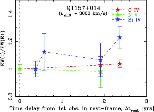
Figure 16. Same as Figure 14, but for a mini-BAL at vshift ∼ 3000 km s−1 in the spectra of Q1157+014.
Download figure:
Standard image High-resolution image
Figure 17. Same as Figure 14, but for a mini-BAL at vshift ∼ 1300 km s−1 in the spectra of HE1341−1020.
Download figure:
Standard image High-resolution image
Figure 18. Same as Figure 14, but for a mini-BAL at vshift ∼ 9500 km s−1 in the spectra of HS1603+3820.
Download figure:
Standard image High-resolution image
Figure 19. Same as Figure 14, but for a mini-BAL at vshift ∼ 24,400 km s−1 in the spectra of Q2343+125.
Download figure:
Standard image High-resolution image
Figure 20. Variation significance, |SEW| ≡ |ΔEW|/σΔEW (see Equation (3)), as a function of the average, rest-frame EW for NALs. Intrinsic C iv, N v, and Si iv NALs are marked with red, green, and blue stars, while intervening NALs with full coverage are marked with crosses and included for comparison.
Download figure:
Standard image High-resolution image
Figure 21. Same as Figure 20, but for mini-BALs. The |SEW| = 3 and 5 thresholds are marked with horizontal dotted lines.
Download figure:
Standard image High-resolution image
Figure 22. Variation significance, |SEW| ≡ |ΔEW|/σΔEW (see Equation (3)), as a function of time interval for NALs. Intrinsic C iv, N v, and Si iv NALs are marked with red, green, and blue stars, while intervening NALs with full coverage are marked with crosses for comparison.
Download figure:
Standard image High-resolution image
Figure 23. Same as Figure 22, but for mini-BALs. The |SEW| = 3 and 5 thresholds are marked with horizontal dotted lines.
Download figure:
Standard image High-resolution image
Figure 24. Distribution of variation significance, |SEW| ≡ |ΔEW|/σΔEW (see Equation (3)) for intrinsic NALs (red histogram) and intervening NALs (blue histogram). We include all unique pairs of observing epochs.
Download figure:
Standard image High-resolution image4.2. Variability of NALs and Narrow Components in Mini-BAL Systems
It is noteworthy that the intrinsic NALs we have monitored in this program did not show any variability. These were identified as intrinsic systems based on the fact that their C iv, N v, or Si iv doublets show the signature of partial coverage of the background source. Although the same signature is seen on some rare occasions in low ionization lines from intervening absorbers (presumably arising in cold and compact parcels of gas; see Kobayashi et al. 2002; Jones et al. 2010; Chen & Qin 2013), it has never been seen in high-ionization lines, such as C iv and N v, from intervening absorbers. Therefore, we are confident that the systems we have targeted are intrinsic. Moreover, variability has been observed in NALs in other monitoring campaigns, both at high and low redshifts, by Narayanan et al. (2004) and Wise et al. (2004). The NAL variability timescales and resulting lower limits on electron densities from those two studies are comparable to what we have found here for mini-BALs.
Narrow kinematic components are sometimes also found near the centers of mini-BALs. Examples in our sample can be seen at vshift ∼ 24,400 km s−1 in the C iv mini-BAL of HE1341−1020, at ∼1300 km s−1 in the C iv and N v mini-BALs of UM675, and at ∼3000 km s−1 in the Si iv mini-BAL of Q1157+014. Among these, we can monitor the narrow components in UM675 without complications from noise and line blending. The narrow C iv components of UM675 in Epochs 1 and 2 are shown in Figure 29, in which broader absorption troughs are fitted out by high-order spline functions. The total EWs (including both C iv λ1548 and C iv λ1551) of Epochs 1 and 2 are measured to be EW(E1) = 0.58 ± 0.02 and EW(E2) = 0.56 ± 0.01. Thus, they show no variability over a time interval of Δtrest ∼ 3.5 yr. Hamann et al. (1997a) noted a similar behavior for the narrow core of the C iv mini-BAL in Q2343+125 and suggested the narrow components may not be physically associated to the quasar itself, but arising in the quasar host galaxy or foreground galaxy (although this quasar is one of our targets, we cannot monitor the variability of the narrow components because our spectra have lower S/N than those of Hamann et al. 1997a). However, narrow components appear to always coincide with the centers of mini-BAL profiles, which suggests a physical association between the absorbing media. One possible explanation for the behavior of the narrow cores of mini-BALs is that they originate in dense clumps of high optical depth, embedded in the mini-BAL flow. When the ionizing continuum varies, the broad mini-BAL troughs show an easily discernible response but the highly saturated, narrow cores do not.

Figure 25. Same as Figure 24, but for mini-BALs. The |SEW| = 3 and 5 thresholds are marked with vertical dotted lines.
Download figure:
Standard image High-resolution imageTable 4. Variability and Physical Properties of Mini-BAL Absorbers
| QSO | vshift | tvara | SEWb | Ion | Ionization | Lbolc | ned | re |
|---|---|---|---|---|---|---|---|---|
| (km s−1) | (days) | Change | (erg s−1) | (cm−3) | (kpc) | |||
| (1) | (2) | (3) | (4) | (5) | (6) | (7) | (8) | (9) |
| UM675 | ∼1900 | 3982 (E1 → E2) | −2.4 | N v | N v → N iv | 3.8 × 1047 | ⩾1.66 × 10³ | ⩽5.6 |
| −4.8 | C iv | C iv → C iii | ⩾3.27 × 10³ | ⩽4.0 | ||||
| HE0151−4326 | ∼11300 | 2118 (E3 → E4) | +2.3 | C iv | C v → C iv | 1.1 × 1048 | ⩾3.90 × 10³ | ⩽6.3 |
| ∼8900 | 2118 (E3 → E4) | +4.9 | Si iv | Si v → Si iv | g | g | ||
| ∼8900 | 2118 (E3 → E4) | +12.2 | C iv | C v → C iv | ⩾3.90 × 10³ | ⩽6.3 | ||
| Q1157+014 | ∼3000 | 2183 (E2 → E5) | +2.4 | Si iv | Si v → Si iv | 2.9 × 1047 | f | f |
| HE1341−1020 | ∼1300 | 2280 (E1 → E2) | +6.8 | N v | N vi → N v | 2.6 × 1047 | ⩾1.75 × 10³ | ⩽4.5 |
| +10.8 | C iv | C v → C iv | ⩾3.00 × 10³ | ⩽3.5 | ||||
| HS1603+3820 | ∼9500 | 471 (E1 → E2) | +3.6 | C iv | C v → C iv | 1.9 × 1048 | ⩾1.64 × 10⁴ | ⩽4.0 |
| Q2343+125 | ∼24400 | 1855 (E1 → E3) | ⩽2.0 | C iv | C iv | 7.5 × 1047 | g | g |
Notes. aTime interval in the observed frame in units of days. We list only the shortest time intervals on which variability was detected since these yield the most stringent limit on the density of the absorbing gas (see Section 3.1). bVariation significance, defined as SEW ≡ ΔEW/σEW; see Equation (3). We have included a low-significance measurement for Q2343+125 for completeness since we have not detected more significant variability in this object. cBolometric luminosity, calculated as Lbol = 4.4 λLλ(1450 Å). dElectron density, calculated by assuming that the variation timescale is the recombination time. eAbsorber's distance from the flux source, calculated by assuming the quasi-static photoionization change. These numbers become smaller by a factor of ∼4 if we use the SED of typical radio-loud quasar (Mathews & Ferland 1987) or high luminosity radio-quiet quasars (Dunn et al. 2010). fNo constraints can be placed because recombination processes to/from Si iv do not lead to constraints on the density in straightforward way (Arnaud & Rothenflug 1985). gNo constraints can be placed because of no time variation.
Download table as: ASCIITypeset image

Figure 26. Change in the absolute rest-frame EW of mini-BALs as a function of rest-frame time interval for every unique pair of observing epochs. C iv, N v, and Si iv data are shown with red, green, and blue stars with 1σ errors, respectively. The dashed and solid curves denote upper envelopes of the distribution with and without a outlying point at |ΔEWrest| > 2 Å. They are included only as a guide to the eye. The outlying point corresponds to the system at vshift ∼ 9500 km s−1 in HS1603+3820 (E1 → E2). Note that the horizontal axis is logarithmic.
Download figure:
Standard image High-resolution image
Figure 27. Change in the fractional equivalent width (|ΔEW|/〈EW〉) as a function of rest-frame time interval. The vertical axis is the observed EW (with 1σ errors) normalized to the average EW in the observed-frame. The solid curve denotes an upper envelope of the distribution and is included only as a guide to the eye. The symbols have the same meaning as in Figure 26 and the horizontal axis is logarithmic.
Download figure:
Standard image High-resolution image4.3. Possible Geometry and Locations of Mini-BAL and NAL Gas
The variability properties of mini-BALs and NALs reported here, in combination with previous reports in the literature (see references above), lead us to suggest the following possibilities for locations of the absorbing gas. These are inspired by numerical simulations of quasar outflows (see references in Section 1) and are a refinement of the picture suggested by Ganguly et al. (2001).
In the first scenario, both types of absorbers are located in an accretion-disk wind, as illustrated in Figure 30. The mini-BAL gas is in the form of filaments rising from the fast component of the outflow. They make up the interface between the dense BAL wind at low latitudes above the disk and a hotter, much more tenuous medium in the polar direction. As such, the mini-BAL filaments have a large outflow speed, comparable to that of the BAL gas and a substantial velocity gradient. Within those filaments there may exist small, dense clumps that are sometimes observed as narrow cores in mini-BAL troughs. Variability of the ionizing continuum incident on the mini-BAL filaments can change the optical depth of the mini-BAL troughs arising in the filaments but not those of their narrow cores which arise in the dense clumps with C iv optical depths of τC IV ≫ 1 (assuming their predicted hydrogen column densities of ≳ 1020 cm−2, log U ∼ −1.5, and solar abundances). In this scenario, the NALs and the narrow cores of mini-BALs arise in higher-density, smaller filaments in the same region of the wind or at higher latitudes. It is possible that the NAL filaments are denser than the mini-BAL filaments thus the NALs are less susceptible to fluctuations in the ionizing continuum. However, NALs could vary because of changes in the coverage fraction, which could come about as the apparent size of the background source changes because of fluctuations in the structure of the inner screen (see discussion at the end of Section 4.3).
Alternatively, the NAL gas may be located in the host galaxy, at large distances from the center, as we noted in Section 1. In this scenario, small NAL filaments may form from the interaction of the wind's blast wave with cold clouds in the host galaxy, as proposed by Faucher-Giguère et al. (2012). Radiative shocks resulting from this interaction can create thin, dense filaments whose properties are consistent with what is inferred from photoionization models for the NAL absorbers (e.g., Wu et al. 2010; Borguet et al. 2013) and are likely to have τC IV ≫ 1. Thus the variability of the NALs arising in these filaments is more likely to result from fluctuations in the coverage fraction than fluctuations in the ionizing continuum. This scenario is more likely to apply to associated NALs, with vshift ⩽ 5000 km s−1, as this range of blueshifts better matches the prediction of numerical models for the interaction of quasar outflows with the ISM of the host galaxy (Kurosawa & Proga 2009). NALs found at vshift ≫ 5000 km s−1 (e.g., 20,000–65,000 km s−1; see Misawa et al. 2007a) are better explained by the previous scenario.
The underlying hypotheses in the above scenarios are that (1) NAL variations are more rare than those of mini-BALs (although when NALs do vary they do so on the same timescales as mini-BALs), and (2) that NAL variability is caused primarily by fluctuations in the coverage fraction while the variability of mini-BALs can be caused by fluctuations in both the coverage fraction and the ionizing continuum. Both of these hypotheses warrant further testing, which can be done by a more detailed analysis of the data we have presented in this paper as well as data collected from denser monitoring campaigns on select targets.
5. SUMMARY
We have monitored 12 intrinsic NALs (selected by their partial coverage signature) and 7 mini-BALs in quasars of zem ≈ 2–3 for ∼4–12 yr (∼1–3.5 yr in the quasar rest-frame). Using high-dispersion spectra, we have measured the line EWs as a function of time and have looked for substantial variations in the line profiles. Our main results are as follows.
- 1.We detect significant variability in the EWs of mini-BALs without any discernible changes in their profiles. However, we do not detect any significant variability in the NALs or in the narrow cores that are sometimes present in mini-BAL profiles.
- 2.The EW variability of mini-BALs is larger on longer timescales, a behavior that has also been seen in BALs.
- 3.When we are able to measure variations in the EW of more than one transition at the same time (C iv, Si iv, N v), the changes occur in the same direction. This pattern has also been observed in BALs and is consistent with a scenario in which the variations result from changes in the ionizing continuum.
- 4.If we assume that the variability timescale is the recombination time, then we can place lower limits on the electron density of the mini-BAL gas of ∼103–104 cm−2. These imply upper limits on the distances of the absorbers in the range 3–6 kpc, which could be reduced by a factor of ∼4 for a different choice of quasar SED.
- 5.The observational results lead us to suggest two possible scenarios for the structure and location of the mini-BAL and NAL gas. In the first scenario, both types of absorber are associated with the high-latitude potion of an accretion-disk wind while in the second, the NAL gas is at distances ≳ 100 pc from the quasar central engine.
The next stage of this work will entail a more detailed analysis of the variability data to study the behavior of the coverage fractions and the relative strengths of different lines, and interpret these with the help of photoionization models. Further progress in characterizing and interpreting the variability properties of mini-BALs and NALs can be made via dense monitoring campaigns of select targets in which we can observe changes on shorter timescales than we were able to probe here and associate them with changes in the ionizing continuum (via X-ray and UV observations). The data from such campaigns can also help us place better constraints on the scenario in which variability is cause by parcels of gas crossing the cylinder of sight to the continuum source.
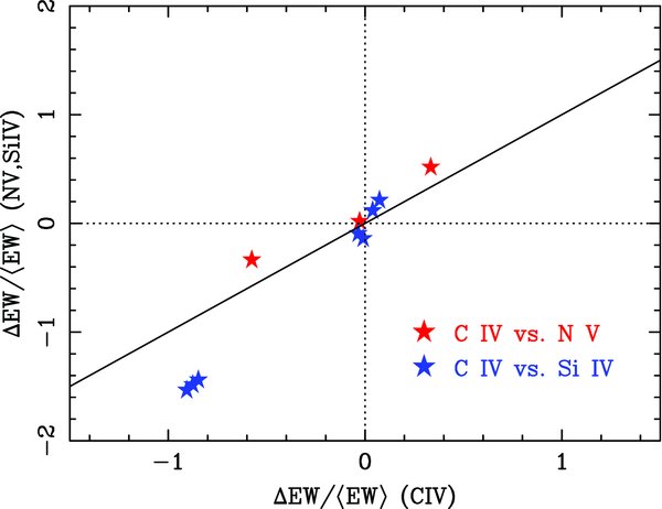
Figure 28. Fractional variations of the observed EWs of the S iv and N v mini-BALs plotted against the corresponding fractional variations of the C iv mini-BALs in the same systems. The EW error bars are not plotted as they are smaller than the size of the symbols (see Figure 26). In all but one case, different lines from the same system vary together, in the same direction. The mini-BAL of Q1157+014, marked by the red star closest to the origin, appears to be an exception (the EW of N v appears to decrease while the other two lines appear to get stronger) but the statistical significance is very low. We also plot a straight solid line with unit slope for reference.
Download figure:
Standard image High-resolution image
Figure 29. Absorption profiles of the kinematic narrow components at vshift ∼ 1900 km s−1 of the mini-BAL of UM675. The red curve corresponds to Epoch 1 and the blue curve to Epoch 2. The latter is shifted downwards by 0.1 for clarity. The broader, mini-BAL trough is removed by fitting it high order spline function. Both members of the C v λλ1548,1551 doublet are shown.
Download figure:
Standard image High-resolution image
Figure 30. Possible geometry of the locations of NAL, mini-BAL, and BAL absorbers in the accretion-disk wind scenario (see text in detail).
Download figure:
Standard image High-resolution image
It would also be extremely useful to quantify the properties that the variable shield we have invoked must have in order to produce the desired behavior. There are a number of constraints that such a shield must satisfy: it must reproduce the low column densities observed in the X-ray spectra, the continuum it transmits must lead to the observed ionization state of the UV absorber, and its structure must allow for variations in far-UV transparency and apparent source size to vary in order to reproduce the observed mini-BAL variability. It is also worth considering further different geometric arrangements of the shield, the absorber, and the background source(s) relative to the cylinder of sight, specifically whether the source of ionizing photons, the shield, and the mini-BAL gas must all be aligned.
We thank David Tytler and Fred Hamann for providing us with their Keck/HIRES data. We also thank the anonymous referee for a number of comments that helped us improve the paper. The research was supported by JGC-S Scholarship Foundation. This work was also supported by NASA grant NAG5-10817 and by NSF grants AST-0807993 and AST-1312686 at Penn State. M.E. thanks the Center for Relativistic Astrophysics at Georgia Tech and the Department of Astronomy at the University of Washington for their warm hospitality during the writing of this manuscript.
Footnotes
- *
Based on data collected at Subaru telescope, which is operated by the National Astronomical Observatory of Japan.
- †
Data presented herein were obtained at the W. M. Keck Observatory, which is operated as a scientific partnership among the California Institute of Technology, the University of California and the National Aeronautics and Space Administration. The Observatory was made possible by the generous financial support of the W. M. Keck Foundation.
- ‡
Based on observations obtained at the European Southern Observatory at La Silla, Chile in programs 65.O-0063(B), 65.O-0474(A), 67.A-0078(A), 68.A-0461(A), 69.A-0204(A), 70.B-0522(A), 072.A-0346(A), 076.A-0860(A), 079.B-0469(A), and 166.A-0106(A).
- 6
IRAF is distributed by the National Optical Astronomy Observatories, which are operated by the Association of Universities for Research in Astronomy, Inc., under cooperative agreement with the National Science Foundation.