


ABSTRACT
The interaction of comets with the solar wind has been the focus of many studies including numerical modeling. We compare the results of our multifluid MHD simulation of comet 1P/Halley to data obtained during the flyby of the European Space Agency's Giotto spacecraft in 1986. The model solves the full set of MHD equations for the individual fluids representing the solar wind protons, the cometary light and heavy ions, and the electrons. The mass loading, charge–exchange, dissociative ion–electron recombination, and collisional interactions between the fluids are taken into account. The computational domain spans over several million kilometers, and the close vicinity of the comet is resolved to the details of the magnetic cavity. The model is validated by comparison to the corresponding Giotto observations obtained by the Ion Mass Spectrometer, the Neutral Mass Spectrometer, the Giotto magnetometer experiment, and the Johnstone Plasma Analyzer instrument. The model shows the formation of the bow shock, the ion pile-up, and the diamagnetic cavity and is able to reproduce the observed temperature differences between the pick-up ion populations and the solar wind protons. We give an overview of the global interaction of the comet with the solar wind and then show the effects of the Lorentz force interaction between the different plasma populations.
Export citation and abstract BibTeX RIS
1. INTRODUCTION
The European Space Agency's Giotto spacecraft flew by comet 1P/Halley on 1986 March 14. Giotto passed roughly 600 km in front of the comet and provided a wealth of measurements (see Reinhard 1986). Several instruments observed the plasma interaction of the comet with the solar wind: ion and neutral gas abundances were measured with the Neutral Mass Spectrometer (NMS; Krankowsky et al. 1986) and the Ion Mass Spectrometer (IMS; Balsiger et al. 1986), respectively, and the magnetic field along the Giotto trajectory (Raeder et al. 1987) was observed by the Giotto magnetometer (MAG; Neubauer et al. 1986). Formisano et al. (1990) calculated the temperatures and densities of several of the observed ions from measurements with the Giotto Johnstone Plasma Analyzer instrument (JPA; Johnstone et al. 1986). All these observations revealed multiple boundaries and distinct regions in this interaction (see Altwegg et al. 1993; Häberli et al. 1995, 1996; d'Uston et al. 1987), starting from the comet's bow shock all the way to the cavity, which is the magnetic field-free region in the innermost coma (see Cravens 1989). The boundary of the diamagnetic cavity, also called the contact surface or ionopause, is located just outside the inner shock at which the cometary plasma is first entrained in the more or less radially outflowing neutral gas and then transitions from supersonic to subsonic speeds. At the contact surface, the plasma from the cometary origin merges with the mass-loaded solar wind plasma from further upstream. The nature of this interaction therefore forces the magnetic field to pile up and drape around the diamagnetic cavity, while the ionosphere inside remains field-free (Neubauer et al. 1986). Farther away from this region, the collisionopause or cometopause has been identified where cometary ions dominate the plasma density over the solar wind proton density (see Balsiger 1990) and separate the collisionless solar wind plasma flow from the cometary gas. Even farther away at the bow shock, the solar wind, which is decelerated due to the mass loading, transitions from supersonic to subsonic speeds. Given its trajectory, Giotto crossed the bow shock at roughly 1 Mkm at the flank (Rème et al. 1986).
Given the retrograde motion of comet 1P/Halley around the Sun, the fly-by happened at a large relative velocity of almost 70 km s−1 and thus only lasted a few tens of minutes. In order to extrapolate from the limited measurements to a global picture of this interaction, numerical modeling can be employed. The length scale of the interaction region of a few million kilometers compared to the size of the comet of just a few kilometers requires multiscale numerical tools. Comet Halley has been the target for various modeling studies since and even before the Giotto mission.
Some of the approaches focused on the global scale interaction or at least on part of it (e.g., Gombosi et al. 1996; Murawski et al. 1998; Baranov & Lebedev 1993), while others were dedicated to the investigation of the different species detected in the vicinity of the comet and the associated chemistry (e.g., Wegmann et al. 1987; Schmidt et al. 1988; Haider & Bhardwaj 2005; Rubin et al. 2009).
Benna & Mahaffy (2007) published their results of a multifluid global MHD model that dynamically separated neutral gas from the ions and the electrons. Similarly, in this work, we apply a global scale multifluid MHD model to investigate the cometary environment validated with the Giotto measurements of the thermal component of the plasma at 1P/Halley during the time of the fly-by. Previously, our multifluid code has been applied to other bodies in the solar system, such as Mars (Najib et al. 2011) and Earth (Glocer et al. 2009). Our model originates from the work by Gombosi et al. (1996). The major difference relative to the model by Benna & Mahaffy (2007) is that we dynamically separate the solar wind protons, cometary light ions, and heavy ions, but prescribe the neutral gas analytically. This allows us to investigate how the different plasma populations interact with each other through the Lorentz force and the collisional coupling between the species. We are also able to derive the temperatures of the different plasma populations, which is important for describing the observed temperature difference between the pick-up and solar wind plasmas. Several important processes are taken into account: mass loading due to photoionization and electron impact ionization, the interaction between the ion fluids due to the Lorentz force, and collisional coupling accounting for elastic and inelastic collisions, charge exchange, and dissociative recombination.
The first part of this article gives a quick recapitulation of the governing multifluid MHD equations. In the same section, the source terms, which describe the comet-specific interactions between the fluids, and the numerical implementation are briefly discussed. The next part of the article is devoted to the results of the model and the comparison to the corresponding measurements. We conclude with a discussion of our findings.
2. MODEL DESCRIPTION
For a more detailed study of the interaction of the comet with the solar wind and an investigation of the involved interactions between the plasma and the neutral gas, we use the Block Adaptive Tree Solar-wind Roe Upwind Scheme (BATS-R-US) component of the Space Weather Modeling Framework (SWMF) to solve the governing multifluid MHD equations (Powell et al. 1999; Tóth et al. 2005, 2012). The basis of the model described in the following section is the multifluid MHD model (Glocer et al. 2009; Najib et al. 2011) applied to the cometary environment, i.e., to comet 1P/Halley. We have furthermore included a more self-consistent calculation of the electron pressure/temperature and extended the relevant physical interactions. In the following section, we will discuss the model in more detail as well as the applicability and limitations of the chosen approach.
2.1. Modeled Species
Table 1 summarizes the plasma populations included to model the interaction of the comet with the Sun. The first fluid consists of the solar wind protons. The second and third fluids are the cometary light and heavy ions, respectively, and originate from mass loading through photoionization, electron impact ionization, and charge exchange with the neutral gas. The fourth component represents the electrons.
Table 1. Model Species with Dominant Production and Loss Processes (These can Vary Significantly with Location; in Particular, Charge–Exchange Reactions Become the Dominant Source for Cometary Light Ions in the Outer Part of the Coma; Combi et al. 1986)
| Group | Major Production Process | Major Loss Process |
|---|---|---|
| Solar wind protons | Sun |  + H2O → H2O+ + H + H2O → H2O+ + H |
| Cometary light ions (H+, H2+) | H2O + hv →  + OH + e + OH + e |
 + H2O → H2O+ + H + H2O → H2O+ + H |
| Cometary heavy ions (H2O+, H3O+, CO+, ...) | H2O + hv → H2O+ + e | H2O+ + e → H2O |
| Electronsa | H2O + hv → H2O+ + e | H2O+ + e → H2O |
Note. aCharge neutrality is assumed everywhere at all times.
Download table as: ASCIITypeset image
We separate the solar wind protons from the cometary light species to better reflect their different origin and dynamics. The solar wind protons are injected into the system at the upstream boundary, and the loss processes are charge exchange with cometary neutral gas and, depending on the location, ion–electron recombination. In the vicinity of the comet, the solar wind protons are also coupled to the other species through elastic collisions by which they transfer momentum. Obviously, there is no source for solar wind protons inside the computational domain except at the upstream boundary. However, the cometary light species, dominated by H+ with a small addition of H2+ in our model originate from the dissociation and ionization of the neutral atmosphere surrounding the comet. Likewise, the cometary heavy ions, dominated by water group ions, are mostly produced by photoionization and electron impact ionization of the corresponding cometary neutrals. The electron population is tied to the ions by our basic assumption of local charge neutrality.
3. MODEL EQUATIONS
The multifluid equations for ions and electrons can be written in the nonconservative form and are discussed in the following section (see also Najib et al. 2011). We define the charge-averaged ion velocity (Zs charge of species s with velocity  and density ns) as
and the number density ne of the electrons assuming charge neutrality as
First, we consider the continuity equation for the mass density, ρs, of ion species s:
with  the velocity of ion species s. The right-hand side of this equation contains the source and loss terms for species s and will be discussed later. The momentum equation for species s is then

with I as the identity matrix. One can see explicitly the interaction of the individual fluids through the Lorentz force with the electric field
where the electron velocity,  , is calculated according to Equation (10) below. With the substitution of ns = (ρs/ms), Equation (4) then becomes
Here η is the magnetic diffusivity, related to the electron conductivity σe = (1/μ0η) via the magnetic permeability of free space, μ0. Also, given the small size/mass of the comet, we have neglected gravity. Again, the source term on the right-hand side will be discussed later.
For the pressure equation of the individual ion fluids we assume isotropic pressure. This leads to
with the adiabatic index γ and for the electrons
The induction equation with finite electron diffusivity (η ≠ 0) is written as
where we used the charge density-averaged velocity. For the sake of completeness, we note that when including the Hall term the charge density-averaged velocity is substituted by the electron velocity.
The electron bulk velocity,  , differs from the charge density weighted ion velocity (Equation (1)) by the Hall velocity,
  :
:
As a result, the electrons are still tied to the magnetic field whereas the individual ion species are not. Nevertheless, while the ion fluids and the electrons move with separate bulk speeds, charge neutrality remains maintained. It should be noted that given the computational cost of solving for whistler waves, we did not include the correction to the electron bulk velocity by the Hall term in the magnetic induction equation but accounted for the different bulk speeds of ions and electrons in the source terms discussed later on.
3.1. Resistivity
We modify the magnetic induction equation (Equation (9)) to describe the effect of magnetic diffusivity due to collisions of electrons with neutrals and ions. The magnetic diffusivity, η, in (m2 s−1) is calculated from
with σe as the electron conductivity, which is derived from the collision rates of the electrons with neutrals and ions:
The individual rates for the corresponding species will be discussed in the next section and are given, unless noted otherwise, in SI units.
4. SOURCE TERMS
The source terms on the right-hand sides of Equations (3)–(8) are discussed in more detail below. First, we consider the source terms for the continuity equation (Equation (3), i.e., the zeroth moment of the velocity):
Here ms is the mass of species s and ns is its number density; nn is the number density of neutral species n. The first term on the right-hand side is the addition to the ion mass density through ionization;  is the branch ionization rate of neutral species n producing an ion of species s including both electron impact and photoionization. The second and third terms are the losses and additions through charge exchange, respectively, where
  is the charge-exchange rate that removes an ion of species s and a neutral n and forms an ion and neutral of species n' and s', respectively. The last term represents the ion–electron recombination. The (dissociative) ion–electron recombination rate of species s is denoted by αs.
The source terms for the first velocity moment (Equation (6)) are as follows:
with  the elastic collision rate between ions of species s and
  the elastic collision rate between ion species s and neutral species n'. The first term is the addition to the momentum by newly ionized ions implanted at neutral bulk velocity (
 ) on average. The second term is the addition through charge exchange. The third to fifth terms are the elastic collisions of the ion species s with electrons, the other ions, and the neutral species, respectively. The last term is derived from the source terms of the continuity equation (Equation (3)).
The source terms for the pressure, i.e., the second velocity moment (Equation (7)) with the assumed adiabatic index of 5/3, are
The first two terms reduce the pressure through loss of ions caused by charge exchange and recombination, respectively. Terms three and four account for the elastic collisions with the other ion species and tend to equilibrate ion velocities and temperatures. Similar are terms five to eight, which do the equivalent by elastic collisions with the neutrals and electrons, respectively. Terms nine and ten add pressure through implantation of new ions through photoionization, electron impact ionization, and charge exchange.
The source terms for the electron pressure equation (Equation (8)) are
The first term denotes the pressure reduction due to loss of electrons by recombination. The second term gives the pressure increase through new electrons originating from ionization moving, on average, at the bulk speed of the neutral particle it has been created from, and the third term is associated with heating by suprathermal electrons (Qheat) either of solar origin or from photoionization. Suprathermal electrons and thermal electrons are coupled via Coulomb collisions. Close to the comet, the flux of suprathermal electrons is attenuated by these collision processes. Terms four to seven denote the elastic collisions with the ions and neutrals in effect when the temperatures and/or bulk speeds are different. The last term (with  ) stands for the cooling rate of the electrons through inelastic collisions with neutral water molecules from Gan & Cravens (1990) and is discussed later in the article.
4.1. Neutral Gas Background
Presently, the model uses two different neutral gas distributions: the cometary heavy neutrals and the cometary light particles. The first group includes the parent species (H2O, CO, and CO2) and their photodissociation products (except H and H2) and have been consolidated into one "heavy" group described through the analytic formulation presented by Haser (1957) in units of (m−3):
with a neutral gas outflow velocity of unh = 1 km s−1, an ionization scale length of  km, and a production rate of Qh = 8.54 × 1029 s−1 (see Table 2). The ionization scale length of the cometary heavies is set to be half of our previous models (106 km in Gombosi et al. 1996 and Rubin et al. 2009), as we separated the more extended neutral hydrogen coma in our multifluid approach, which is discussed below. For the neutral gas temperature we adopted Tnh = 100 K to account for the rapid cooling due to the expansion from the comet's surface into the coma. Clearly, this is only an approximation and does not include the heating of the cometary parent species due to collisions with their dissociated daughter species (Combi 1996) and the resultant increase in velocity from roughly 800 to over 1000 m s−1 as shown by Lämmerzahl et al. (1987). Nevertheless, the neutral gas temperature is most important for the inelastic cooling source term in Equation (16) for the electrons by collisions with water and should be well represented in the close vicinity where the effect is most prominent.
Table 2. Model Boundary Conditions Taken from Rubin et al. (2009, 2011), Unless Noted Otherwise
| Quantity | Value |
|---|---|
| Distance from the Sun | 0.9 AU |
| Total gas production ratea | 8.54 × 1029 s−1 |
| Solar wind velocity | 400 km s−1 |
| Solar wind densityb | 12.4 cm−3 |
| Solar wind proton temperaturec | 3.0 × 10⁵ K |
| Solar wind electron temperaturec | 3.0 × 10⁵ K |
| Interplanetary magnetic field (IMF) magnitude | 5 nT |
| IMF longituded | −20.9° |
| IMF latituded | −40.8° |
Notes. aWith the relative production rates from Rubin et al. (2011), this leads to a water production rate of 7.00 × 1029 s−1. bBased on 10 cm−3 at 1 AU. cSolar wind temperature fitted to measured profile; the electron temperature is assumed to be equal. dFrom fits to the measured plasma velocities and abundances in Rubin et al. (2009).
Download table as: ASCIITypeset image
In order to account for the extended cometary "light" neutral coma, we use a distribution fitted to the results of Combi (1996) with nl given in units of (m−3):
While the velocity of the light species have been folded in this fit, the average velocity and neutral gas temperatures we applied in our model are  and Tnl = 1000 K. As seen from the above formulas, the distribution of the heavy species is steeper and follows a
  dependence, as opposed to the
  that we adopted for the light species.
One thing to keep in mind is that the comet's neutral gas production rate has been shown to vary (see Schleicher et al. 1986; Combi et al. 1996), and the neutral gas distribution was most probably also affected by the comet's rotation combined with the distribution of active areas on its surface. Considering the length scales, the time it takes the neutral gas to propagate through the coma, and the large relative fly-by velocity, it is clear that Giotto, including the NMS, in effect sampled different production rates along its path. Unless the local production of plasma dominates over the transport, the situation is even more complicated for the ions as they are accumulated upstream of the location where Giotto detected them. While we see some indication of a variation of the neutral gas production rate in both the neutral gas and plasma data from Giotto NMS and IMS (Rubin et al. 2009, 2011), we use a constant neutral gas production rate in this work.
4.2. Ionization
The cometary neutral gas is constantly irradiated by solar photons. Depending on a photon's energy, the neutral gas may get ionized. The adopted ionization rates can be found in Table 3. Another source of ionization comes from electron impact. We applied the electron impact ionization rates according to Cravens et al. (1987) for water and hydrogen.
Table 3. Photoionization Rates at 1 AU Used in the Model
| Reaction | Ionization Rate | References |
|---|---|---|
| (1 AU) | ||
| H2O + hv → H+ + neutrals + e | (1.3 + 3.3) × 10−8 s−1 a | Huebner et al. (1992) |
| H + hv → H+ + e | 7.8 × 10⁻⁸ s−1 | Huebner et al. (1992) |
| H2O/OH + hv → H2O+/OH+ + neutrals + e | 1.6 × 10⁻⁶ s−1 b | See text |
Notes. The rates are then scaled by  .
aThis accounts for both branches from H2O + hv → H+ + neutrals + e and OH + hv → H+ + O + e.
bHere we consolidate the rates for all the cometary heavy neutral species (mostly H2O with some OH, CO, and CO2, as well as further minor species). The rate is chosen to be 2.0 × 10⁻⁶ s−1.
.
aThis accounts for both branches from H2O + hv → H+ + neutrals + e and OH + hv → H+ + O + e.
bHere we consolidate the rates for all the cometary heavy neutral species (mostly H2O with some OH, CO, and CO2, as well as further minor species). The rate is chosen to be 2.0 × 10⁻⁶ s−1.
Download table as: ASCIITypeset image
Depending on the production rate of the comet, a significant number of solar photons are absorbed before they reach the innermost part of the coma. In order to account for this, we applied the model presented by Marconi & Mendis (1982) that estimates the flux of solar photons with enough energy to contribute to the photoionization of neutral water depending on the neutral gas column the photons have already passed through. With the symmetric neutral gas distribution from Equation (17), the number of neutral molecules in the column upstream of location (x, y, z) can be computed as follows:
with x along the Sun–comet line, which defines the column length (the comet is located at the origin, and the Sun is assumed to be at +∞), and l is the distance from the Sun–comet line ( ). There is further discussion of this coordinate system below. Obviously, we neglected the exponential term from Equation (17) and the attenuation of photons by ionization of the light species (Equation (18)), but the correction only plays a role close to the comet where the parent species (mostly water) dominate the correction to the photon flux.
We adopted the flux by Marconi & Mendis (1982) of J0 = 4.5 × 10¹⁴ m−2 s−1 for photons at 1 AU with wavelengths smaller than 984 Å, which allows the photoionization of water. The corrected flux of photons contributing to the local photoionization can then be derived:
We derive the ionization cross section, σ, from the total photo rate from Table 3 at a heliocentric distance of 1 AU:
It should be noted that this cross section is similar to the one used by Marconi & Mendis (1982).
4.3. Electron Heating and Cooling
The rotational, vibrational, and electronic excitation of water has been shown to be an efficient process in cooling electrons. For Equation (16) we use the fit for the electronic cooling rate coefficient given by Gan & Cravens (1990) dependent on the electron temperature, Te, in (K),
in units of (eV m3 s−1) and then fit their rotational and vibrational cooling rate coefficients to our neutral temperature discussed earlier. The inelastic cooling rate, in (eV m−3 s−1), can then be derived by multiplication with the electron and neutral water densities, ne and
  , respectively.
Energetic electrons (tens of eV) generated in the photoionization process of the neutral gas are contributing to the electron pressure, and thus the electron temperature. The heating rate for the electrons (Qheat) for the electron pressure source term (Equation (16)) is interpolated from the work of Gan & Cravens (1990), i.e., the one derived for a solar wind density of 10 cm−3 and a temperature of 30 eV. Of course, our interpolation of these results is just a rough approximation of their much more sophisticated electron model, i.e., the amount of energy deposited in the thermal electron population also depends on the neutral gas production rate, photoionization rate, and the magnetic field topology because the electrons are tied to the magnetic field line on which they are generated. Nevertheless, we still get a rather accurate description in the region where the associated terms are important and for the parameters applied in our model (see Table 2).
4.4. Dissociative Ion–Electron Recombination
Ion–electron recombination is important in the close vicinity of the comet where the electron temperature is low. Consequently, the sharp increase in electron temperature derived from Giotto measurements has been identified to be responsible for the formation of the ion pile-up between 10,000 and 20,000 km from the comet: in this region, the abundance of plasma is increased because the high electron temperature shuts off the ion–electron recombination. This can be seen in the applied (dissociative) ion–electron recombination rate taken from Schunk & Nagy (2009) for H2O+ and H3O+ given in units of (m3 s−1):
with Te as the electron temperature. The rates denote the total rates summed over all the branching ratios. For the proton–electron recombination in (m3 s−1) we use (Schunk & Nagy 2009)
For both species an increase in electron temperature leads to a decrease in the ion–electron recombination rate and thus in an increase in the ion densities. Giotto IMS and NMS (in ion mode) observed this behavior for all the ions (e.g., Rubin et al. 2009), and while the design of the Giotto NMS and IMS did not allow the detection of atomic and molecular hydrogen ions, we would expect a similar behavior.
4.5. Charge Exchange
Charge exchange is important in the close vicinity of the comet where the ion–neutral collision rate is high and thus the outflowing neutral gas entrains the cometary plasma. The cooled plasma expands at supersonic speeds until it transitions to subsonic speeds at the inner shock. Consequently, the magnetized plasma originating from further upstream is prevented from reaching inside this so-called diamagnetic cavity, the magnetic field-free region observed by Giotto at comet 1P/Halley (Neubauer et al. 1986). Given Equations (13)–(15), the charge–exchange reactions are treated as ion–neutral friction in our model. For the ion–neutral friction of H2O with the water group ions (mostly H2O+ and H3O+ close to the nucleus), we use the rate from Gombosi et al. (1996) in (m3 s−1),

and the rate in (m3 s−1) for H with H+ is taken from Schunk & Nagy (2009),
with Tr = (Ti + Tn)/2 the reduced temperature of the ions and neutrals, respectively. In our model, this also serves as a loss mechanism for solar wind protons: once a proton of solar wind origin interacts with a neutral atom or molecule through charge-exchange, we treat the newly generated ion as of cometary origin (see Table 1). Therefore, charge exchange serves only as a sink in the continuity equation (Equation (3)) of the solar wind protons, while it can be a source as well as a sink for the cometary light ions. Since we do not separately solve for the neutral gas component, the secondary (energetic) neutral hydrogen atom is not further tracked in our model (see Benna & Mahaffy 2007 for an alternative approach).
4.6. Elastic Collisions
The momentum transfer collision frequencies  ,
,  ,
,  , and
, and  use the numerical approximation given in Schunk & Nagy (2009), except for the electron collisions with water, which are taken from Itikawa (1971, 1973):
with Zs and Zt as the charge states of the ions, ms as the atomic mass of species s in (amu), mst as the reduced mass in (amu), me as the electron mass in (amu), nt and ns as the number densities of species t and s in (m−3), and nn as the density of the corresponding neutral, respectively. Csn are numerical coefficients taken from Schunk & Nagy (2009). The reduced mass, mst, and temperature, Tst, for the ion–ion interactions are calculated by
and depend on the masses and temperatures of the involved species, ms, mt, Ts, and Tt, given in (amu) and (K), respectively. These collision rates are applied in the source terms (Equations (14)–(16)) and are important for the exchange of momentum and energy between the fluids. The collisions of the electrons with ions and neutrals are furthermore used to derive the resistivity.
5. NUMERICAL IMPLEMENTATION
The multifluid model described here has been implemented in the BATS-R-US code (Powell et al. 1999), the MHD model used in the SWMF (Tóth et al. 2005, 2012). We solve the multifluid MHD equations on an adaptive mesh that allows us on one hand to model a large fraction of the interaction region of the comet with the solar wind and on the other hand to resolve the near-nucleus part of the simulation in much greater detail. The results are presented in the Cometocentric Solar Ecliptic coordinate system with the x-axis pointing toward the Sun and extending from −16 × 106 to 16 × 106 km. The y-axis is in the Ecliptic plane projected in the opposite direction of Halley's retrograde motion around the Sun and the z-axis completes the right-handed system (both directions extend from −8 × 10⁶ to 8 × 10⁶ km). The cell size to resolve the inner shock as well as the magnetic cavity is on the order of 100 km. It is possible to further decrease the cell size around the comet to resolve the physical nucleus; however, the benefit is rather marginal as the plasma flow in this region is very much entrained in the radially outflowing neutral gas, which is analytically described in our model. The simulation contains roughly 24,000 blocks distributed among the processors. Each block contains 8 × 8 × 8 cells. The total number of computational cells is over 12 million. Although the physical size of the blocks varies greatly across the simulation domain, their self-similarity from a computational standpoint makes them highly parallelizable.
While BATS-R-US allows solving the MHD equations in a fully time-dependent manner, here we are solving the equations for a steady state using the local time-stepping algorithm. Each grid cell advances at its local stable time-step, which significantly speeds up the convergence toward a steady state given the large range in size of the computational cells and local plasma speeds (see Tóth et al. 2012).
There are a multitude of difficulties associated with the numerical integration of the above-described equations. One of these is the stiffness of the source terms (Equations (13)–(16)), which requires them to be evaluated in a point implicit approach. While this is computationally more costly, it allows much larger time-steps compared to the fully explicit integration. The point-implicit scheme requires the partial derivatives of the source terms with respect to the state variables. We numerically evaluate the Jacobian of the source terms by variation of the state variables, which explains most of the additional computational cost.
BATS-R-US allows the choice of different schemes to solve the MHD equations with point implicit source terms and can be run with first or second order accuracy. When second order is used, we apply a minmod slope limiter, which is quite robust but somewhat diffusive. To solve the multifluid MHD equations, we use the scheme by Linde (1998) but first enforce the three fluids to the same charge averaged velocity. This in effect mimics a single fluid plasma (with multiple species) for which we already have obtained results in our previous work (e.g., Rubin et al. 2009). This serves as an ideal starting point to fully release the individual fluids and let them interact with one another.
It is also important to ensure that the magnetic field is divergence free ( ); BATS-R-US can enforce this condition in different ways. Possible methods include the 8-wave scheme, the parabolic/hyperbolic cleaning scheme, and the projection scheme (Tóth et al. 2012).
6. RESULTS AND DISCUSSION
In this section, we first discuss our results in comparison with the available observations obtained by the Giotto spacecraft. The second part contains a more general discussion of the plasma distribution and boundaries resulting from our model.
6.1. Comparison to Giotto Observations
To validate the model, we use available Giotto measurements obtained during its comet Halley fly-by in 1986. For this study we run the model in steady state, i.e., with a constant and uniform neutral gas production rate and fixed solar wind parameters as indicated in Table 2. In Rubin et al. (2009), we found an improved match with the observations when the magnetic field plane is rotated with respect to the ecliptic plane. Consequently, we applied the same upstream interplanetary magnetic field (IMF) conditions, which also improved the match between this model and the data. Clearly, this is a simplification of the actual (time-variable) conditions; however, the system is rather underconstrained due to the limited amount of data available.
Figure 1 shows the comparison of the simulated and measured ion mass densities along the Giotto trajectory. The solid lines show the model results, while the measurements from the JPA instrument (Formisano et al. 1990) and the IMS (Altwegg et al. 1993) are denoted by the dots. The lack of solar wind protons in the vicinity of the comet becomes clearly visible inside approximately 100,000 km from the comet along the Giotto trajectory. The proton population originating from the Sun is deflected around the cavity and also slowed down due to the abundant elastic collisions with the neutral coma, which leads to an enhancement in density before it is then lost due to the charge exchange with the neutral gas as discussed earlier and shown in Table 1. This leads to a slight enhancement at roughly 10,000 km, which is not symmetric around the cavity and will be discussed below. The model reproduces the ion pile-up for both the cometary light and heavy plasma species at around 10,000 to 20,000 kilometers from the nucleus, although less prominently than measured. Generally, our model indicates that the pile-up regions of the light cometary ions and the heavy cometary ions do not have to be exactly colocated given the slightly different temperature dependence of the ion–electron recombination rates (Equation (23) versus Equation (24)) and the more extended gas distribution of the cometary daughter species (Equation (17) versus Equation (18)). Closer to the nucleus, our model shows the formation of the inner shock, which has also been identified by the Giotto IMS (see Rubin et al. 2009). Also, the radial distribution of the water group ions is steeper than for the cometary light ions, which is again the result of the faster decrease of the abundance of the cometary parent species with distance from the nucleus (Equation (17) versus Equation (18)).

Figure 1. Nucleon density (amu cm−3) along Giotto's inbound trajectory. The x-axis denotes the distance to the comet (km) with the closest approach at roughly 600 km. The lines show the modeled densities of the solar wind protons, the cometary light ions, and the cometary heavy ions. The corresponding measurements are added, i.e., the observations of the heavy ions by the JPA (Formisano et al. 1990) and the IMS (Altwegg et al. 1993) instruments, respectively.
Download figure:
Standard image High-resolution imageThe ion pile-up is tied to the sharp increase in electron temperature that shuts off the ion–electron recombination and increases the electron impact ionization rate. In Figure 2, we plotted the resulting electron temperature along the Giotto trajectory and compared it to the profile that has been used by Gombosi et al. (1996), which is a combination of the electron temperature profiles by Eberhardt & Krankowsky (1995) inside 10,000 km from the comet, derived from the CH3OH2+/H3O+ and H3O+/H2O+ ratios, and outside this distance by Häberli et al. (1995) obtained by modeling the ion–neutral chemistry in the coma of comet Halley. The former is also added to the same figure to indicate the sharp increase required to obtain such a prominent ion pile-up around 10,000 to 20,000 km from the nucleus. It can be seen that our model is able to reproduce the sharp increase in electron temperature but slightly outside the observed cometocentric distance, which in turn is partially responsible for the less prominent ion pile-up in Figure 1. The electron temperature inside the diamagnetic cavity is governed by the temperature of the neutral gas for which we used a constant 100 K. With more sophisticated neutral gas models, the electron temperature in the innermost coma would vary accordingly (see Benna & Mahaffy 2007).
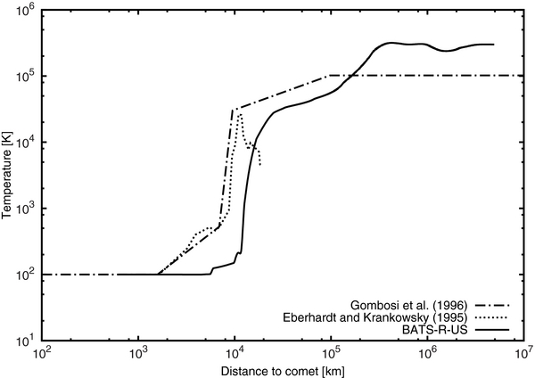
Figure 2. Electron temperature (K) along Giotto's inbound path. The x-axis denotes the distance from the comet (km). The solid line shows the modeled electron temperature compared to the model applied in Gombosi et al. (1996) which was derived from Häberli et al. (1995) and Eberhardt & Krankowsky (1995).
Download figure:
Standard image High-resolution imageFigure 3 shows the magnitude of the magnetic field during the inbound and then the outbound leg of Giotto together with the MAG measurements for comparison (Neubauer 1987). The sharp decrease in magnetic field strength inside the magnetic cavity is reproduced and marks the location where the magnetized plasma has no access, and therefore the innermost coma remains field-free. In some regions, our model does underestimate the magnetic field strength. While using a standard Parker spiral for the upstream magnetic field direction improves the result somewhat, but not altogether, the match to the plasma velocities, which will be discussed below, becomes worse. There are several other possible explanations for this discrepancy including the time-dependent variation of the solar wind conditions omitted in our steady-state simulation or gyro effects that cannot be fully self-consistently modeled with a fluid-type approach.
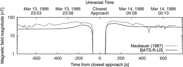
Figure 3. Magnetic field (nT) along the Giotto trajectory including inbound and outbound path. The x-axis indicates the time (s) from the closest approach on 1986 March 14, 00:03. Negative time indicates time before the closest approach (CA) and vice versa. The solid line shows the modeled magnetic field and the dashed line is taken from the Giotto magnetometer measurements (Neubauer 1987).
Download figure:
Standard image High-resolution imageFigure 4 shows the simulated ion bulk velocities compared to the measurements (Formisano et al. 1990; Altwegg et al. 1993). While the solar wind protons are deflected, the newly implanted light ions of cometary origin follow a pick-up distribution, which cannot accurately be reproduced by a fluid-type model. These effects combined with the energy range and acceptance angle of the JPA instrument (FIS: 0.01–20 keV e−1 and IIS: 0.09–90 keV e−1) that cuts out at least parts of the distribution, make a one-to-one comparison somewhat difficult. Close to the comet, i.e., inside ∼10,000 km from the nucleus, the velocity vectors and bulk speeds of the cometary ions are tightly coupled through ion–ion, ion–neutral, and ion–electron interactions while the solar wind protons are already attenuated in this region.

Figure 4. Ion velocities (km s−1) along Giotto's inbound trajectory. The x-axis denotes the distance to the comet (km) with the closest approach at roughly 600 km. The lines show the modeled bulk speeds of the solar wind protons, the cometary light ions, and the cometary heavy ions. The corresponding measurements are added, i.e., the heavy ion velocity by the JPA (Formisano et al. 1990) and the IMS (Altwegg et al. 1993) instruments, respectively.
Download figure:
Standard image High-resolution imageIn Figure 5, we show the simulated temperatures of the individual ion species from our model and compare them to those derived from the JPA instrument. For similar reasons as with Figure 4, we see a slight discrepancy between the modeled and measured heavy ion temperature because at least part of the energy distribution is not accessible to the JPA instrument. For the same reason, we might also underestimate the temperature of the cometary light ions in some regions. However, probably more important is that a fluid-type model is not perfectly suited to accurately represent the details of a pick-up ion population with the associated temperature.

Figure 5. Ion temperatures (K) along Giotto's inbound path. The x-axis denotes the distance to the comet (km). The lines show the modeled temperatures of the solar wind protons, the cometary light ions, and the cometary heavy ions. The corresponding measurements are also given: the observations of the protons and the heavy ions by the JPA (Formisano et al. 1990) and the IMS (Altwegg et al. 1993) instruments, respectively.
Download figure:
Standard image High-resolution image6.2. Detailed Plasma Distribution and Boundaries
Figure 6 shows the plasma mass densities (in amu cm−3) of the three modeled ion fluids, i.e., the solar wind protons in the top two plates, the cometary light ions in the middle two plates, and the cometary heavy ions in the lower two plates. The three plates on the left-hand side give a more global picture of the interaction of the comet with the solar wind, and the plates on the right focus on the region around the magnetic cavity. The x–y plane shown here is the plane containing the magnetic field. The solar wind is gradually slowed down and transitions to subsonic speeds at the bow shock, which is clearly visible in the top left plate. Its subsolar distance is roughly 400,000 km from the comet. Below, on the left-hand side, is the distribution of the cometary light ions that have a somewhat broader distribution than the cometary heavies (bottom plate) given the extended neutral atomic and molecular hydrogen distribution. There are also some clear asymmetries in the distribution of the involved species that we will discuss below.

Figure 6. Cuts with ion mass densities (amu cm−3) for the three ion groups, solar wind on top, the cometary light ions in the middle, and the cometary heavy ions at the bottom. The left panels show an overview with distances given in units of 106 km and the three plates on the right are close-ups around the magnetic cavity, contact surface, and ion pile-up with distances given in 104 km.
Download figure:
Standard image High-resolution imageThe top right panel in Figure 6 shows that the protons originating from the Sun vanish in the innermost region (∼10,000 km) due to the deflection around the cavity and the charge exchange as discussed in the previous section and shown by, e.g., Benna & Mahaffy (2007). Although the UV flux becomes attenuated in the innermost coma, there is a slight enhancement in particle density in the wake of the diamagnetic cavity. This is due to a small flow of plasma from behind toward the comet, an effect that we see for all the three fluids. The presence of the inner shock at the magnetic cavity boundary can be seen in both pick-up ion populations: the light and the heavy cometary ions (middle and lower right plates). Our results also indicate that both shocks are colocated where the magnetic pressure gradient force and the magnetic curvature force compensate the ion–neutral drag force (Cravens 1987). Therefore the species dependent drag coefficients in Equations (25) and (26) do not result in distinct shock positions for the different ion species, unlike the ion pile-up locations, which do not necessarily have to be colocated given the individual species' ion–electron recombination rates and the distribution of the corresponding neutrals. Also visible is the lack of ionization along the narrow region along the Sun–comet line in the wake of the comet. This is caused by the extinction of the solar UV photons responsible for the photoionization (Equations (19)–(21)).
The interaction of the ion fluids with each other through the Lorentz force is obvious: it can be seen in Figure 7 that the solar wind ions are deflected in the opposite direction from the cometary pick-up ions. The difference in their velocity with respect to the charge-averaged ion velocity from Equation (1) results in opposite signs in the Lorentz force term in Equations (4)–(6), and the gyration starts in the opposite direction. Together with a nonvanishing Bx component, the fluids are also getting deflected at an angle. One has to keep in mind that the MHD approach is not suitable to resolve the gyration of the individual ions as done in Hybrid-type models (e.g., Motschmann & Kührt 2006 or Delamere 2006); however, the general bulk motion of the fluids moving at different speeds can be reproduced by a multi-ion fluid model. This is also responsible for the asymmetric enhancement of the solar wind proton density discussed in Figure 1. From a numerical standpoint, it is quite expensive to reach a steady state solution due to oscillating fluids as they interact through the fields (Lorentz force) with each other, in particular in places where the frictional interaction between the fluids is small. As long as the solar wind is the dominant fluid, its flow direction remains almost unchanged (upstream of the bow shock as shown in Figure 7). As the mass density of the cometary pick-up ions starts to increase the back-coupling and the associated opposite deflection becomes obvious. When interpreting the plotted flow lines of the pick-up ion fluids, it should be noted that for stable numerical convergence the code by design requires positive, nonzero, mass densities for all the involved fluids in every computational cell. This requires the injection of heavy ions at the upstream boundary, although at a level several orders of magnitude lower than for the solar wind ions; we decided to inject them at the solar wind velocity. However, only after the fluid is dominated by the implanted, slow, pick-up ions does the deflection become apparent, i.e., at a few million kilometers from the nucleus.
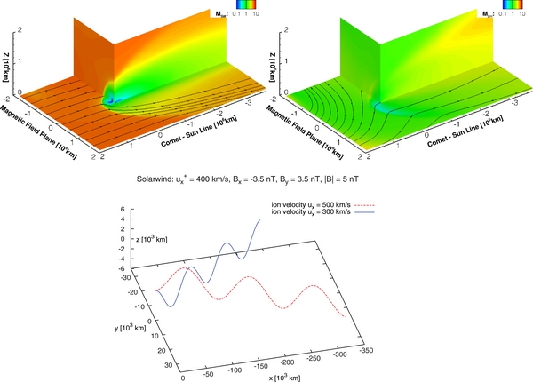
Figure 7. Top plots show the sonic Mach number and velocity streamlines, projected onto the plane of the undisturbed upstream magnetic field, for the solar wind (left) and the cometary heavy ions (right) from our model, respectively. For comparison, the bottom panel shows the gyration of two individual ions with initial velocity in the x direction of 300 km s−1 and 500 km s−1, respectively, when the charge averaged bulk ion velocity is 400 km s−1 and the magnetic field is at an angle of 45° (non-vanishing Bx component) in the x–y plane with a magnitude of 5 nT (note the different axis scales). While the gyration of the individual ions cannot be reproduced in multifluid MHD, the general interacion of the bulk of the fluids with the magnetic field through the Lorentz force can (see Equations (4)–(6)).
Download figure:
Standard image High-resolution imageThen, closer in, as the plasma slows down and the interaction with the neutral background atmosphere becomes more dominant (the three plates on the right hand side of Figure 6), the effect of the Lorentz force becomes less important. The flow lines inside and close to the magnetic cavity boundary are quite similar for both pick-up ion populations.
As discussed in the previous section, Giotto observed a rapid decrease in magnetic field strength around the closest approach. Figure 8 shows the magnitude of the magnetic field and the associated magnetic field lines. The magnetic field is piled-up in front of the magnetic cavity and draped around it. As mentioned above the magnetic pressure gradient and curvature forces balance the ion–neutral charge exchange at the location of the shock, and inside the cavity the plasma is supersonic and entrained in the outflowing neutral gas. Consequently, the magnetized plasma originating from further upstream on the sunward side does not penetrate the cavity, and the magnetic field is absent in this innermost region (with the assumption in our model that the comet does not carry any residual magnetization).

Figure 8. Magnetic field magnitude (nT) and magnetic field lines projected onto the plane of the undisturbed magnetic field. The left panel shows an overview with distances given in units of 106 km and the plate on the right is a close-up showing the draping of the field around the magnetic cavity with distances given in 104 km.
Download figure:
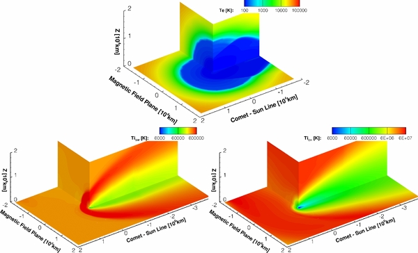
Standard image High-resolution imageFigure 9 shows the electron temperature in the vicinity of the comet. The innermost region is efficiently cooled by inelastic collisions with the abundant neutral water molecules (Gan & Cravens 1990). Then, at roughly 10,000 km, the electron temperature increases sharply and can be associated with the formation of the ion pile-up by suppression of the ion–electron recombination. The same figure also shows an overview of the modeled temperatures of the solar wind and the cometary heavy ions. Far upstream of the bow shock where cometary heavy ions are implanted at almost zero velocity into the already accelerated heavy ion plasma, the temperature is much higher than for the solar wind. The solar wind protons reach their maximum temperature at the location of the bow shock where the plasma is decelerated and compressed as it transitions from supersonic to subsonic speeds. Close in, the plasma is slowed down and cooled by collisions with the neutral gas. Furthermore, the plasma of cometary origin is also dominated by ions picked-up at low velocity, which in combination with the collisions with the neutrals further decreases the plasma temperature. Since there is no source of mass loading for the solar wind ions, their only way to shed thermal energy are elastic collisions.
Figure 9. Top plate shows the modeled electron temperature (K) in the close vicinity of the diamagnetic cavity and contact surface. The sharp temperature increase outside this area is partially responsible for the formation of the ion pile-up (distances in units of 104 km). The bottom panel shows an overview of the modeled ion temperatures (K) of the solar wind (left) and the cometary heavy ions (right), respectively (distances given in units of 106 km). The cometary heavy ions are much hotter due to the pick-up process compared to the solar wind protons which reach their maximum temperature at the bow shock where they are compressed as the flow is decelerated from supersonic to subsonic speeds.
Download figure:
Standard image High-resolution image
7. SUMMARY AND CONCLUSIONS
In this article, we compare the results of our multifluid MHD model to the observations obtained by the instruments on board Giotto during the fly-by at comet 1P/Halley on 1986 March 14. The validated model can then be used to study the global scale interaction of the comet with the solar wind and to put the obtained measurements in their context.
Our results suggest that the plasma bulk speeds and temperatures of the individual ion species stay coupled inside the ion pile-up region (∼20,000 km). Then, farther away from the comet, the individual plasma populations, given their distinct velocities, clearly interact with each other through the Lorentz force. Fast solar wind protons and the implanted slower cometary ions are deflected in opposite directions.
The temperature of the pick-up ions reaches up to 108 K and is thus much hotter than the solar wind temperature (∼300,000 K), a finding that is in accordance with the observations. The model is capable of qualitatively reproducing the sharp increase of the electron temperature in the ion pile-up region that is responsible for the reduction in the ion–electron recombination rate. Inside the cavity, the electrons are efficiently cooled by inelastic electron-H2O collisions. The model is also able to reproduce the basic plasma boundaries including the magnetic cavity (∼4500 km in the sunward direction) and the associated inner shock, as well as the bow shock (∼400,000 km upstream). The inner shock is colocated for the different plasma species, while the ion pile-up location and shape can show slight differences between the different species. Solar wind protons vanish in the vicinity of the comet, i.e., inside the ion pile-up region.
Of course, while getting a satisfactory match to the observations, the results have to be understood within the limitations of the chosen fluid approach. Nevertheless, they are very encouraging for a future comparison with hybrid-type models that capture the finite gyro radii of the ions (see Hansen et al. 2007) and to see whether some of the resulting plasma features can be reproduced by multifluid MHD.
This work has been supported by the Swiss National Science Foundation, the US Rosetta Project by JPL subcontract 1266313 under NASA grant NMO710889, NASA Planetary Atmospheres program grant NNX09AB59G, grant AST-0707283 from the NSF Planetary Astronomy program, and by a grant from the Swiss National Supercomputing Centre (CSCS) under project ID s402. We would also like to acknowledge the help and support of the comet modeling groups sponsored and partially funded by the International Space Science Institute (ISSI), Bern, Switzerland. Finally, we thank the reviewer for assistance in evaluating this article.