


ABSTRACT
We report white-light observations of a fast magnetosonic wave associated with a coronal mass ejection observed by STEREO/SECCHI/COR1 inner coronagraphs on 2011 August 4. The wave front is observed in the form of density compression passing through various coronal regions such as quiet/active corona, coronal holes, and streamers. Together with measured electron densities determined with STEREO COR1 and Extreme UltraViolet Imager (EUVI) data, we use our kinematic measurements of the wave front to calculate coronal magnetic fields and find that the measured speeds are consistent with characteristic fast magnetosonic speeds in the corona. In addition, the wave front turns out to be the upper coronal counterpart of the EIT wave observed by STEREO EUVI traveling against the solar coronal disk; moreover, stationary fronts of the EIT wave are found to be located at the footpoints of deflected streamers and boundaries of coronal holes, after the wave front in the upper solar corona passes through open magnetic field lines in the streamers. Our findings suggest that the observed EIT wave should be in fact a fast magnetosonic shock/wave traveling in the inhomogeneous solar corona, as part of the fast magnetosonic wave propagating in the extended solar corona.
Export citation and abstract BibTeX RIS
1. INTRODUCTION
Associated with coronal mass ejections (CMEs) and flares are fast magnetosonic waves that are triggered to propagate in all directions into the corona with a local characteristic fast magnetosonic speed. They can be driven to form a shock (e.g., Sheeley et al. 2000) that propagates radially in the extended corona with a speed range of 765–930 km s−1 (Robinson 1985). These MHD shocks can cause plasma oscillations owing to charge separation at the shock front accelerating electron that produce radio emission, called type II radio bursts (Uchida 1960; Wagner & MacQueen 1983). Because of the faster characteristic speed in the higher corona (Gopalswamy et al. 2001), the propagating fast magnetosonic wave in the extended solar corona tends to be refracted toward the solar surface and impacts the chromosphere (Uchida 1968; Afanasyev & Uralov 2011). It is thought that the impacted wave energy on the chromosphere can produce strong down-up flows that can be observed as a propagating disturbance in Hα wings against the chromospheric disk. The disturbance is known as the Moreton wave, with speeds of ∼1000 km s−1 (Moreton 1960; Uchida 1968; Asai et al. 2012).
These types of disturbances have also been termed "EIT," "EUV," or "coronal" waves (hereafter EUV disturbances) in the literature (Warmuth & Mann 2011, and references therein) because they are observed by imaging telescopes in the extreme-ultraviolet (EUV) passbands, as large-scale disturbances globally traveling across the solar disk with a shape that is partially circular with typical speeds of 100–500 km s−1 (Moses et al. 1997; Thompson et al. 1999, 2009). They occasionally show the characteristics of waves, such as reflection and refraction of fronts at the boundaries of coronal holes and active regions (Wills-Davey & Thompson 1999; Veronig et al. 2006; Gopalswamy et al. 2009; Li et al. 2012; Liu et al. 2012; Olmedo et al. 2012). Furthermore, they have also been reported to stop or decelerate at boundaries of coronal holes and active regions and remain in the form of stationary fronts at these boundaries for a few minutes to a few hours (Thompson et al. 1999; Delannée & Aulanier 1999; Delannée 2000; Attrill et al. 2007; Delannée et al. 2007). Because of the direction of their propagation and the morphology, EUV disturbances had been thought to be fast magnetosonic waves. Numerical simulations have been able to reproduce their typical characteristics, including wave reflection and refraction in support of their fast magnetosonic wave interpretations (Wang 2000; Wu et al. 2001; Ofman & Thompson 2002; Schmidt & Ofman 2010; Downs et al. 2011, 2012).
Interestingly, the characteristics of EUV disturbances can also be explained by non-wave or pseudo-wave scenarios, namely, the magnetic reconfiguration scenario (Delannée & Aulanier 1999; Chen et al. 2002; Chen 2009; Warmuth & Mann 2011). The basic idea is that there exist globally connected closed magnetic field lines overlying an active region where a CME occurs. According to this scenario, the outgoing CME pushes up the overlying closed magnetic field lines from the inside to the outside, causing the legs of the closed magnetic field lines to stretch. As a result, bright fronts can appear propagating away from the erupting site, like what is seen in the observations of EUV disturbances. These bright fronts could be a consequence of plasma compression and/or heating at the legs of the stretched magnetic field lines (Attrill et al. 2007; Chen et al. 2002; Chen 2009; Delannée & Aulanier 1999; Delannée 2000; Delannée et al. 2007, 2008). Accordingly, the propagating fronts must stop at the end of the closed magnetic field lines, or separatrices; therefore, these scenarios can explain why EUV disturbances appear to stop at the boundaries of coronal holes and active regions in the form of stationary fronts. Moreover, the slow speeds of EUV disturbances can be easily understood since the propagating fronts are a result of the restructuring of the global magnetic field framework (Chen et al. 2002), rather than true propagating waves.
What are the expected observational manifestations of the fast magnetosonic waves in the solar corona, as distinguished from the ones of the magnetic reconfiguration scenario? If a disturbance occurs, then part of the energy of that disturbance can be transferred efficiently in the direction normal to the magnetic field lines and can effectively compress magnetic fields and plasma at the front of the disturbance. These waves, as seen from a "top" view, may be observed as a circularly propagating disturbance against the solar disk due to radial magnetic field lines aligned toward the observer, like EUV disturbances. From a "side" view, as the waves propagate perpendicular to the magnetic field lines in the extended corona, the disturbances may be seen as a density compression along the field lines. Note that these radial and moving density compressions can also be explained by the magnetic reconfiguration scenario as described above. However, according to the scenario, such disturbances must stop at the end of the closed magnetic field lines (e.g., Chen et al. 2002), for example, at the boundary of coronal streamers (cf. Figure 22 in Schrijver et al. 2011), where the global magnetic field connectivity changes (magnetic separatrix; Sturrock & Smith 1968), while fast magnetosonic waves can freely pass through at the local fast magnetosonic speed.
The COR1 inner coronagraphs (Thompson et al. 2003) on board the Solar TErrestrial RElations Observatory (STEREO; Kaiser et al. 2008) spacecraft are the most appropriate for the observation of density compressions along radial magnetic field lines in the extended corona ranging from 1.5 to 4 R☉. COR1 images represent the amount of scattered polarized light due to electrons in the corona, so that the intensity at each pixel is proportional to the electron density along the corresponding line-of-sight direction. If a front of compressible MHD waves lies on the plane of the sky, the wave front can be observed as an intensity enhancement. STEREO consists of twin spacecraft, Ahead and Behind, that move nearly along Earth's orbit around the Sun in opposite directions relative to the Earth, so that the twin spacecraft provide observations at two different viewpoints simultaneously and independently. The simultaneous and independent observations allow us to observe the wave fronts, which are generally faint and therefore noisy, from multiple vantage points.
In this paper we report novel observations of a fast magnetosonic wave propagating across solar radial background magnetic fields, passing through streamers, with local fast magnetosonic speeds in the extended corona observed by COR1 inner coronagraphs. These observations help clarify the wave nature of EUV disturbances typically observed on the solar disk. In Section 2, we describe the data that afford us the opportunity to investigate the "top" and "side" views of propagating disturbances. In Section 3, we show detailed properties of propagating disturbances and their physical implications. A summary and conclusion are given in Section 4.
2. DATA
Here we study the coronal disturbance associated with a flare and CME event of 2011 August 4 at 03:50 UT. For this investigation, we use white-light images obtained by the COR1 inner coronagraphs (Thompson et al. 2003) and full-disk EUV images at the 195 Å passband taken by the Extreme UltraViolet Imager (EUVI; Wülser et al. 2004) on board the STEREO spacecraft. At that time, the separation angle between STEREO Ahead and Behind was ∼167°, and the two spacecraft were able to observe the extended solar corona from nearly opposite directions. COR1 images consist of 512 by 512 pixels with a resolution of 15 arcsec pixel−1 and a corresponding projected physical scale for 2 pixels of 21 and 23 Mm on Ahead and Behind images, respectively. The EUVI instrument provides images of 2048 by 2048 pixels with resolution 1.6 arcsec pixel−1 and a projected physical scale for 2 pixels of 2.2 Mm. The time cadence of COR1 total brightness images and EUVI 195 Å images is 5 minutes. The basic calibrations of all data are carried out with "secchi_prep.pro" of the SolarSoftware library.
3. RESULT AND DISCUSSION
3.1. Trajectory of Coronal Disturbance
Figure 1 shows time-series observations of the solar corona observed by COR1 Behind (Figures 1(a)–(d)), COR1 Ahead (Figures 1(e)–(h)), and EUVI 195 Å Ahead (Figures 1(i)–(l)). Figures 1(a) and (e) show total brightness images combined with three polarized images (0°, 120°, and 240°; Thompson et al. 2003), and the rest are running difference images that are subtracted by prior time-step images to enhance the changes during the time intervals (5 minutes). In order to show the changes, we applied byte scaling to the running difference images of COR1 and EUVI with values in the range of [−2.3, 1.7] × 10−9 and [−10, 10], respectively. These images show propagating disturbance seen as a radial density compression propagating azimuthally by COR1 inner coronagraphs and as a circularly radially propagating EUV disturbance by EUVI (see also Movies 1 and 2). When the flare occurred, an expanding and outgoing spherical pulse (Veronig et al. 2010; Li et al. 2012) was observed by EUVI at 03:55 UT (Figure 1(i)). After that, a vertical and thin coronal disturbance (hereafter COR1 disturbance) was observed beside the expanding lateral flank of the spherical wave pulse (arrows in Figures 1(b)–(d) and 1(f)–(h); see also Patsourakos & Vourlidas 2009; Patsourakos et al. 2010; Cheng et al. 2012). The COR1 disturbance passed through various coronal regions, such as the active/quiet corona, coronal holes, and streamers. In the field of view (FOV) of EUVI Ahead the EUV disturbance was observed as a bright front (arrows in Figures 1(j)–(l)) that propagates away from the flare site with a partially circular shape.
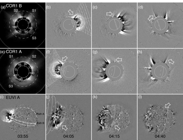
Figure 1. Event observed on 2011 August 4 at 03:55 to 04:40 UT with STEREO Ahead and Behind. Images show STEREO COR1 Behind ((a)–(d)), Ahead ((e)–(h)), and EUVI 195 Å Ahead ((i)–(l)) observations. Panels (a) and (e) show total brightness images of COR1, and circles inside occulting disks demarcate the disk of the Sun, labeled with position angle (P.A.), with zero at the approximate flare site projected on the image planes. Panels (b)–(d), (f)–(h), and (i)–(l) show running difference images. In panels (b), (f), and (j), solid lines passing through the solar center and flare site (cross symbol in (j)) are set to the axis of a cone representing the three-dimensional structure of the COR1 disturbance. Concentric circles show the surface of the modeled cone at heliocentric distances from 1 to 5.5 R☉ in intervals of 0.5 R☉. In the remaining images, taken after 04:05 UT, only the intersection of the cone with the solar surface is represented with solid and dashed curves for the front and backside of image planes, respectively. In panel (i), dashed curves represent Paths A and B to construct time–distance maps in panels (c) and (d) in Figure 2. The region enclosed by two solid curves is used to measure the speed of the EUV disturbance. Arrows refer to the representative fronts of COR1 and EUV disturbances. These STEREO Ahead and Behind observations are also available as mpeg Movies 1 and 2 in the online version of the Astrophysical Journal, respectively: left panels of the movies show composite images of COR1 total brightness images and EUVI running difference images. Red boxes in the movies represent the FOV of the EUVI observations. Right shows COR1 and EUVI running difference images. Plus symbols in the movies refer to the fronts of the propagating fast magnetosonic wave at 1.6, 2.0, 2.5, and 3.0 R☉, respectively.(Animations (1a and 1b) of this figure are available in the online journal.)
Download figure:
Standard image High-resolution imageIn order to find the spatial and temporal relationship between the COR1 and EUV disturbances, we have modeled the three-dimensional structure of the COR1 disturbance using a triangulation method (Kwon et al. 2010) assuming that the COR1 disturbance expanded from the flare site with the shape of a cone (Appendix A; cf. Xie et al. 2004; Patsourakos et al. 2009). Figures 1(b), (f), and (j) show the modeled cone with concentric circles from the solar surface to 5.5 R☉ in intervals of 0.5 R☉. In the rest of the images taken after 04:05 UT, only the cone's surface at the heliocentric distance of 1 R☉ is plotted to show the footpoint of the COR1 disturbance. The footpoint is spatially in good agreement with the front of the EUV disturbance as seen in the EUVI images. From this three-dimensional analysis, we found that the COR1 disturbance is propagating above the EUV disturbance, implying that the origin of the COR1 and EUV disturbances may be the same (Grechnev et al. 2011a).
Time–distance plots showing the wake of the coronal disturbance are given in Figure 2. These plots are made by stacking strips cut along a path on a sequence of images over a specified time range; thus, we construct a stack plot where the abscissa is the distance and time is the ordinate. In this plot, any motion along the path may appear as an oblique line. Figures 2(a) and (b) show the wakes of the COR1 disturbance observed by COR1 Ahead and Behind, along paths taken at a heliocentric distance of 2.5 R☉, as denoted by dashed circles in Figures 1(e) and (a), respectively. These two plots clearly show that the COR1 disturbance propagates in either direction away from the origin, which is located at the flare site. The COR1 disturbance reached a position angle (P.A.) of ∼130° to the north and a P.A. of ∼−80° to the south before becoming too faint to track. When the disturbance reached a P.A. of ∼130°, it appears to pass through a region where another CME occurred, though whether or not that CME was triggered by the disturbance is not clear. The wake of the COR1 disturbance also passes through coronal streamers 1, 2, and 3 denoted by S1, S2, and S3 in Figures 1(a) and (e) located at a P.A. of ∼40° (S1), 100° (S2), and −60° (S3), respectively. As a result of the passage of the COR1 disturbance through these streamers, the streamers were deflected and then bounced back to their initial positions. Note that the deflections are observed not only on streamers 1 and 3 near the CME site but also on streamer 2 in the distance, indicating that the disturbance was transferred to a distant site, regardless of the likely existence of separatrices along its path. Streamer deflections far away from flare/CME sites have been well reported by many authors (Sheeley et al. 2000; Filippov & Srivastava 2010; Feng et al. 2011). This is significant because it indicates that the nature of the disturbance is that of a fast magnetosonic wave instead of large-scale magnetic restructuring as suggested by the magnetic reconfiguration scenario.

Figure 2. Time–distance maps constructed by running difference images. Panels (a) and (b) show the trajectories of the COR1 disturbance along paths taken at a heliocentric distance of 2.5 R☉ represented by dashed circles in Figures 1(e) (COR1 Ahead) and 1(a) (Behind), respectively. The abscissa represent P.A. centered at flare site, and the ordinate is accumulated time in hours from 03:55 UT. In panel (a), vertical dashed lines represent the locations of streamers. Cross symbols denote the determined positions of the propagating COR1 disturbance. Panels (c) and (d) show the wakes of the EUV disturbance along Paths A and B denoted by dashed lines in Figure 1(i). Arrows in panel (c) point to the locations of stationary fronts (SF1a, SF1b, and SF2). Plus symbols in panel (d) refer to the fronts of the EUV disturbance, and the dashed line is the result of a first-order least-squares polynomial fit.
Download figure:
Standard image High-resolution imageThe trajectories of the EUV disturbance show that what appear as fronts on the inhomogeneous solar surface (low solar corona) can be attributed to the passage of the COR1 disturbance. Two great circle paths lying along the surface are considered and compared. Path A in Figure 1(i) passes through the quiet corona and coronal holes, and Path B lies only in the quiet corona. Stack plots made along Paths A and B are shown in Figures 2(c) and (d), respectively. While the bright front of the EUV disturbance is seen to propagate uninterrupted along Path B, the trajectory along Path A shows discrete and long-lasting brightenings (three arrows, S1a, S1b, and S3), known as stationary fronts (Attrill et al. 2007; Delannée & Aulanier 1999; Delannée 2000; Delannée et al. 2007). Furthermore, it is seen that the EUV disturbance did not stop at the sites of the stationary fronts but crossed them and passed to the quiet corona to reach a distant site where the wave energy seems to be transferred to stationary front 3 pointed at by the third arrow at P.A. of ∼90° in Figure 2(c).
Path A lies nearly along the plane of the sky to the north; therefore, the trajectory can be directly compared with what is observed in COR1. Figure 3 provides us with a combined image of COR1 and EUVI Ahead taken at 05:00 UT, near P.A. ∼45°, and shows that Path A passes through stationary fronts 1a and 1b in the EUVI image below streamer 1 in the COR1 image. The two stationary fronts were located at the boundaries of coronal holes that are connected by closed loops seen as dark threads below the streamer. Note that coronal streamers are a mixture of closed magnetic fields close to the solar surface that become open in the higher corona (Sturrock & Smith 1968). This figure demonstrates that stationary fronts 1a and 1b were located at the footpoints of streamer 1. In this context, the EUV disturbance may be interrupted by the closed magnetic field structure, while COR1 disturbance freely penetrates the streamer through the open magnetic fields above closed magnetic fields. The COR1 disturbance reached the remote site where a third stationary front (S2) was located. The absence of a continuous trajectory between stationary fronts 1b and 2 seen in Figure 2(c) provides evidence for a wave front traveling above the closed magnetic fields in the extended corona.
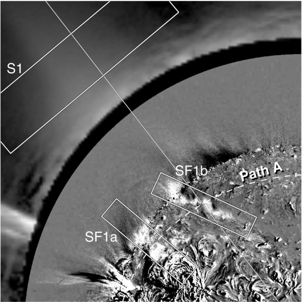
Figure 3. Composite image of EUVI and COR1 Ahead taken at 05:00 UT. The EUVI image is running difference, and the COR1 image is total brightness. Two boxes in the EUVI image highlight the stationary fronts 1a and 1b corresponding to the first two arrows in Figure 2(c). Another box in the COR1 image is located at a heliocentric distance of 1.9 R☉ across the axis of streamer 1. The boxes are used to construct time-series images in Figure 4. Dashed curve refers to Path A. Solid line represents the direction from the solar disk center to stationary front 1b to show spatial correlation of the stationary fronts with streamer 1.(An animation of this figure is available in the online journal.)
Download figure:
Standard image High-resolution image3.2. Stationary Front and Streamer Oscillation
Because stationary fronts 1a and 1b lie close to the solar limb (Figure 3), their temporal evolution can be compared with what is observed by the COR1 A coronagraph directly. Figure 4 shows time series of total brightness images of streamer 1 at a heliocentric distance of 1.9 R☉ (top) and running difference images of stationary fronts 1a (middle) and 1b (bottom), taken from the boxes shown in Figure 3 at time steps from 03:30 UT to 06:30 UT in intervals of 10 minutes. The arrows on the left side on the panels indicate the direction of the initial disturbance. According to the top panel, the COR1 disturbance first appeared as a density enhancement inside the streamer at 04:00 UT and at that time the streamer started to deflect in the direction of the initial disturbance. At 04:20 UT, the displacement of the axis of the streamer reached the maximum and started to bounce back to its initial position. As for the EUV disturbance shown in the middle and bottom panels, they were first observed at 04:00 UT simultaneously as the COR1 disturbance swept above these regions and started to dim at 04:10 UT. After the streamer started to bounce back toward its initial position, stationary front 1b began to emerge at 04:30 UT, and approximately 20 minutes later stationary front 1a emerged at 04:50 UT. An arrow in the middle of this figure points to the stationary fronts when they first showed up. The two stationary fronts lasted until approximately 06:30 UT.
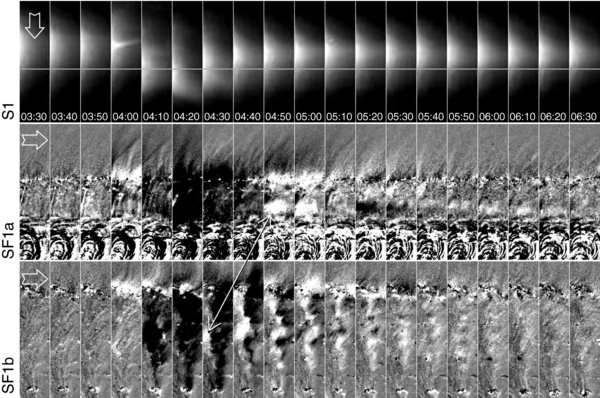
Figure 4. Temporal evolutions of streamer 1 and stationary fronts 1a and 1b. Top panel shows time-series images in an FOV highlighted by a box across the axis of streamer 1 at a heliocentric distance of 1.9 R☉ (Figure 3). Solid horizontal line in the top is the same as in Figure 3. Middle and bottom panels show the co-temporal time series of stationary fronts in fields of view demarcated by rectangles in Figure 3. The direction of the coronal disturbance is indicated by an outlined arrow in each panel. An arrow in the middle of this figure points to the stationary fronts 1a and 1b when they first came into sight. Time of these time-series images is shown at bottom in the top panel in UT.
Download figure:
Standard image High-resolution imageIt is significant to note that the stationary fronts appear as a pair at the footpoints of the streamer and the order of the appearances of two stationary fronts is in the opposite direction of the coronal disturbance or the expanding lateral flank of the CME. Note that the order is consistent with the direction of the streamer's bouncing-back motion and its timing. If the stationary fronts 1a and 1b were directly formed by stretched magnetic field lines due to outgoing CME, the front must stop at the end (footpoint) of the magnetic field lines overlying the outgoing CME, that is, the site of stationary front 1a. Moreover, no matter what the stationary front can be transferred from the site of 1a to another footpoint of the streamer owing to the expanding CME bubble; the stationary fronts should be formed in the same order as the magnetic field lines are restructured, from inside to outside. As clearly shown in Figure 4, however, the stationary front 1b appears before 1a, along the same lines of the direction of the streamer's bouncing-back motion (see also Movie 3). These observational facts suggest that the stationary fronts should be understood by the streamer's bouncing-back motion, rather than the reconfiguration of magnetic field lines overlying the outgoing CME.
A subsequent question that is naturally raised here is whether the swing motion of the streamer is in fact a kink mode wave or not. Deflections of coronal streamers have been reported to be associated with flares/CMEs, but their physical nature is still unclear (Sheeley et al. 2000; Chen et al. 2010; Filippov & Srivastava 2010; Feng et al. 2011). In order to study the nature of the streamer's swing motion, we applied a model fitting to the motion of streamer 1 that showed the clearest stationary fronts at its footpoints. We used the damped sine function written as follows:
where the parameters A0, τ, and P refer to initial amplitude, e-folding damping time, and period, respectively (e.g., Nakariakov et al. 1999; Ofman & Aschwanden 2002; White & Verwichte 2012; Liu et al. 2012). We used this function to determine the period P and damping time τ of the streamer's motion at several heliocentric distances. To fit the displacement of the axis of the streamer at each heliocentric distance, we constructed time–distance maps across the axis of the streamer. The top panel in Figure 5 is the time–distance map showing the swing motion of the streamer taken at heliocentric distances of 2.0 (left), 2.5 (middle), and 3.3 R☉ (right). The signal along a slice at a time step is defined as a value that is 1.5 times the standard deviation plus the average of the intensity over the slice. Each location is weighted by the corresponding intensity. To perform the fitting, we used "mpfitfun.pro" in IDL library. Dashed-dot, dashed, and solid curves in the top panel represent the axis of the streamer varying with time, determined by the fitting. The bottom panel provides us with a comparison of the three results of the model fitting at these heliocentric distances and shows that the swing motion propagates upward as its period increases with the heliocentric distance.

Figure 5. Oscillatory motion of streamer 1. Top panel shows time–distance maps across the axis of streamer 1 at heliocentric distances of 2.0 (left), 2.5 (middle), and 3.0 R☉ (right). The abscissa is distance from the initial position of the axis, and ordinate is accumulated time from 04:05 UT. Dashed-dot, dashed, and solid curves represent the oscillating axis at these heliocentric distances found by least-squares fitting with Equation (1). These curves are plotted together in the bottom panel.
Download figure:
Standard image High-resolution imageAccording to analytical results and observations (e.g., Hollweg & Yang 1988; Ofman & Aschwanden 2002; Ruderman & Roberts 2002; White & Verwichte 2012), the damping time of a kink mode wave is nearly proportional to its period. Figure 6 shows the relationship between damping times and periods determined at heliocentric distances ranging from 2.0 to 3.3 R☉ in intervals of 0.1 R☉. The two quantities are strongly correlated with a coefficient of 0.87, suggestive of a quickly damped kink mode wave (cf. Ofman & Aschwanden 2002; Liu et al. 2012; White & Verwichte 2012). These facts demonstrate that part of the energy of the waves traveling in the extended corona may be trapped in streamers as kink mode waves (Aschwanden et al. 1999; Nakariakov et al. 1999; Sheeley et al. 2000; Chen et al. 2010; Liu et al. 2012). This energy absorption may cause stationary fronts with local density enhancements resulting from either density compressions due to trapped waves inside streamers, strong plasma up–down flows due to interactions between waves and magnetic structures of streamers, or a combination of these effects.

Figure 6. Damping times vs. periods of oscillatory motion on streamer 1, determined at heliocentric distances from 2.0 to 3.3 R☉ in intervals of 0.1 R☉. Dashed line is the result of a first-order least-squares polynomial fit, and the correlation coefficient is 0.87.
Download figure:
Standard image High-resolution image3.3. Speed of Coronal Disturbance
In order to confirm that the coronal disturbances observed by EUVI and COR1 are in fact fast magnetosonic waves, the speeds should be checked for whether they are consistent with properties of the coronal medium, such as magnetic field strength, electron density, and temperature. For instance, Zhao et al. (2011) measured speeds of EUV waves observed in 2010 January 17 and estimated local fast magnetosonic speeds using magnetic field strengths, electron densities, and plasma properties determined by models. They found positive correlations between the two speeds and conclude that EIT waves are in fact fast magnetosonic waves. In this paper, we estimate magnetic field strengths as a function of heliocentric distance using determined speeds and electron density. If the speeds of the observed coronal disturbance are in fact fast magnetosonic speeds in the solar corona, the estimated magnetic field strengths should be consistent with the coronal magnetic field strengths expected from theoretical and empirical models.
To achieve this goal, we measured the traveling distances of the COR1 disturbance by visual inspections along circular paths at heliocentric distances of 1.6, 2.0, 2.5, and 3.0 R☉ in COR1 Ahead and Behind images when the disturbance passes between two streamers (cross symbols in Figures 2(a) and (b); see also Movies 1 and 2). Since the visual inspection may cause errors due to biases in the measurement and image scaling/binning, we repeated the measurements nine times, changing the image scaling/binning each time. As for the front of the EUV disturbance, 14 paths were chosen along great circles on the solar surface in the quiet-Sun region enclosed within the two solid curves in Figure 1(i). The traveling distances of the EUV disturbance were determined by visual inspections along the paths. For instance, cross symbols in Figure 2(d) represent the measured position of the fronts along Path B. Figure 7 shows the average distances over the repeated measurements with circles and their standard deviations with error bars and suggests that the coronal disturbance traveling in the higher corona sweeps through a larger distance during the same time interval.
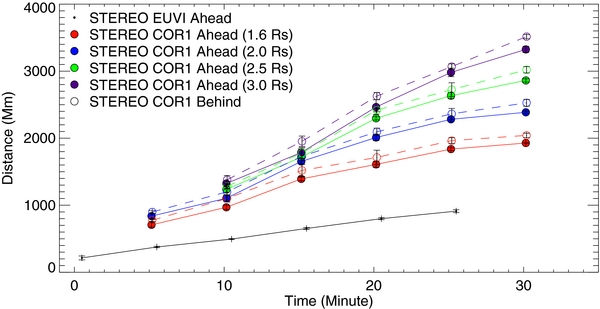
Figure 7. Traveling distances of EUV and COR1 disturbances. The traveling distances of the COR1 disturbance are measured along circular paths on image planes with heliocentric distances of 1.6, 2.0, 2.5, and 3.0 R☉. The traveling distances of the EUV disturbance are measured along great circle paths enclosed within the two solid curves in Figure 1(i). Each value and error bar represents average and standard deviation over repeated measurements. Closed circles (solid lines) and open circles (dashed lines) refer to the measured distances with STEREO Ahead and Behind, respectively.
Download figure:
Standard image High-resolution imageFigure 8 shows the determined speeds of the COR1 and EUV disturbances using the trajectory shown in Figure 7. Each closed circle refers to average speed traveling a section represented by an error bar of P.A. For instance, the first point in the panel of Ahead 2.5 R☉ refers to an average speed of the COR1 disturbance traveling between P.A. ∼40° and 60° at a heliocentric distance of 2.5 R☉. The error in speed is determined by uncertainty in traveling distance, as shown in Figure 7, and uncertainty in time. The uncertainty in time is caused by the fact that total brightness images are combined by three polarized images. The time cadence of the polarized images is 12 s, so we took 24 s as the uncertainty in time. The solid curve in each panel for the COR1 disturbance refers to the intensity normalized to an arbitrary value, along the corresponding path. All panels representing the speeds of the COR1 disturbance show a similar behavior of which the speeds are the highest when the disturbance travels in the coronal hole/quiet corona (low-intensity region) and decelerate as it approaches a dense region (streamer 2). For instance, the speeds at 2.5 R☉ (Ahead) were determined to be 1607 ± 193, 1933 ± 185, 1125 ± 179, and 757 ± 167 km s−1. In the case of the intensity at a heliocentric distance of 1.6 R☉ observed by Ahead, the circular path is close to the boundary of the occulting disk of COR1 images, so the intensity profile is very noisy. The tendency is consistent with what is expected, that the Alfvén speed should be faster in a region where electron density is lower. Meanwhile, the speeds of the EUV disturbance are 544 ± 97, 393 ± 33, 528 ± 48, 487 ± 48, and 373 ± 74 km s−1.
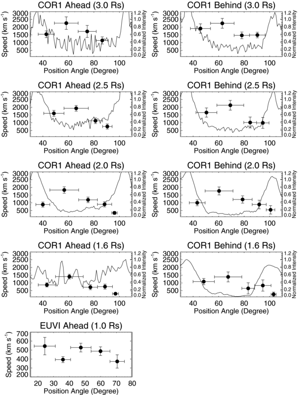
Figure 8. Speeds of COR1 and EUV disturbances. The speeds of the COR1 disturbance observed by Ahead (left) and Behind (right) are measured when the disturbance travels between streamers 1 and 2. Bottom panel shows the speeds of the EUV disturbance. Vertical error bars represent the errors in speeds due to uncertainties in traveling distance and time. Horizontal error bars denote the sections where the speeds are measured. Solid curves show intensity profiles normalized to arbitrary values along the corresponding circular paths.
Download figure:
Standard image High-resolution imageNext, we estimated magnetic field strengths as a function of heliocentric distance using measured speeds and electron densities and a constant temperature. The speeds of the coronal disturbances in Figure 8 show that the coronal medium is highly inhomogeneous, and the speeds may allow us to measure the inhomogeneous magnetic field strengths. In this paper we only consider the variations of physical quantities in the radial direction, not in the azimuthal direction since radial profiles of physical quantities are easily compared with empirical and theoretical models, and then check whether or not the observed coronal disturbance is in fact a fast magnetosonic wave.
To do this, we took averages and standard deviations of the speeds over the traveling region at 1.0, 1.6, 2.0, 2.5, and 3.0 R☉, and they are 465 ± 78, 829 ± 389, 1059 ± 469, 1402 ± 497, and 1723 ± 394 km s−1, respectively (closed circles and error bars in Figure 9(a)). Note that this is consistent with the tendency that the characteristic Alfvén speed increases with heliocentric distance until ∼4 R☉ (Gopalswamy et al. 2001). As for electron density, three-dimensional electron density in the heliocentric distance range of 1.2–4.0 R☉ was measured by a tomographic reconstruction method (Kramar et al. 2009) using EUVI and COR1 observations (see Appendix B). The averages and standard deviations of determined electron densities are (1.3 ± 0.1) × 108, (6.0 ± 0.5) × 106, (1.3 ± 1.1) × 106, (3.5 ± 3.4) × 105, and (1.6 ± 1.4) × 105 cm−3 at 1.0, 1.6, 2.0, 2.5, and 3.0 R☉, respectively. Figure 9(b) shows the average electron density as a function of heliocentric distance. Here we postulate that all wakes of the propagating disturbance are purely perpendicular to the magnetic field lines that are parallel to each other, and we neglect any possible effects of structures across the fields on the wave phase speeds. Closed circles and error bars in Figure 9(c) refer to the estimated magnetic field strengths using the average speeds and electron densities (see Appendix C). We found magnetic field strengths of 2.5 ± 0.5, 1.0 ± 0.5, 0.6 ± 0.4, 0.4 ± 0.2, and 0.3 ± 0.2 G at the heliocentric distances of 1.0, 1.6, 2.0, 2.5, and 3.0 R☉, respectively. As seen in Figure 9(b), our results are consistent with magnetic field strengths found empirically in the quiet corona (Mann et al. 1999; solid curve) and active corona (Dulk & McLean 1978; dashed) and estimated magnetic field strengths by means of estimated shock speeds (Mancuso et al. 2003; diamonds), band splitting of type II radio bursts (Cho et al. 2007; triangles), shock properties determined by CME geometry (Gopalswamy et al. 2012; asterisks), and streamer wave (Chen et al. 2011; ex). This demonstrates that the measured speeds of the coronal disturbance are consistent with the expected local fast magnetosonic speeds in the solar corona.
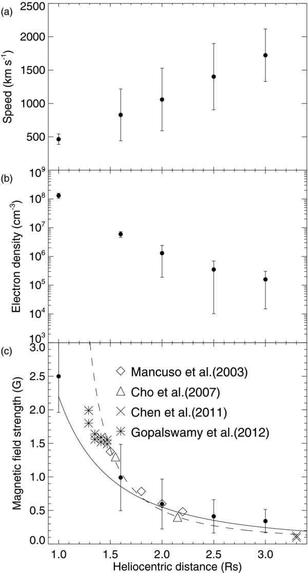
Figure 9. Speeds of coronal disturbance, electron densities, and magnetic field strengths at heliocentric distances of 1.0, 1.6, 2.0, 2.5, and 3.0 R☉. In panel (a), closed circles refer to the average speeds over the traced trajectories of the coronal disturbance at the heliocentric distances, and error bars denote their standard deviations. Panel (b) shows average electron densities and standard deviations with closed circles and error bars (see Appendix B). In panel (c), determined magnetic field strengths are represented by closed circles. Error bars refer to propagating error (Bevington & Robinson 1992) due to the variation of the speed δvf, the uncertainty in sound speed δcs, and the variation of electron density δρ (see Appendix C). Solid and dashed curves show magnetic field strengths found empirically above the quiet-Sun (Mann et al. 1999) and above active regions (Dulk & McLean 1978), respectively.
Download figure:
Standard image High-resolution image3.4. Physical Implication
The COR1 disturbance may be the observational evidence for the fast-mode wave-packets traveling in the extended solar corona discussed by Uchida (1968), who was first to suggest the relation between fast magnetosonic waves and Moreton waves. In addition, the disturbance may have the dome-shaped wave front traveling in the extended corona shown by Afanasyev & Uralov (2011), Grechnev et al. (2011a, 2011b), and Selwa et al. (2012). Because the Alfvén speed increases with height until ∼4 R☉ (e.g., Gopalswamy et al. 2001), wave fronts propagating in all directions at this height range tend to refract toward the solar surface. This physical picture is consistent with COR1 observations of the COR1 disturbance propagating azimuthally in the extended solar corona, with local fast magnetosonic speeds in the range 829–1723 km s−1 varying with the heliocentric distance from 1.6 to 3.0 R☉. Furthermore, the COR1 disturbance turns out to be the upper coronal counterpart of the EUV disturbance propagating against the solar coronal disk traveling with a speed of 465 km s−1, which is much slower than the measured COR1 disturbance. In this context, the COR1 disturbance may be the single wave/shock front that possibly generates the various shock wave signatures in the different solar atmospheric layers simultaneously, such as Moreton waves in the chromosphere, EUV waves in the low corona, and type II radio bursts in the extended corona (Uchida 1968; Klassen et al. 2000; Afanasyev & Uralov 2011; Grechnev et al. 2011a, 2011b; Asai et al. 2012).
The speeds of the COR1 disturbance are consistent with previous measurements by Cheng et al. (2012). Cheng et al. (2012) found a propagating diffuse disturbance decoupled from a CME's lateral flank using COR1 observations on 2011 June 7, and they concluded that the disturbance is in fact a fast magnetosonic wave driven by an expanding CME bubble. This may be the COR1 disturbance we show in this work. They measured the speed of the front at heliocentric distances of 1.95, 2.05, and 2.15 R☉, and the peak speeds are 830 ± 43, 880 ± 27, and 960 ± 48 km s−1, respectively. These values are comparable with what we found, 1059 ± 469 km s−1 at 2.0 R☉. In addition, the speeds tend to increase with heliocentric distance. This tendency may be general in the inner solar corona, as expected from empirical and theoretical models (e.g., Gopalswamy et al. 2001), and may be the key to understanding why the chromospheric and coronal disturbances such as Moreton and EUV waves can appear far away from the flare sites. If a disturbance occurs at a flare site, i.e., a CME, then fast magnetosonic waves can be triggered to propagate in all directions into the corona, most efficiently in the direction normal to the magnetic field lines, and refracted toward the solar surface due to the faster local fast magnetosonic wave speeds in the upper solar corona. This refraction may be the reason that the wave energy reaches distant sites where Moreton and EUV waves are observed.
4. SUMMARY AND CONCLUSION
Using STEREO/SECCHI/EUVI and COR1 observations, we report observations of a fast magnetosonic wave in the solar corona and show that what appear as fronts on the inhomogeneous solar surface can be attributed to the passage of the fast magnetosonic wave in the upper corona. The density compressions propagate globally across open magnetic field lines with local fast magnetosonic speeds ranging from 829 to 1723 km s−1 within the heliocentric distance range of 1.6–3.0 R☉. Furthermore, the disturbance passes through streamer regions known as magnetic separatrices. This wave is found to be the counterpart of the EUV disturbance traveling against the solar coronal disk, known as EIT waves, whose physical nature has been highly debated. As for the stationary fronts, which have been considered as crucial counterevidence for the wave interpretations of EUV disturbance, our observational results indicate that they are not stopping fronts but rather are crucial evidence for the existence of trapped fast magnetosonic waves in streamers sweeping through magnetic separatrices. For these reasons, we conclude that COR1 and EUV disturbances (EIT waves) are in fact fast magnetosonic (fast-mode MHD) waves in the solar corona.
We are grateful to the referee for a number of constructive comments that helped to improve the manuscript. R.-Y.K. and L.O. acknowledge support by NASA grant NNX10AN10G. L.O. also acknowledges support by NASA grants NNX09AG10G and NNX11AO68G.
APPENDIX A: CONE MODEL
The purpose of modeling the three-dimensional structure of the COR1 disturbance is to estimate the footpoint's location of the COR1 disturbance and compare it with the location of the EUV disturbance. To do this, we postulate a cone shape for the expanding COR1 disturbance (motivated by the cone model used to describe CME expansion; e.g., Zhao et al. 2002; Xie et al. 2004). Supposing that the COR1 disturbance is a fast magnetosonic wave propagating in all directions, the shape of the expanding front could be approximated to a sphere or ellipsoid (Patsourakos et al. 2009). The COR1 images may show only a small part of the sphere or ellipsoid, and the part may be represented by a cone of which the vertex is located at the solar center and the axis is passing through the flare site. Solid lines in Figures 1(b), (f), and (j) refer to the axis of the cone. Adjusting the central angle between the axis and the surface of the cone, we find the cone's surface, which fits both fronts of the COR1 disturbance observed by COR1 Ahead and Behind. Concentric circles in Figures 1(b), (f), and (j) represent the cone's surface at heliocentric distances from 1.0 to 5.5 R☉ in intervals of 0.5 R☉.
APPENDIX B: ELECTRON DENSITY
We determine three-dimensional electron density with a tomographic reconstruction method (Kramar et al. 2009) using data taken from STEREO/SECCHI/EUVI Ahead and COR1 Behind. We set data cubes (150, 150, 150) for EUVI and (128, 128, 128) for COR1 to reconstruct the three-dimensional electron density using half a solar rotation before the event occurred on 2011 August 4. Figure 10 shows spherical cross sections of the reconstructed electron density from the COR1 data set, at heliocentric distances 2.0 (top), 2.5 (middle), and 3.0 R☉ (bottom). In order to obtain the radial electron density profile from the data cubes, we take the averages and standard deviations of electron densities in heliocentric distance ranges within ±0.05 at 1.2 R☉ from EUVI and 1.9–3.8 R☉ from COR1 in intervals of 0.1 R☉. Figure 11(a) shows a number distribution of electron density in the heliocentric distance range 2.5 ± 0.05 R☉ with a bin size of 104 cm−3. Because of dense regions as seen in Figure 10, the histogram has a broad tail toward a high-density value. In Figure 11(a), μr and σr with arrows represent the average and standard deviation of the electron density in this range. Open circles and dashed error bars in Figure 11(b) represent μr ± σr in the heliocentric distance ranges.
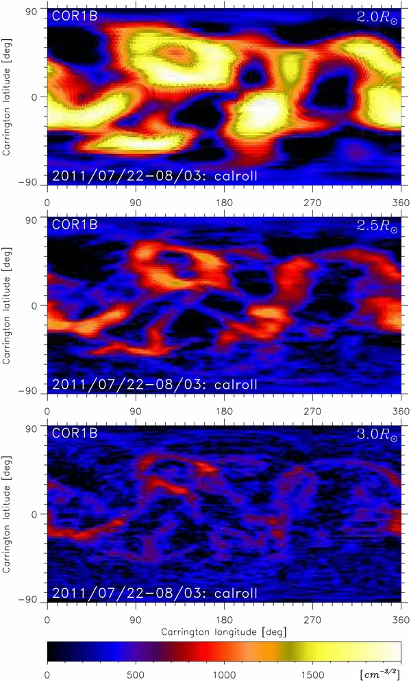
Figure 10. Spherical cross sections of the reconstructed electron density at heliocentric distances 2.0 (top), 2.5 (middle), and 3.0 R☉ (bottom). Three-dimensional electron density in the solar corona is measured by a tomographic reconstruction (Kramar et al. 2009) using the STEREO COR1 Behind data set taken from 2011 July 22 to August 3 before the event occurred on 2011 August 4.
Download figure:
Standard image High-resolution image
Figure 11. (a) Number distribution of the electron density in 2.5 ± 0.05 R☉ with bin size of 104 cm−3 taken from three-dimensional electron density as seen in Figure 10 (middle). μr and σr refer to the average and standard deviation of the electron density in this heliocentric distance range. (b) Open circles and dashed error bars denote average μr and standard deviations σr of measured electron densities at the corresponding heliocentric distances in x-axis within ±0.05 R☉. These values are modeled with a power law in Equation (B1). Solid curve represents the fitting result. Closed circles refer to the values determined by the model fitting at heliocentric distances of 1.0 and 1.6 R☉. The errors in electron densities at these heliocentric distances are defined as standard deviations of measured electron densities at 1.2 and 1.9 R☉ instead of the errors determined by the model fitting. Dashed curve shows the electron density profile found by Leblanc et al. (1998).
Download figure:
Standard image High-resolution image
The electron density profile is modeled with a power law that is appropriate for the low solar corona (Leblanc et al. 1998) as follows:

where r is the heliocentric distance in units of solar radius (R☉) and a, b, and c are free parameters to be determined. Using least-squares fitting, we find electron densities at heliocentric distances of 1.0 and 1.6 R☉ and take standard deviations at 1.2 and 1.9 R☉ as the errors at these heliocentric distances. The χ-square value of this fitting was 0.13. The solid and dashed curves in Figure 11 denote the radial electron density profile found by this work and Leblanc et al. (1998), respectively.
In order to find the mass density profile along heliocentric distance ρ(r), we assume 10% helium in the coronal medium. The mass density is assumed to vary only with height, and the latitudinal variation is neglected.
APPENDIX C: CORONAL SEISMOLOGY
The speed of the fast magnetosonic wave is given by the combination of the local Alfvén speed vA = B/(4πρ)1/2 and the local sound speed cs = (γP/ρ)1/2, where B, ρ, P, and γ are magnetic field strength, mass density of plasma, plasma pressure, and adiabatic index, respectively. The speed in the linear approximation in a homogeneous medium is given by
where vf and θ are the speed of the fast magnetosonic wave and the angle between wave and magnetic field vectors, respectively. Here we postulate that all wakes of the propagating disturbance are purely perpendicular to the magnetic field lines that are parallel to each other, and we neglect any possible effects of structures across the fields on the wave phase speeds. As a result, the speed is reduced to the following expression:

From Equation (C2), the magnetic field strength B can be found by the following relation (in cgs units):
As for the sound speed cs estimate, we simply assume fully ionized ideal gas with a temperature of (1.5 ± 0.5) × 106 K and an adiabatic index of γ = 1, which is close to the value deduced from Hinode observations by Van Doorsselaere et al. (2011). As a result, we find a sound speed of 155 ± 27 km s−1. The error in magnetic field strength is a propagating error due to the uncertainties in the determined disturbance speeds δvf, sound speed δcs, and electron density δne.