


ABSTRACT
The damped random walk (DRW) model is increasingly used to model the variability in quasar optical light curves, but it is still uncertain whether the DRW model provides an adequate description of quasar optical variability across all timescales. Using a sample of OGLE quasar light curves, we consider four modifications to the DRW model by introducing additional parameters into the covariance function to search for deviations from the DRW model on both short and long timescales. We find good agreement with the DRW model on timescales that are well sampled by the data (from a month to a few years), possibly with some intrinsic scatter in the additional parameters, but this conclusion depends on the statistical test employed and is sensitive to whether the estimates of the photometric errors are correct to within ∼10%. On very short timescales (below a few months), we see some evidence of the existence of a cutoff below which the correlation is stronger than the DRW model, echoing the recent finding of Mushotzky et al. using quasar light curves from Kepler. On very long timescales (>a few years), the light curves do not constrain models well, but are consistent with the DRW model.
Export citation and abstract BibTeX RIS
1. INTRODUCTION
The optical variability of quasars has long been a proposed diagnostic of the central engines of quasars (e.g., Kawaguchi et al. 1998). While the physical origins of variability remain an open question (see, e.g., Dexter & Agol 2011), recently it has been proposed that the optical variability of quasars is mathematically well described by a damped random walk (DRW; Kelly et al. 2009), which characterizes quasar light curves as a stochastic process with an exponential covariance function S(Δt) = σ2exp (− |Δt/τ|), defined by an amplitude σ and a characteristic timescale τ. Kelly et al. (2009), Kozłowski et al. (2010), and MacLeod et al. (2010) have shown that the DRW model provides a viable explanation for the variability of individual quasars found in a heterogeneous sample, Optical Gravitational Lensing Experiment (OGLE; Udalski et al. 1997) and the Sloan Digital Sky Survey (SDSS) Stripe 82 (S82; Sesar et al. 2007), respectively, and that the parameters τ and σ are correlated with the physical properties of the quasar (rest wavelength, luminosity, and black hole mass). MacLeod et al. (2011) also demonstrated that the ensemble structure functions (SFs) of quasars can be recovered by modeling each individual quasar with a DRW based on its luminosity, rest wavelength, and estimated black hole mass.
The DRW model is also a powerful tool. For example, it provides a well-defined approach to variability-selecting quasars (Kozłowski et al. 2010; MacLeod et al. 2012; Butler & Bloom 2011). It also provides a well-defined approach to interpolating and modeling quasar light curves in reverberation mapping studies. Zu et al. (2011) show how it provides a general approach to measuring lags in one or more emission lines or velocity bins of a single line. The model has been used by Grier et al. (2012), and a variant was used by Pancoast et al. (2011).
However, it is still uncertain whether the DRW model, with only two parameters, can fully characterize quasar optical variability across all timescales. Early studies (e.g., Collier & Peterson 2001) examined the power spectrum density (PSD) of a small number of individual quasars, finding evidence for the f−2 power-law behavior of the DRW model on short timescales, and weaker evidence for a flattening on long timescales. The first series of DRW studies (Kelly et al. 2009; Kozłowski et al. 2010; MacLeod et al. 2010) essentially followed these results and reconfirmed the average PSD structure, but did not explore any possible deviations. We know from Mushotzky et al. (2011) that the DRW model probably fails on very short timescales (≲week), having too much power on short timescales compared to that measured by Kepler. Mathematically speaking, the DRW model (a.k.a. the Ornstein–Uhlenbeck process) is unique—it is the only stationary Gaussian process (GP) that is "memoryless" (Markov). Kelly et al. (2009) introduced the DRW model as a first-order continuous autoregressive (CAR(1)) process, and its discrete counterpart (AR(1)) is simply an iteration xi + 1 = αARxi +  i, where is a Gaussian deviate.4 Physically, if quasar variability is driven by multiple mechanisms, or multiple seeds of the same mechanism with different relaxation timescales or amplitudes, there should be deviations from the DRW model.
Traditional quasar variability studies often rely on examining the PSD (or the SF as its real space equivalent) of the light curves. PSD-based methods have two major drawbacks: one in measurement and one in interpretation. In particular, the measurement of the PSD requires binning the light curves, which are generally irregularly sampled for various reasons (weather, observing seasons, etc.). Information is always lost by binning. More importantly, the uncertainties between the binned points are very strongly correlated, making any statistical interpretation difficult without correctly estimating the covariance matrix. While it is possible to reconstruct the full covariance matrix of the empirical PSD using Monte Carlo methods (e.g., Uttley et al. 2002), in this study we simply build a statistical model of the light curve as a GP in the time domain, where no discretization of data is involved, and it is easy to include all the model/data covariances. This makes our approach more statistically powerful than turning the light curve into an estimate of the PSD and then fitting a model to the estimated PSD at the minor price of never producing a visually appealing picture of the PSD (or SF).
In this paper, we explore several alternative covariance functions with a third parameter that allows for deviations from the DRW model and explore whether they provide a better representation of quasar variability. This needs to be done for individual quasars because we are now certain that the ensemble statistics (e.g., SFs) of quasars are weighted averages of individual quasars with different individual statistics (MacLeod et al. 2012). We employ the OGLE light curves of quasars behind the Small and the Large Magellanic Cloud (SMC and LMC). Thanks to the high cadence and long baseline of OGLE, the light curves generally have ∼570 photometric epochs over ∼7 yr, making them extremely well suited for studies of quasar variability. We describe this data set and our sample selection in Section 2. In Section 3 we introduce four new covariance functions that we use to test for deviations from the DRW model and describe the model fitting procedures. We present our main results in Section 4. We conclude by discussing the physical implications in Section 5.
2. OGLE QUASAR LIGHT CURVES
We use the light curves of quasars behind the LMC and SMC monitored by OGLE (Udalski et al. 1997, 2008). Most of these were identified by Kozłowski et al. (2011, 2012) in part from candidates variability-selected using the DRW model (Kozłowski et al. 2010). The photometric uncertainties of the light curves were estimated by using Difference Image Analysis (DIA; Wozniak 2000). The initial sample consists of 223 I-band quasar light curves. There are typically ∼570 epochs taken over ∼7 yr on a two-day cadence with six-month seasonal gaps when OGLE instead focuses on the Galactic bulge. For comparison, the S82 quasars have only ∼50 epochs nominally over ∼10 years, but there are really a few epochs in 1998, a gap until 2000 with 1–3 epochs per year coverage to 2005, and then 10–30 epochs per year from 2005 to 2008. The OGLE quasars should allow us to investigate quasar variability on both small and long timescales in more detail than the SDSS S82 light curves.
Since we are examining the problem of additional parameters, we need higher quality light curves than if we were only trying to estimate DRW parameters. Starting from the 223 light curves, we first selected sources with high signal-to-noise ratio for their variability, keeping sources where the rms magnitude variation σrms was significantly larger than the mean photometric error σm (σrms/σm > 2.0). We also required σm < 0.1 mag. The typical photometric error for bright stars in OGLE is 0.01 mag, but the typical quasars are relatively fainter and so have larger photometric uncertainties because there are only ∼3 QSOs per square degree at I ⩽19 mag (Richards et al. 2006). This left us with 87 light curves in the sample. Next we required that the light curves yield a well-defined DRW timescale τ by requiring that both  and
and  , where
  ,
,  , and
, and  are the likelihoods for τ = 0, τ = ∞, and the best-fit τ, respectively, where the best-fit τ are in the range of 17 ≲ τ ≲ 2700 days. This is to ensure that the light curves have some statistically detectable characteristic timescale. The final sample has 55 light curves of quasars with redshifts between 0.15 and 2.50 and I-band apparent magnitudes between 16.7 and 19.4 mag.
About 45% of the objects are at redshifts where the I-band continuum variabilities are contaminated by the lagged variabilities of broad emission lines. For a broadband filter like the I band and assuming a typical quasar spectrum (Vanden Berk et al. 2001), the line contributes only ≲ 6% of the flux in the filter (except for two objects at z ∼ 2.45 where the Hα line contributes up to 14% of the I-band flux). Since we are probing the shape of the covariance functions instead of the variability amplitudes, we do not expect this small level of contamination to affect our results. We tested for any effects by dividing our sample into line-contaminated and line-free sub-samples, and found negligible differences between the two sub-samples in the likelihood analyses. Throughout the paper we fit logarithmic light curves (i.e., in magnitudes, as in Kelly et al. 2009; Kozłowski et al. 2010; MacLeod et al. 2010), although we used linear flux scales in Zu et al. (2011). There is currently no theoretical argument favoring fitting on one scale over another. Observationally, when the variability amplitude of quasars is modest, we have found that fitting on log and linear scales gives almost identical results. Since the results seem little affected by either broad line contamination or the scales used in fitting, we will not discuss these issues further.
3. COVARIANCE FUNCTIONS AND ANALYSIS METHOD
We model each light curve as a GP,5 defined by a covariance function S(Δt) = cov(m(t), m(t + Δt)) where Δt is the time separating two observations and we assume a stationary process with a well-defined mean. The covariance function is related to the SF by

and to the PSD by a Fourier transform

In particular, the DRW model has a covariance function of
and a PSD of
We do not repeat the SFs of the individual models because they are trivially related to the covariance functions (Equation (1)). The DRW model can be equivalently parameterized by τ and the asymptotic amplitude of the SF( ; MacLeod et al. 2010), or τ and the slope of the SF on short timescales (
 ; Kelly et al. 2009).
We consider the four modified covariance functions shown in Figure 1. A natural variant of the DRW covariance function is the so-called powered-exponential (PE) function (Neal 1997)
where the special case γ = 1 corresponds to the DRW model. The PSD for the PE covariance can be expressed in a closed form only for γ = 1 (DRW) and 2 (Gaussian), but for small timescales (s → ∞), P(s)∝s−(γ + 1) (Lim & Muniandy 2003). The PE model modifies the DRW model on both long and small scales (panel (a) of Figure 1) and is the model used in Pancoast et al. (2011).
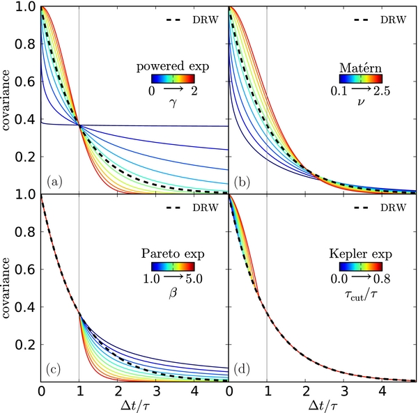
Figure 1. Comparison of the powered-exponential (panel (a)), Matérn (panel (b)), Pareto-exponential (panel (c)), and Kepler-exponential (panel (d)) covariance functions (thin solid curves) with the DRW model (thick dashed curves). The third parameter of each model is given by the gray-scale color bar in each panel. The models are normalized to unity at zero lag.
Download figure:
Standard image High-resolution imageThe "Matérn" (MA) covariance function (Matérn 1960) is defined by
where Γ is the gamma function, Kν is a modified Bessel function of the second kind, and the new parameter, ν, primarily adjusts the correlation function on short timescales (ν > 0). The covariance function is exponential on long timescales  as Δt → ∞. The MA covariance function has a PSD (Abramowitz & Stegun 1965) of
The special case ν = 0.5 gives the DRW covariance function (panel (b) of Figure 1).
Mushotzky et al. (2011) found that the quasar light curves measured by Kepler do deviate from the DRW model on very short timescales (∼days) with steeper PSD power-law slopes of −2.6 to −3.3, rather than the −2 of the DRW model (Equation (4)). Thus, there must be a τcut below which the fluctuation amplitudes cut off more sharply than in the DRW model. The OGLE light curves, with a typical cadence of ∼2 days, overlap the timescales of the Kepler light curves (∼6 hr to ∼1 month), so there is some prospect of searching for a short timescale cutoff. To search for the cutoff within our sample light curves, we define the Kepler-exponential (KE) covariance function by modifying the DRW model on very short timescales to be
where τcut is the cutoff timescale below which the covariance function is stronger than the DRW model, so that the PSD has a similarly steep slope as found for the Kepler light curves. The model returns to the DRW model for τcut = 0 (panel (d) of Figure 1), although we should not be able to recognize values of τcut on scales smaller than a few times the typical cadence (∼10 days).
In order to test for deviations from the DRW on long timescales, we combined the DRW model on short timescales with the "Pareto" function (Pareto 1967) on long timescales (the "Pareto exponential," PA),
where the power-law index α > 1 controls the extent of the covariance tails (panel (c) of Figure 1). In this case, no value of α exactly matches the DRW and placing the break at timescale τ is reasonable but arbitrary.
Our goal is simply to estimate a value for the new parameters introduced in each of these models using a maximum likelihood (ML) approach. We briefly recap the components of the likelihood function here and refer readers to Zu et al. (2011), Kozłowski et al. (2010), and Rybicki & Press (1992) for details. We model each light curve as

where s(t) is the underlying variability signal with covariance matrix S,6 n is the measurement uncertainty with covariance matrix N, L is a vector with all elements equal to one, and q is the light-curve mean.7 After optimizing the value of q, the likelihood of the model parameters is
where C is the overall data covariance S+N and

This approach needs no binning of the data and automatically includes all the data and model uncertainty covariances, making it broadly superior (in a statistical sense) to standard uses of the PSD or SF.
We first fit each quasar light curve with the DRW model to obtain ML estimates for σ and τ, which are then used to generate a mock light curve that is fully consistent with the DRW model while having exactly the same time sampling and photometric uncertainties as the true light curve. We generate the DRW mock light curves as random GP realizations using the Cholesky decomposition method described in Zu et al. (2011), which is a generic method for all covariance function models. DRW mock light curves can also be easily generated as CAR(1) processes (see footnote 4; Kelly et al. (2009)). Finally, we add a Gaussian deviate normalized by the estimated photometric error of each data point to incorporate the measurement uncertainties of the data into the mock light curves. We use these mock DRW light curves as a comparison sample when evaluating the evidence for any additional parameters.
Next, we fit both the data and the mock light curves using each of the four covariance functions. Since we only care about the differences in the third parameter, we start with an ML analysis based on ![$\mathcal {L}(\rm{[\gamma , \nu , \tau _\mathrm{cut}, \alpha ]})\equiv \mathcal {L}(\tau _{\max }, \sigma _{\max }, \rm{[\gamma , \nu , \tau _\mathrm{cut}, \alpha ]})$](https://content.cld.iop.org/journals/0004-637X/765/2/106/revision1/apj460809ieqn11.gif) where τmax and σmax maximize the likelihood at fixed third parameter for each light curve. In addition to considering the models of the individual light curves, which we will refer to as the individual models, we also want to derive the mean and dispersion of the third parameter of each model for the ensemble light curves. However, since the individual likelihoods are mostly asymmetric with non-Gaussian tails, it is inappropriate to calculate the weighted mean directly from the best-fit third parameters of individual models. To fully take into account the shape of individual likelihoods, we multiply (add) all the individual (log)likelihood functions together to obtain a "combined" likelihood function of the third parameter. By comparing the "combined" and individual likelihood functions for the data and mock light curves, we can then assess how significant the best-fit third parameter deviates from or agrees with the DRW prediction in each of the four modifications. We will focus on this as a problem of parameter estimation rather than model testing, although we will discuss model testing.
where τmax and σmax maximize the likelihood at fixed third parameter for each light curve. In addition to considering the models of the individual light curves, which we will refer to as the individual models, we also want to derive the mean and dispersion of the third parameter of each model for the ensemble light curves. However, since the individual likelihoods are mostly asymmetric with non-Gaussian tails, it is inappropriate to calculate the weighted mean directly from the best-fit third parameters of individual models. To fully take into account the shape of individual likelihoods, we multiply (add) all the individual (log)likelihood functions together to obtain a "combined" likelihood function of the third parameter. By comparing the "combined" and individual likelihood functions for the data and mock light curves, we can then assess how significant the best-fit third parameter deviates from or agrees with the DRW prediction in each of the four modifications. We will focus on this as a problem of parameter estimation rather than model testing, although we will discuss model testing.
4. RESULTS
The results of our model depend on how well the DIA photometric errors of the light curves in our sample are determined. Assuming that the DRW is an adequate model for each individual light curve,8 we can estimate the fractional errors in the photometric error estimates from the χ2/dof distribution of the DRW fits to the 55 light curves. For all these objects, the overall goodness of fits to the light curves with the DRW model are reasonable (0.88 < χ2/dof < 1.53), with an average 〈χ2/dof〉 ≃ 1.09 and dispersion  , while we would expect 〈χ2/dof〉 = 1 and
  . These differences could be explained by fractional shifts σm = σtruem(1 + e) between the true uncertainties σtruem and the nominal error bar σm where the mean fractional error is 〈e〉 = −0.04 with a dispersion of σe = 0.06. This simple assumption on the OGLE photometric uncertainties will help us understand the scatter in any additional model parameter between quasars, but to cover all the possibilities, we discuss the implications of our results in terms of two scenarios: (1) that the OGLE photometric uncertainties are correct to high accuracy (∼10%) and lack significant non-Gaussian tails, (2) that the uncertainties are slightly underestimated and/or have some non-Gaussian tails. We hereby refer to the two scenarios as case I and case II, respectively.
We simply discuss each of the four models in turn, starting with the PE model results shown in Figure 2. The panels on the left show that the combined results, where we merge the likelihood functions of all 55 quasars, agree with the DRW model remarkably well. The joint marginal likelihood function for γ strongly peaks near γ = 1.0 with 〈γdata〉 = 0.98 ± 0.04 using  for the error estimate (which would correspond to 2σ for Gaussian uncertainties). This is generally consistent with the result for the mock light curves of 〈γmock〉 = 1.04 ± 0.03. The individual likelihoods, shown in the right panels of Figure 2, seem to show a larger scatter in the data (σγ, data = 0.37) than in the mock data (σγ, mock = 0.19). While essentially all the light curves are consistent with the DRW at better than 3σ (
 ), there is one extreme outlier (seen as the spike at γ = 0.14). While there is nothing obviously odd in this object's light curve, it is very close to our noise selection limit and a source will be biased toward low γ (closer to white noise) if the true measurement errors are larger than estimated (see below). This object is also an outlier in the other models. Nonetheless, excluding or including it has a negligible effect on the combined likelihood functions.
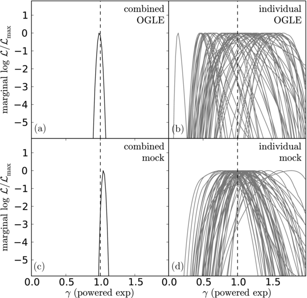
Figure 2. Combined (left panels: (a) and (c)) and individual (right panels: (b) and (d)) marginal log-likelihoods for γ in the powered-exponential model for the data (top panels: (a) and (b)) and the mock data (bottom panels: (c) and (d)). The combined results are the sums of the log-likelihoods of the individual quasars. For the DRW model γ = 1.0, as indicated by the vertical dashed line.
Download figure:
Standard image High-resolution imageBefore going to other models, we want to interpret the larger spread we observe in the best-fit γ for the individual data light curves (panel (b) of Figure 2). The difference of the dispersions between the individual best fits in the data and mock light curves is σγ = (σ2γ, data − σγ, mock)1/2 = 0.31 (0.29 if we drop the one extreme outlier). This can be interpreted either as evidence for intrinsic scatter if case I is correct, or as evidence for problems in the photometric uncertainties σm (case II). As an experiment, we refit the PE model to the mock light curves after resetting σm to be 20% larger (e = +0.2) or smaller (e = −0.2) than the actual uncertainties used to generate the mock light curves. The results of the experiment are shown in Figure 3. When the noise is overestimated, true variability power on short timescales is instead interpreted as noise, so the models shift to higher γ for stronger correlations on short timescales. When the noise is underestimated, noise on short timescales is interpreted as signal, so the models shift to lower γ for weaker correlations. As expected, in Figure 3, overestimating the errors biases the estimates of γ to be high, with 〈γ+mock〉 = 1.30 ± 0.04 (panel (a) of Figure 3), and vice versa when underestimating errors, 〈γ−mock〉 = 0.62 ± 0.01 (panel (c) of Figure 3). Given that a 20% error in σm causes a 0.3 bias in the estimate of γ, so that γ ≃ 1 + 1.5e, then the excess variance in the estimates of γ for the data could be explained by making σe = 0.20, which is significantly larger than the σe = 0.06 suggested by the χ2/dof distribution. Also note that the estimate of 〈e〉 from the χ2/dof distribution would tend to shift the estimates of γ for a DRW model to γ = 1 + 1.5〈e〉 ≃ 0.93, so systematic uncertainties in the photometric errors produce uncertainties comparable to the statistical uncertainties in 〈γ〉. If we use σe = 0.06 from the χ2/dof distribution as an estimate of the scatter in the fractional uncertainties in σm (case I), then we appear to be left with σinγ = 0.28 of intrinsic scatter between quasars. If case II is correct (i.e., σe ∼ 20% or strong non-Gaussian tails in σm), the observed mean and spread of γ are consistent with DRW model with little quasar-to-quasar variation.
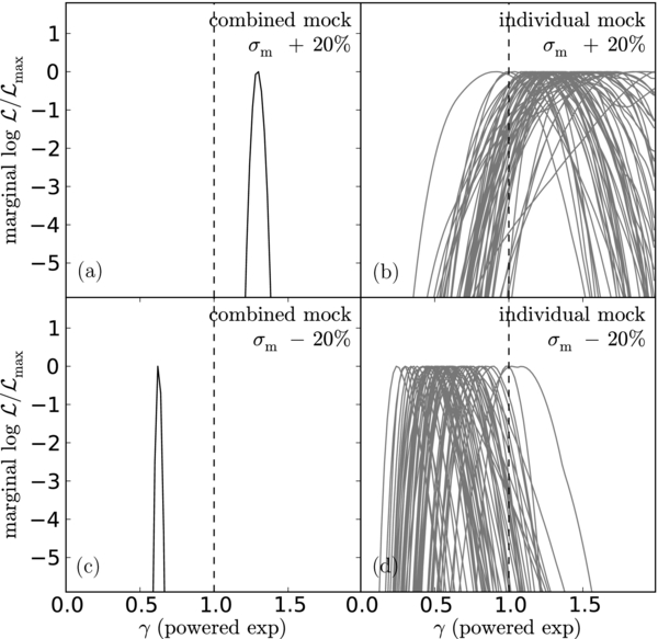
Figure 3. Effects of incorrect error estimates for the powered-exponential model. The top (bottom) panels assume that the true photometric errors are over (under) estimated by 20%. As in Figure 2, the left (right) panels show the joint (individual) estimate of the new parameter γ. The effects of misestimating the photometric errors are qualitatively similar for the other three models.
Download figure:
Standard image High-resolution imageFor two other models (MA and PA, discussed further below), we also see evidence for larger spread in the best-fit third parameter in the data than in the mock data. We have done similar experiments of scaling the photometric uncertainties for each model and the results stay consistent with our findings for the PE model and the two possible interpretations. To avoid unnecessary repetition, we will only report the intrinsic scatters inferred from each experiment for the two models.
Figure 4 shows the results for the MA model. The likelihood function for the data is again strongly peaked at the value that corresponds to the DRW model, ν = 0.5, with 〈νdata〉 = 0.492 ± 0.016, as compared to 〈νmock〉 = 0.525 ± 0.017. The distribution of the individual results is again broader for the real data than for the mock data, suggesting an excess scatter of σν = 0.08 in ν if there are no other systematic uncertainties. In this case, the sensitivity to the uncertainties in the photometric errors is ν = 0.5 + 1.1e, suggesting an intrinsic scatter of σinν = 0.05 in case I and broad consistency with DRW model in case II.
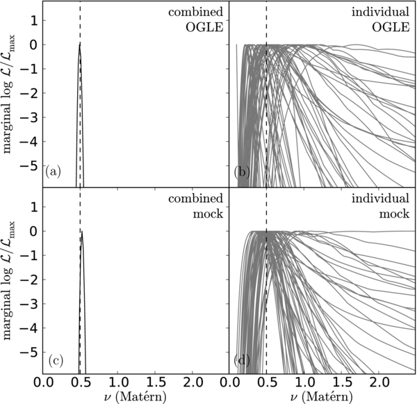
Figure 4. Same as in Figure 2 but for the Matérn model. Here ν = 0.5 corresponds to the DRW model.
Download figure:
Standard image High-resolution imageOn even shorter timescales, the histograms in Figure 5 show the distributions of the best-fit τcut of the KE model for the data (left panel) and the mock (right panel) light curves. For the data, there is a clearly bimodal distribution of τcut demarcated by a gap around 10 days that corresponds to five times the typical cadence (2 days). The first peak below 10 days comprises objects that are either consistent with the DRW model (τcut = 0) or have a τcut that is unresolved by the OGLE sampling (⩽4 discrete values of Δt below τcut could be computed for SKE in Equation (8)). The second peak at 30–100 days is well beyond the cadence scale, indicating another population of objects (23 out of 55) that favor a cutoff timescale beyond a month. For the mock sample, there is only a single peak below 10 days and a steady decrease toward longer τcut, with only 11 out of 55 objects having τcut larger than a month. Unfortunately, the estimates of τcut are very susceptible to errors in the estimated photometric errors, so the second peak in the τcut distribution of the data light curves could also be an artifact of the scatter in e. Thus, a cutoff timescale τcut ∼ 1–3 months may be marginally detected in half of the quasars, but the cadence and photometric uncertainties of the data are not optimal for probing this regime.

Figure 5. Distribution of quasars as a function of the best-fit τcut for the data (left panel) and mock (right panel) light curves using the Kepler-exponential model. The vertical dashed line in each panel at 10 days indicates the scale below which no variability signal can be resolved for the lack of sampling the Kepler-exponential covariance function below τcut.
Download figure:
Standard image High-resolution imageSince the DRW model is a restricted form of the PE, MA, and KE models, with γ = 1, ν = 0.5, and τcut = 0, respectively, we could use a standard  -test to evaluate whether the DRW model is preferred. We must simply treat the matrix determinant in the likelihood (Equation (11)) as an additional contribution to the χ2, so
  . If we adopt a probability threshold of p > 5%, 50 (PE), 51 (MA), and 53 (KE) out of 55 mock light curves are consistent with the null hypothesis that no additional parameter is needed. For the real light curves, 34, 33, and 53 of the 55 light curves have p > 0.05 for the PE, MA, and KE models, respectively. Thus we again find that the light curves are generally consistent with the DRW model but with some scatter about it. The problem, however, is that the
  -test is not truly applicable to the likelihood computed in Equation (11). A more appropriate approach is to compare the three models using a Bayesian framework. In this approach, the addition of parameters is penalized by modifying the likelihood. Two standards are the Bayesian information criteria (BIC; log L − 0.5klog n, where k and n are the numbers of model parameters and data points, respectively) and the Akaike information criteria (AIC; log L − k). The two criteria are very similar, except that the BIC more heavily penalizes the addition of parameters. The DRW model is overwhelmingly favored by the more "conservative" BIC, while for the more "liberal" AIC, the probability ratios are PDRW: PPE: PMA = 2: 1: 1.
Finally, the light curves do not constrain changes in the structure of covariance function on longer timescales. The individual likelihood functions for α in the PA model are mostly flat, as shown in Figure 6. The combined constraint from the data favors a slightly higher value of 〈αdata〉 = 3.38 ± 0.45 than the mock light curves, 〈αmock〉 = 2.83 ± 0.42, but the two peaks are mutually consistent. The uncertainties are, however, too large to justify additional models for the long timescale behaviors.
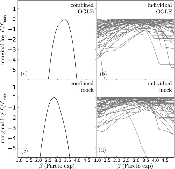
Figure 6. Same as in Figure 2 but for the Pareto-exponential model. No value of β corresponds to the DRW model.
Download figure:
Standard image High-resolution image5. DISCUSSION
We considered four families of covariance functions to test whether there is any evidence that quasar optical variability differs from a DRW model on timescales of weeks to years. Our conclusion is that deviations may exist, but they are small enough that we are reluctant to draw a firm conclusion. The significance of the deviations is very sensitive to the accuracy of the photometric errors, and different tests lead to different statistical conclusions.  -tests, which are not really correct given our likelihood functions, imply that the differences are real, while Bayesian methods, which are more applicable, imply that the modifications are unnecessary or only equally probable as compared to the default DRW model, depending on the information criterion used to evaluate the question. Thus, we will discuss the results in terms of both possibilities. More specifically,
- 1.on the timescales best sampled by the light curves (from months to years), the typical light curve is generally well described by the DRW model, potentially with some intrinsic scatter in the true structure of the power spectrum if the photometric error estimates are correct to better than 10%. The observed scatter could also be extrinsic if the uncertainties in photometric error estimates are larger than 10% or the error distributions have non-Gaussian tails.
- 2.on very short timescales, there are hints of a characteristic cutoff timescale τcut (1–3 months) for ∼50% of the quasars, below which the correlations become stronger than predicted by the DRW model. This is consistent with the Kepler results of Mushotzky et al. (2011), but the OGLE data are clearly not competitive with Kepler in this regime.
- 3.on very long timescales, the light curves are consistent with the DRW model, but the precision of the test is limited by the length (seven years) of the light curves.
Under the assumption that the photometric error estimates are broadly correct to with 10%, the apparent scatter about the DRW model may well be evidence for multiple stochastic processes rather than a single DRW. For example, the PE covariance function can be viewed as the mixture of a continuous sum of independent DRW models with characteristic timescale τi,
where s ≡ τi/τ, σ2(sτ) is the amplitude of process i, and P(s, γ) is the probability density function for the process on timescales τ. The combination of P(s, γ)σ2(sτ) is then the inverse Laplace transform of the PE (Johnston 2006). For γ = 1 (DRW), P(s, γ) is a Dirac δ function at s = 1, so there is only one process operating at one timescale τ. Adding several weaker processes with different timescales would then appear as a scatter about γ = 1, but would be difficult to distinguish from a single DRW model. This is similar in spirit with the work of Kelly et al. (2011), where they modeled quasar optical variability as a linear mixture of different DRW processes and found that it generally provides no better fit than a single DRW model. In the toy model adopted by Dexter & Agol (2011), they matched the observed DRW variability by exciting many independent fluctuating zones with exactly the same τ = 200 days in the accretion disc, and then argued that the resulting change in the effective temperature profile of the disk would explain the observed discrepancies between thin disc sizes inferred from gravitational microlensing of lensed quasars and their optical luminosities (Morgan et al. 2010).
It would be useful to have occasional campaigns in which OGLE sampled shorter timescales with longer integration times to fill in these time baselines with higher precision data. On long timescales, the OGLE-IV project is already extending the light curves, so it will become increasingly possible to explore the long timescale behavior of individual quasars. As the behavior on long timescales (decades) becomes better constrained, it will also be easier to constrain the short timescales (months to years) because there will be less freedom due to covariances between the parameters. The continuing spectroscopic surveys by Kozłowski et al. (2012) will also greatly increase the number of confirmed quasars with OGLE light curves. DES (The Dark Energy Survey Collaboration 2005), LSST (Ivezic et al. 2008), and Pan-STARRS (Kaiser et al. 2002) will carry out similar extensions for the SDSS S82 quasars but generally at lower cadence (albeit for larger numbers of objects). Given a larger sample it will also be possible to search for correlations of the apparent deviations from the DRW model with other physical characteristics of the quasars (luminosity, wavelength, etc.).
C.S.K. is supported by the NSF grant AST-1009756. OGLE is supported by the European Research Council under the European Community's Seventh Framework Programme (FP7/2007-2013), ERC grant agreement No. 246678. S.K. is supported by the Polish Ministry of Science and Higher Education (MNiSW) through the "Iuventus Plus" program, award number IP2010 020470.
Footnotes
- 4
In fact, a DRW light curve is easily generated by using an iterative process with
 and setting the variance of the Gaussian deviate i to be .
 - 5
In principle there could be deviations of light curves from GP, but the impact should be small given the χ2 distribution of the best-fit models (see, e.g., Figure 1 of Zu et al. 2011).
- 6
The entries of Sij are simply the values of the covariance function Sij = S(Δtij), so we have used the same symbol for both.
- 7
The simultaneous fit of q is important because any constant level of contamination (e.g., host galaxy light) is removed by marginalizing over q. Although we are fitting on log scales, to first order the constant flux contribution can be "subtracted" in magnitudes as well.
- 8
The DRW model has one fewer degree of freedom than the other models, so the inferred error statistics should be more conservative.