


ABSTRACT
To understand the behavior of cosmic-ray modulation seen by the two Voyager spacecraft in the region near the termination shock (TS) and in the heliosheath at a distance of >100 AU, a realistic magnetohydrodynamic global heliosphere model is incorporated into our cosmic-ray transport code, so that the detailed effects of the heliospheric boundaries and their plasma/magnetic geometry can be revealed. A number of simulations of cosmic-ray modulation performed with this code result in the following conclusions. (1) Diffusive shock acceleration by the TS can significantly affect the level of cosmic-ray flux and, in particular, its radial gradient profile in the region near the TS and in the inner heliosheath. (2) The radial profile of cosmic-ray flux strongly depends on longitude. There is a slight north–south asymmetry due to an asymmetric TS, but the larger difference in the radial profiles comes from longitudinal variation. Voyager 1 and 2 are separated by ∼ 40° in longitude. Simulations in these two directions show a large difference in the radial profile of cosmic-ray flux. Thus, it is not appropriate to determine the cosmic-ray radial gradient by directly using the two-point Voyager measurements. Various other simulations are also performed to show how sensitively the modulation level depends on latitude, cosmic-ray energy, and interstellar spectrum.
Export citation and abstract BibTeX RIS
1. INTRODUCTION
Records of Galactic cosmic rays obtained by experiments on Earth show that their intensity is anti-correlated with the 11 year solar activity and other solar disturbances. This phenomenon is called solar modulation of cosmic rays. It occurs because when cosmic-ray particles enter into the heliosphere, they encounter the expanding solar wind with a frozen-in magnetic field. The convective motion of the magnetic field can prevent cosmic rays from entering while the expansion of the solar wind causes the particles to lose energy adiabatically, resulting in a reduction of cosmic-ray flux inside the heliosphere. Currently, it is widely accepted that the solar modulation of cosmic rays is due to a combination of effects caused by diffusion and drift in the turbulent interplanetary magnetic fields (IMFs), solar wind convection, and adiabatic cooling (Gleeson & Axford 1968; Jokipii et al. 1977, 1979, 1981; Kota & Jokipii 1983). The theoretical foundation can be summarized by the following transport equation (Parker 1965):

While the basic mechanisms of cosmic-ray modulation are understood, the properties of the solar wind plasma and magnetic field in the entire heliosphere are still not well known enough to yield accurate predictions of cosmic-ray modulation from the Parker transport equation. In particular, the heliosphere is divided into several regions of very different plasma and magnetic properties. The location and geometry of the boundaries that separate these regions will have strong effects on cosmic-ray modulation. For example, the termination shock (TS) slows down the solar wind from a supersonic radially expanding flow to a nearly incompressible hot plasma in the heliosheath. The properties of cosmic-ray transport, such as convection speed and adiabatic cooling rate, change dramatically across the TS. The shock can also accelerate particles, which reverses the effect of adiabatic cooling. In order to understand the effects of heliospheric boundaries, it is essential that numerical cosmic-ray modulation models incorporate accurate plasma and magnetic field structures of the heliosphere. This is required as the Voyager spacecraft are obtaining new measurements of cosmic rays in the heliosheath.
In the past, cosmic-ray modulation models were built based on analytical models of the heliosphere with a uniform solar wind stream and the Parker IMF (Jokipii and his collaborators: Jokipii et al. 1977, 1979, 1981; Kota & Jokipii 1983). These early models were enough to reveal many properties of cosmic-ray modulation in the inner heliosphere because the detailed structure of the heliospheric boundary is of little consequence. Later, it was found that the nearly vanishing magnetic field in the polar region causes some difficulty when calculating diffusion coefficients there. Jokipii proposed a modified Parker IMF (Jokipii & Kota 1989), and this modification was used later in the calculation of cosmic-ray modulation (Caballero-Lopez et al. 2004). Fisk proposed another type of heliospheric magnetic field (Fisk 1996), considering the motion of the magnetic field line footpoint on the Sun. Later, this model was used by Burger & Hitge (2004) to investigate the latitudinal gradient of cosmic-ray modulation. Instead of using these modified magnetic fields, an enhanced perpendicular diffusion coefficient form can also be directly adapted in the polar region (Potgieter 2000). Similarly, after the solar wind speed was found by McComas et al. (2001) to have two types—a fast solar wind from a polar coronal hole and a slow solar wind in the streamer belt—a solar wind model with latitude-dependent speed (Ferreira & Potgieter 2004) was used in the simulation of cosmic-ray modulation in the solar minimum period.
As the Voyager spacecraft move into the outer heliosphere, the effects of the TS and the heliosheath on cosmic rays are more noticeable (Webber & Lockwood 2001). Cosmic-ray modulation models should now incorporate these regions. Potgieter & Moraal (1985), Le Roux & Potgieter (1995), and Ferreira & Potgieter (2004) adapt the same model inside the heliosheath as a supersonic solar wind region, which is not appropriate. Caballero-Lopez et al. (2004) separate the situation inside the heliosheath and supersonic region. They use the form (rs/r)2 to model the solar wind speed variation inside the heliosheath. But none of these methods can correctly reflect the possible complex structures inside the heliosheath, such as the bending heliospheric current sheet, magnetic wall, and so on.
Magnetohydrodynamic (MHD) theory has been widely used to study the interaction between the solar wind and the interstellar medium (ISM). The magnetic field and solar wind speed are derived as the natural solution of a set of MHD equations. One advantage of the MHD heliosphere model is that it can be made as realistic as possible given correct input of ISM plasma and magnetic field parameters. For example, the profile of the interstellar magnetic field (ISMF) can be included so that the model can reveal the effects of external magnetic pressure on the shape and size of heliospheric boundaries such as the TS and heliopause. There are many MHD models of the heliosphere, but creating a complete model is still challenging because correctly treating the interstellar neutral atoms (Pauls et al. 1995, 1996; Baranov et al. 1993; Heerikhuisen et al. 2006; Pogorelov et al. 2009) is not simple. Linde et al. (1998) only consider the continuity equation for interstellar neutral atoms, namely, the mass loading onto the solar wind caused by interstellar neutral atoms. In addition, he did not distinguish between the different types of interstellar neutral distributions. Therefore, the distribution of these atoms remains the same inside the heliosphere. Pogorelov et al. (2008) provided a more realistic treatment of interstellar neutrals based on their kinetic treatment with a stochastic Monte Carlo method proposed by Heerikhuisen et al. (2006), and the ISMF was pointed toward the southern heliosphere at an angle of 30° to the ecliptic plane. As a consequence of these treatments, the TS became less asymmetric and more expanded compared to Linde's MHD model.
Researchers modeling cosmic-ray modulation have begun to take advantage of MHD modeling of the heliosphere. Florinski et al. (2003) and Florinski & Jokipii (1999) used a self-consistent model coupled with the MHD equation and the cosmic-ray transport equation to study cosmic-ray modulation. But their method was confined to two dimensions and the cosmic-ray drift term was not included. Ferreira & Scherer (2006) used a similar self-consistent method to study the time evolution of cosmic-ray spectra. Ball et al. (2005) used an MHD heliosphere model developed by Linde et al. (1998) to study cosmic-ray modulation. Predictions of cosmic-ray intensity along several radial directions were made. This was the first three-dimensional modulation code to be combined with an MHD heliosphere, but the shape of the heliosphere does not correctly match our currently updated knowledge about heliospheric structures. As Voyager 1 and Voyager 2 entered into the heliosheath region separately in 2004 and 2007 (Stone et al. 2005, 2008), the two spacecraft provided direct observational data for the heliospheric boundaries, plasma, and magnetic field parameters in the heliosheath, and an estimate of the heliopause location. To benefit from the new information, we need to refine the heliosphere model used in our previous cosmic-ray modulation code. In a recent similar study, Florinski & Pogorelov (2009) used a three-dimensional MHD heliosphere model that took into consideration the effect of neutral atoms, and all the terms in the transport equation were included. However, as far as we understand, the effect of TS acceleration, which is clearly shown in other studies (e.g., Jokipii et al. 1993; Ball et al. 2005), is not visible in their results. Perhaps this is due to their choice of model parameters or use of a different MHD heliosphere model.
Therefore, the purpose of this paper is to revisit the cosmic-ray modulation problem with a newly updated MHD heliosphere model. Like Ball et al. (2005) and Florinski & Pogorelov (2009), we use a Monte Carlo computation technique (Zhang 1999) to simulate cosmic-ray transport in a global MHD heliosphere model (Pogorelov et al. 2008). A comparison with the modulation results obtained from a previous MHD model (Linde et al. 1998) will also be made. The new MHD heliosphere model includes more correct treatments of interstellar neutral atoms and ISMF, so we can study their indirect effects on the cosmic-ray transport inside the heliosphere. We will try to resolve the question of whether the TS has any effect on cosmic-ray modulation. For example, how will the radial distributions of cosmic-ray flux along different directions look and how will the diffusive shock acceleration (DSA) by the TS affect these radial distributions? We will also try to interpret recent cosmic-ray measurements near the TS and in the heliosheath by Voyager 1 and 2 and give some predictions for their future observations. In Section 2, we will describe the heliospheric MHD data, the stochastic method for solving the cosmic-ray transport equation, and the method used to incorporate the MHD data into the transport equation; in Section 3, the simulation results will be presented to show the various effects on cosmic-ray modulation; and the discussion of the results and a summary will be given in Section 4.
2. HELIOSPHERE MHD AND GALACTIC COSMIC-RAY MODULATION MODEL
Pogorelov et al. (2008) use an MHD treatment of the ion flow and kinetic modeling of neutral particles (Heerikhuisen et al. 2008) to simulate the structure of the entire heliosphere including an ISMF-induced asymmetry of the TS. These heliospheric MHD data are used as our global heliospheric background. Because of the large amount of data needed to describe the MHD heliosphere with fine grids, we adopted a Monte Carlo method based on a set of stochastic differential equations to solve the Parker transport equation (Zhang 1999). This method provides an easy and flexible way to access all the MHD data. In the following, we briefly discuss the MHD data, stochastic simulation, and the technique used to combine these two important models.
2.1. Heliospheric MHD Data
Equation (2) is the governing MHD equation (Pogorelov et al. 2006) for the plasma flow in the heliosphere. It contains the conservation laws for mass, momentum, total energy, and magnetic flux. As for the interstellar neutral atoms, a kinetic approach is employed. The Boltzmann equation (Equation (3)) is adopted to describe these neutral atoms (Heerikhuisen et al. 2006, 2008). These two sets of equations are coupled through the source terms Hmp − H and Hep − H, which illustrate the momentum and energy transfer between the neutral atoms and charged particles:
The heliospheric MHD data are obtained by solving the coupled MHD-kinetic equations using the finite volume method (Pogorelov & Matsuda 1998). Our coordinate system is defined as the X-axis being along the solar rotation axis; the Z-axis belongs to the plane formed by the X-axis and the plasma velocity vector in the unperturbed local interstellar medium (LISM) flow, and points upstream into it. The Y-axis completes this orthogonal coordinate system. After the coordinate system is constructed, we choose the mesh grid in the associated spherical coordinates according to


The polar angle θ is measured from the Z-axis, while the azimuthal angle ϕ starts from the X-axis. These angles will be converted into latitude and longitude in a heliographic system. 0° latitude is roughly in the solar equator, while 0° longitude is the direction toward the nose of the heliosphere.
These equations define a unique mesh system, and the whole spherical simulation domain with a radius of 1200 AU was divided into 220 × 140 × 79 cells. The numerical simulation allocates a unique value of solar wind density, temperature, plasma velocity, and magnetic field, namely our MHD data, into each cell.
Figure 1 shows the magnetic field data in the X–Z plane used for this study. In comparison, MHD data from Linde et al. (1998) are shown in Figure 2 (the Z-axis in Linde's MHD data is along the solar rotation axis and the X-axis is along the LISM's movement velocity and we have already rotated the figure for easy comparison). Similarly, Figures 3 and 4 show the solar wind speed of both MHD data sets at the X–Z plane. It is clear that after considering the momentum and energy transfer caused by the interstellar neutral atoms, the profile of the TS is significantly changed.
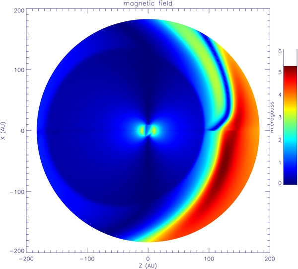
Figure 1. Magnetic field data used in our cosmic-ray modulation study.
Download figure:
Standard image High-resolution image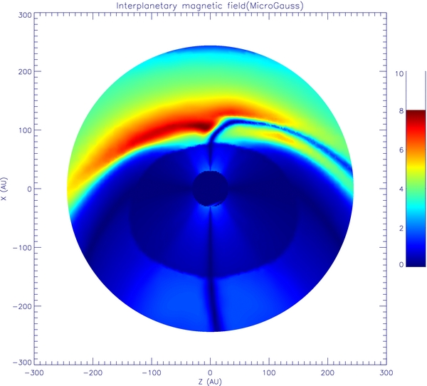
Figure 2. Magnetic field profile from Linde's MHD data set (Linde et al. 1998).
Download figure:
Standard image High-resolution image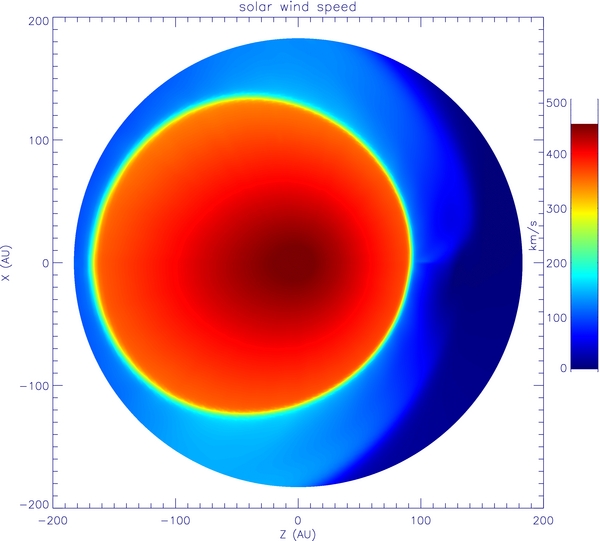
Figure 3. Solar wind speed used in our cosmic-ray modulation study.
Download figure:
Standard image High-resolution image
Figure 4. Solar wind speed from Linde's MHD data set (Linde et al. 1998).
Download figure:
Standard image High-resolution imageTable 1 illustrates the location of the TS in these MHD models along four different locations. It can be seen that the TS in the ecliptic plane is largely expanded in our MHD model compared with the model of Linde et al. (1998). The upwind location was moved from 70 AU to 91 AU, being more consistent with the crossing location of Voyager 1 (Stone et al. 2005) and the recent estimation made by Luo et al. (2011). Compared with the expansion in the ecliptic plane, the size of the TS in the polar direction has been reduced, which is due to the symmetrized effect caused by interstellar neutrals (Pogorelov et al. 2007). In the subsequent section, we will show that these changes affect the Galactic cosmic-ray modulation as well.
Table 1. The Location of the TS Toward Different Directions
| Direction | Linde's Model | Pogorelov's Model |
|---|---|---|
| (TS Distance AU) | (TS Distance AU) | |
| Upwind | 70 | 91 |
| Flank | 105 | 125 |
| Polar | 140 | 129 |
| Downwind | 150 | 169 |
Download table as: ASCIITypeset image
Both Figures 3 and 4 demonstrate that the TS is a closed boundary where the solar wind speed decreases from 400 km s−1 to nearly 130 km s−1. Inside the TS is the supersonic solar wind region where the solar wind speed is nearly symmetric.
As for the magnetic field profile, a difference between these two sets of MHD data also exists. The dark blue color denotes a vanishing magnetic field. Near the nose of the TS, a blue belt turns upward toward the northern area in our MHD data. This is the ISM-induced bending of the heliospheric current sheet, which is assumed to be flat in the supersonic SW ahead of the TS. The magnetic field will be mainly used to calculate cosmic-ray drift speed. The drift speed is very large near the current sheet because of the sudden reverse of the magnetic field direction. This is consistent with the well-known concept that cosmic rays experience very large drift speed along current sheets (Burger & Potgieter 1989).
Figure 5 provides a more straightforward demonstration of how the magnetic field varies with radial distance in the heliosphere. It shows the linear distribution of the magnetic field magnitude along three directions: the upwind direction, the Voyager 1 trajectory at 35°N heliolatitude, and the Voyager 2 trajectory at 35°S heliolatitude. It can be seen from this plot that the magnitude along these three directions decreases consistently inside the supersonic solar wind region. After the TS crossing, the magnitude of the magnetic field increases due to shock compression. However, for the upwind direction, after a short increase of the magnitude, the magnetic field experiences a sudden decrease. This is caused by the crossing of the current sheet. This crossing of the current sheet can also be seen in the Voyager 1 direction. Similar to the current sheet, another structure called the magnetic wall can also be seen in these curves. At around 150–200 AU, all three directions experience a peak in magnetic field, which we call the "magnetic wall." According to our simulation shown later, this strong magnetic field acts as a barrier that can reduce cosmic rays coming in from the ISM.
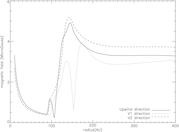
Figure 5. Linear distributions of the magnetic field magnitude along the upwind direction (solid line), Voyager 1 direction (dotted line), and Voyager 2 direction (dashed line).
Download figure:
Standard image High-resolution image2.2. Incorporating the MHD Data into the Galactic Cosmic-ray Modulation Model
While three-dimensional Galactic cosmic-ray transport simulation code has been developed by several groups (Kota & Jokipii 1983; Potgieter & Burger 1990), our code possesses a unique technique that has many advantages when dealing with an MHD heliosphere model. Instead of solving the Parker equation directly with the finite difference method, we solve for the stochastic phase space trajectory of a particle as a function of backward time s. This process begins from the location where we need to know the cosmic-ray flux (Zhang 1999) until it hits the boundary of the entire simulation domain, which is the outer boundary of the LISM. The solution to the Parker transport equation is the expectation value of all boundary values when the particle exits from the boundaries. The stochastic differential equation for the random particle trajectory corresponding to the Parker transport equation can be written as (Zhang 1999)


During each iterating step, the location and momentum of the pseudo-particle described by the stochastic differential equation will be updated. Here, dW is a three-dimensional random Wiener differential noise term, which can be generated using a Gaussian distribution random number with a mean of zero and a standard deviation of ds.  is the diffusion tensor, and it has the following form if expressed in the local magnetic field coordinates:
In our simulation, the diffusion tensor can be transferred to our spherical coordinates using the following form:
where ψ is the angle between the local magnetic field direction B and the radial direction r. Transformations to other coordinate systems can be done in a similar manner.
For the diffusion coefficient, we choose the following general form:
where p and B are the particle momentum and magnetic field strength, respectively, and β is the ratio of particle speed to the speed of light. The p0 parameter is a reference momentum (in our case 1 GeV c−1), Beq is the IMF strength at the heliospheric equator at 1 AU. The constants κ∥0 and κ⊥0 determine the magnitudes of parallel and perpendicular diffusion coefficients. They are chosen to be 50 × 1020 cm2 s−1 and 5 × 1020 cm2 s−1, respectively. The exponents are chosen as a∥, ⊥ = 0.5 and b∥, ⊥ = 1. The choice of the above diffusion coefficients is a little arbitrary, but it is approximately consistent with the overall modulation level inferred by various observations and a few other simulations of cosmic-ray modulation.
As for the drift velocity, we use the classical form (Jokipii et al. 1981)
Both the diffusion coefficient and drift velocity are functions of magnetic field and plasma speed. Thus, following Equation (5), it is essential to know the magnetic field and solar wind speed in order to calculate the location and momentum increments. This is done through direct numerical differentiation of the magnetic field vector on the MHD grids. When cosmic rays transport to any random location inside the heliosphere, a function for calculating the local diffusion coefficient and drift velocity is called into the stochastic differential equation (5).
2.3. MHD Data Interpolation and Curl and Divergence Calculation
In order to obtain the magnetic field and solar wind speed at any arbitrary point (r, θ, ϕ) inside the simulation domain, the discrete MHD data need to be interpolated. The original MHD data are based on a three-dimensional spherical coordinate system. According to the mesh grid system (Equation (4)), the simulation globe is divided into 220 spherical planes and on each plane, the angle difference between the two neighboring points is 2π/79 along azimuthal direction and π/140 along the latitudinal direction.
Thus, for any arbitrary point (r, θ, ϕ), there are eight adjoining grid points in the MHD data set: (ri, θi, ϕi), (ri, θi + 1, ϕi + 1), (ri, θi + 1, ϕi), (ri, θi, θi + 1) on the spherical plane with a radius of ri and (ri + 1, θi, ϕi), (ri + 1, θi + 1, ϕi), (ri + 1, θi, ϕi + 1), (ri + 1, θi + 1, ϕi + 1) on the spherical plane with a radius of ri + 1. In addition, the following relationship exists for these quantities, ri ⩽ r ⩽ ri + 1, θi ⩽ θ ⩽ θi + 1, ϕi ⩽ ϕ ⩽ ϕi + 1.
Using the value of these eight points, our interpolation method is achieved in two steps: (1) use the bilinear interpolation method (Press et al. 1992) to obtain the values at points (ri − 1, θ, ϕ) and (ri, θ, ϕ) separately and (2) after obtaining the values at these two projecting points, employ a linear interpolation method (Press et al. 1992) to obtain the local value at point (r, θ, ϕ). In this way the value at any arbitrary point inside the heliosphere can be obtained.
In order to obtain the drift speed, we need a numerical method to calculate the curl of a vector field. In this study, following definition of the curl in the spherical coordinate system, the finite difference method is used to calculate the gradient of each vector component (Press et al. 1992). Figure 6 shows a comparison made between our numerical result and the analytical result of the drift speed using Parker's magnetic field (Jokipii et al. 1977). Our numerical method is consistent with the analytical result. As for the current sheet drift, cosmic-ray particles will experience a very large drift velocity because of the sudden change in the direction of the magnetic field. An analytical calculation of the drift speed using a sharply reversed magnetic field across the current sheet yields a δ-function. A more accurate simulation of particle drift using realistic particle speed and trajectory still yields a peak drift speed of one-sixth of the particle speed at the center of the current sheet (Burger & Potgieter 1989) and an enhanced drift speed appears within a four particle gyroradius from the current sheet. In our numerical calculation, the drift speed is not that large but the profile of the enhanced current sheet drift is much thicker because of a limited resolution of our MHD grid. It turns out that as long as the magnitude of the current sheet drift times the thickness is conserved, the effect of current sheet drift on cosmic-ray modulation remains the same. An advantage of this thickened current sheet drift is that we can still use a relatively large integration step size of ∼0.1 AU and do not miss the chance to see a possible large current sheet drift as cosmic-ray particles approach the current sheet. With the help of our 512 node high-performance computer, the numerical integration is still stable even with these large current sheet drift velocities. Thus, the classical form of drift velocity with a straightforward numerical calculation of the current sheet drift is still utilized.

Figure 6. Drift speed along a specific direction using Parker's magnetic field. The line is from the analytical form by Jokipii et al. (1977). The diamond shows the results using our numerical method.
Download figure:
Standard image High-resolution imageHowever, we encounter difficulty with a finite MHD grid resolution in the calculation of DSA using the TS. The grid size of our MHD model is roughly 1 AU at the radial distance of the TS. With numerical dissipation, the TS looks unrealistically wide at about 4 AU. In contrast, the observed thickness of the TS is only a few hundred thousand km (Richardson et al. 2008). As pointed out by Zhang (2007), the ratio of the diffusion coefficient to the product of the upstream plasma speed and the shock thickness affect the resulting accelerated particle spectrum. Only when this ratio is significantly above 1 can the DSA results be approached. With a shock ramp 4 AU thick, the ratio for most cosmic-ray particles falls below 1 and the effect of DSA is underestimated. In order to avoid any possible effect from a smoothed shock, in this study we use a hyperbolic function to sharpen the TS. Following Equation (9), the solar wind speed profile can be sharpened,

where rts is the location of the TS and Vup and Vdown are the solar wind speed upstream and downstream of the TS, respectively. The coefficient w determines the width of the TS. If we choose w = 0.1, it produces a shock profile with a ramp width of ∼0.2 AU thick. Figure 7 shows the sharpened TS and original MHD shock profile. Similarly, the magnetic field profile near the shock is also sharpened.

Figure 7. Simulated radial flux pointing toward the 55°N nose direction for different cosmic-ray energy levels.
Download figure:
Standard image High-resolution image3. RESULTS
With the cosmic-ray modulation code, we set out to run a number of simulations. The outer boundary of our simulation is set to be 200 AU, which is large enough to include both the inner and outer heliosheath. The following form for the local interstellar spectrum (LIS) is chosen:

The radial distance of the outer boundary is slightly arbitrary, but it should be large enough compared to the location at which the modulated cosmic-ray fluxes are calculated. We chose 200 AU because it is significantly beyond the heliopause and we are mainly concerned with the cosmic-ray flux in the inner heliosheath or closer regions. The shape of the LIS is chosen to roughly match our calculation results to some observed spectra.
In the following, the radial flux (differential flux along radial direction ( ) in the simulation domain) for different MHD heliosphere data sets, and different energy levels in the heliosphere will be discussed. The energy spectrum will also be given and compared with the measurements from the Voyager 1 mission. We will show how cosmic-ray transport behaves in the new global MHD heliosphere.
3.1. Radial Profiles of Cosmic-ray Flux
Figure 7 shows some radial profiles of cosmic-ray flux for a number of different energy levels (1 GeV, 800 MeV, 600 MeV, 400 MeV, 300 MeV, 200 MeV) in the direction pointing to 55°N heliolatitude and 0° heliolongitude. Figure 8 shows the flux along the upwind direction, or exactly to the nose of the heliosphere, for a number of energy levels (1 GeV, 800 MeV, 600 MeV, 300 MeV, 200 MeV). The TS has been sharpened to less than 0.2 AU so that the DSA is not underestimated. In general, our simulations illustrate the basic trend of the cosmic-ray radial flux. It increases from the inner heliospheric region to the ISM until it reaches its corresponding LIS flux value. Both the heliosheath and the TS contribute to the modulation. (There will be a detailed discussion about the effect of DSA caused by the TS in the next section.) Both Figures 7 and 8 show that the heliosheath region contributes to the modulation. Thus, the LIS can only be obtained after the Voyager spacecraft (or future spacecraft) fully enter into the LISM.
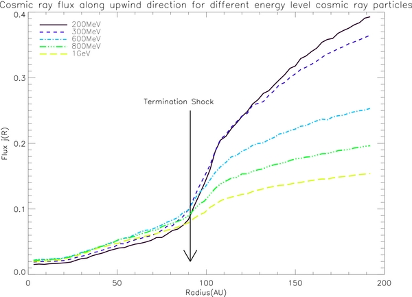
Figure 8. Simulated radial flux along the upwind direction for different cosmic-ray energy levels.
Download figure:
Standard image High-resolution imageBased on these two simulations, we can calculate the radial gradient of cosmic-ray flux given by the following formula:
In the supersonic solar wind region, the radial gradients for 200 MeV, 300 MeV, and 600 MeV along the upwind direction are 2.03% (AU−1), 2.01% (AU−1), and 1.83% (AU−1), respectively. Using Ulysses data, Heber et al. (2002) estimated that for protons with energy greater than 250 MeV, the radial gradient was 2.2% ± 0.6% (AU−1) before early 1998 and 3.5% (AU−1) thereafter. Our simulation result agrees with the value before early 1998, a solar minimum year. As previously stated, this is because the MHD data we have used have a flat current sheet, representing the solar minimum condition in a positive polarity period.
The radial gradients change after the TS in the local direction. These gradients are much larger than the values in the supersonic solar wind region before becoming smaller in the heliosheath (∼50 AU in Figure 7 and ∼20 AU in Figure 8 downstream of the TS crossing). These large radial gradients occur in transition regions where magnetic field lines can intersect the TS at different longitudes. In some manner, the effect of a non-spherical shock appears to contribute quite a bit to the cosmic-ray radial gradient in this region around the TS. Once deep in the heliosheath, the radial gradients settle down to their own levels according to particle energy. At high energies, the radial gradients can become smaller than in the supersonic solar wind.
In comparison, Figure 9 shows the radial flux of 600 MeV protons along the upwind direction using two sets of MHD data (one from Linde and the other from Pogorelov). Although we use the same form of LIS and diffusion coefficients, these two sets of MHD data give different radial profiles of cosmic-ray flux. Specifically, the Galactic cosmic-ray flux inside the TS decreases significantly using the new MHD data from Pogorelov et al. (2008) with a more correct treatment of interstellar neutral atoms. Our new results here are more in line with the simulation by Florinski & Pogorelov (2009), but there are still some differences.
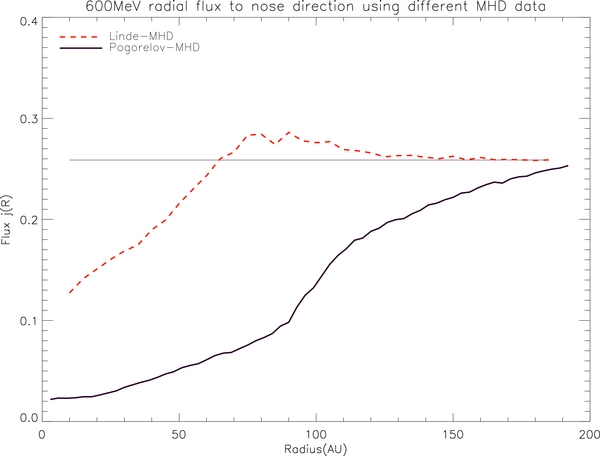
Figure 9. Simulated radial flux along the upwind direction using two different sets of MHD data.
Download figure:
Standard image High-resolution imageAfter considering the momentum and energy transfer between these interstellar neutral atoms and solar wind protons, the region inside the TS expands significantly (see Table 1). The increased cosmic-ray modulation level probably comes from the geometric extension of the TS. Cosmic-ray particles encounter the supersonic solar wind in a much larger region. Due to the convective effect, solar wind expels the incoming stream of cosmic-ray particles. In accordance with this, the modulation level increases and the cosmic-ray intensity decreases. Another factor that can affect cosmic-ray modulation is the shape of the TS. The TS became less asymmetric in our new MHD model which treats interstellar neutrals. A previous study by Caballero-Lopez et al. (2004) also found that the shape of the TS affects cosmic-ray transport.
3.2. The Effect of Diffusive Shock Acceleration Caused by TS
In comparison with the work done by Florinski & Pogorelov (2009), our simulated radial profiles of cosmic-ray flux begin to show an increase in radial gradient roughly at the location of the TS. This is consistent with the previous scenario. Cosmic-ray particles gain energy by crossing the TS because of the DSA. Since the cosmic-ray intensity in the lower energy region of the LIS is higher, the cosmic-ray intensity value around the TS region will show a jump in radial gradient (Kota & Jokipii 1983).
To illustrate the effect of the TS and to explain our results more clearly, we simulate cosmic-ray transport in a heliosphere with a spherical TS so that the effect is concentrated at one radial distance. Figure 10 shows how the TS affects the radial flux using our previous analytical cosmic-ray modulation code, which adapts the standard Parker's IMF model (Zhang 1999). The shock is treated as a step function, where the solar wind speed suddenly decreases. The skew Brownian motion method proposed by Zhang (2000) was also used to calculate DSA. Clearly, after the acceleration effect of the TS is removed, the radial flux decreased. The largest flux decrease happens at the TS location, and the apparent radial gradient change is seen at the TS. In addition, since a spherical shock with a radius of 92 AU is used, the change in the cosmic-ray flux gradient is exactly located at 92 AU. These results strongly support the fact that DSA affects cosmic-ray transport inside the heliosphere and the flux value around the shock increases as a result of acceleration.
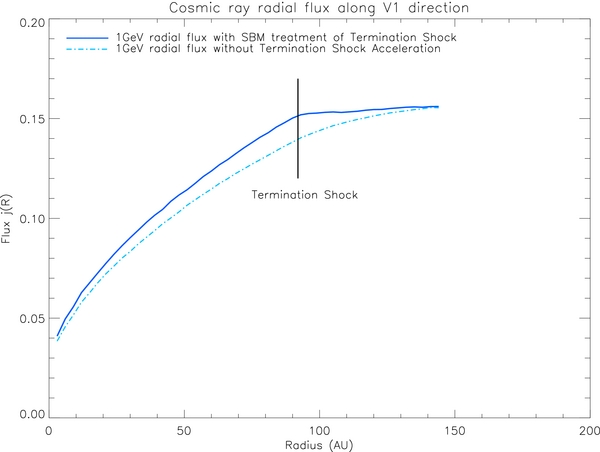
Figure 10. Simulated radial flux for 1 GeV cosmic rays. The skew Brownian motion (SBM) method (Zhang 2000) was used to treat the DSA caused by the TS.
Download figure:
Standard image High-resolution imageIn our current MHD heliospheric model, the shock is not an abrupt boundary. The hyperbolic function tanh is used to sharpen the TS (Equation (9)). The shock width can also be changed to see how it affects the radial flux. Figure 11 shows how the radial flux for 300 MeV cosmic-ray particles varies as shocks with different widths are used. (In order to highlight the difference of the radial flux caused by different treatment of the TS, the log scale is used in this plot. In addition, since the interstellar intensity for 300 MeV cosmic-ray particles is relatively higher, Figure 11 looks different from Figure 10.) It has been shown that the skew Brownian motion method gives the largest flux value since the shock is treated as a step function and the width of the TS is infinitely thin. When the width of the TS increases from 0.2 AU to 2 AU, the flux value also decreases. The cosmic-ray intensity level is the lowest for the case without acceleration by the TS.

Figure 11. Simulated radial flux for 300 MeV cosmic rays. The flux value varies due to the use of a different method to treat the DSA caused by TS.
Download figure:
Standard image High-resolution imagePreviously, Jokipii et al. (1993) and Caballero-Lopez et al. (2004) also investigated the TS effect on cosmic-ray modulation. They saw change in radial gradient across the TS. Their methods of calculation are different from ours, but we reach the same conclusion.
While the change in the radial flux gradient (Figure 10) appears at just one location using the analytical spherical shock model, the flux curve (Figures 7 and 8) obtained from the cosmic-ray transport code using the MHD plasma background shows a wide transition region at the TS. This is probably due to the asymmetric shape of the TS in the MHD data. Since the location of the TS varies on different field lines, the effect of shock acceleration can propagate to some distance away.
3.3. Latitude and Longitude Dependence of the Radial Flux Profile
As pointed out by Jokipii et al. (1979), the drift effect causes the latitude difference in the radial flux. During the solar minimum period, when the polarity of the Sun's magnetic field is positive, most cosmic-ray particles enter inward from the heliospheric polar region and outward near the ecliptic plane region. The intensity of the cosmic-ray particles in the ecliptic plane is lower than in the polar region. The overall latitudinal gradient is positive. Our simulation result has confirmed this scenario. Figure 12 shows the simulated cosmic-ray radial flux for different latitudes toward the nose direction. In the inner heliosphere, the flux increases as the heliolatitude increases. However, the situation reverses in the heliosheath. The flux in the lower heliolatitude is higher. This is probably attributed to the fact that diffusion is more important than drift inside the heliosheath. Another factor that can cause this result is the northward flip of the current sheet (see Figure 1). As the current sheet flips northward, most of our simulated time-backward particles exit the outer boundary near the polar region.
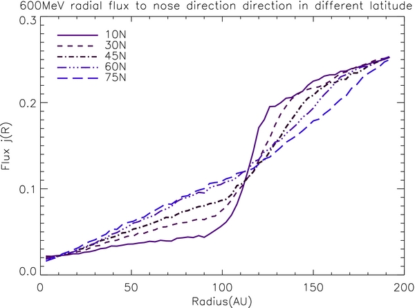
Figure 12. Simulated radial flux for 600 MeV cosmic rays along different latitudes in the northern heliosphere pointing toward the heliospheric nose.
Download figure:
Standard image High-resolution imageThe radial flux in the southern heliosphere also changes with latitude. Figure 13 shows how the radial flux varies with latitude in the southern heliosphere. The simulation shows nearly the same trend as in the northern heliosphere. In the inner heliosphere, the radial flux increases as the latitude increases, and the latitudinal gradient is positive. The situation reverses in the outer heliosphere, where the flux near the ecliptic plane region has a higher value.
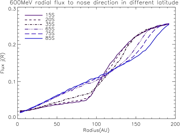
Figure 13. Simulated radial flux for 600 MeV cosmic rays along different latitudes in the southern heliosphere pointing toward the heliospheric nose.
Download figure:
Standard image High-resolution imageFigure 14 shows a comparison between our calculated cosmic-ray energy spectra at several locations. At the same radial distance (either 105 AU or 65 AU), the spectra at 55°S and 55°N are almost identical, but the spectra at the flank (90° from the nose in the longitudinal direction) are significantly different from those at the nose. This tells us that the variation of cosmic-ray flux strongly depends on longitude. This conclusion was not obtained by previous studies with a two-dimensional symmetric model because the longitude effect was neglected (Haasbroek & Potgieter 1998).

Figure 14. Simulated energy spectra at 105 AU and 65 AU with different longitudes. 105AU-55N-0, 105AU-55S-0, 65AU-55N-0, and 65AU-55S-0 represent the same points as in Figure 16, e.g., (105 AU, 55°N, 0° nose); (105 AU, 55°S, 0° nose); (65 AU, 55°S, 0° nose); and (65 AU, 55°N, 0° nose). The blue dash-dotted line labeled 105AU-55N-90 represents the solution at (105 AU, 55°N, 90° flank), and the green dash-dotted line labeled 65AU-55N-270 represents the solution at (105 AU, 55°N, 270° flank).
Download figure:
Standard image High-resolution imageThe actual longitude gradient varies with a particle's energy level. Table 2 shows the longitude gradient (the percentage of cosmic-ray flux difference per degree from the nose to flank) for a number of energies. All these gradient values are calculated based on the simulation result shown in Figure 14.
Table 2. Flux Values for Different Energy Levels at 105 AU N and (105 AU, 90°, 35°) and Associated Longitude Gradient
| Energy | (105 AU, 55°, 0°) Flux | (105 AU, 55°, 90°) Flux | Longitude Gradient  |
|---|---|---|---|
| (GeV) | |||
| 0.2 | 0.08837 | 0.13557 | 0.47% |
| 0.25 | 0.08709 | 0.13804 | 0.50% |
| 0.3 | 0.08196 | 0.13757 | 0.56% |
| 0.35 | 0.07910 | 0.13803 | 0.60% |
| 0.4 | 0.07714 | 0.13748 | 0.62% |
| 0.45 | 0.07192 | 0.13258 | 0.66% |
Note. 105 AU N = (105 AU, 55°, 0° nose); (105 AU, 90°, 35°) = (105 AU, 55°, 90° flank).
Download table as: ASCIITypeset image
3.4. North–South Asymmetry of Cosmic-ray Flux
Since a global asymmetry exists in the north–south dimensions of the heliosphere, cosmic-ray transport behaves differently in these two hemispheres. Figure 15 illustrates how the north–south asymmetry affects the radial flux. Although the asymmetric effect exists both inside and outside the TS, it varies with latitude. Near the ecliptic plane (10°), the radial flux in these two hemispheres is nearly the same for r < 90 AU or inside the TS. The flux varies as the latitude increases. Up to 60°, the flux difference along the same latitude in the northern and southern heliosphere already becomes significant, even inside the TS.
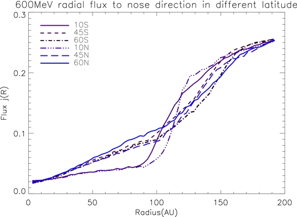
Figure 15. Simulated radial flux for 600 MeV cosmic rays along different latitudes pointing toward the nose direction. The radial flux in the northern and southern heliospheres is shown together for comparison.
Download figure:
Standard image High-resolution imageThis north–south asymmetrical effect has also been explored by Ngobeni & Potgieter (2011). They compared the radial flux along the Voyager latitudes of 35°N and 35°S and found that for E > 200 MeV cosmic rays, the effect of north–south asymmetry is insignificant.
Figure 16 shows the simulated energy spectra at (105 AU, 55°N, 0° nose longitude) and (65 AU, 55°N, 0° nose longitude) in the northern heliosphere. For comparison, the energy spectra in the southern heliosphere, i.e., the energy spectra at locations (105 AU, 55°S, 0° nose longitude) and (65 AU, 55°S, 0° nose longitude) are also shown. This demonstrates that in the region inside the TS, there is little difference between the spectra at the northern and southern heliosphere. As the simulation location is moved outward of the TS, these spectra show greater difference, particularly in the lower energy end. The north–south asymmetry of the heliosphere seems to have a more significant effect on lower energy cosmic-ray particle transport.
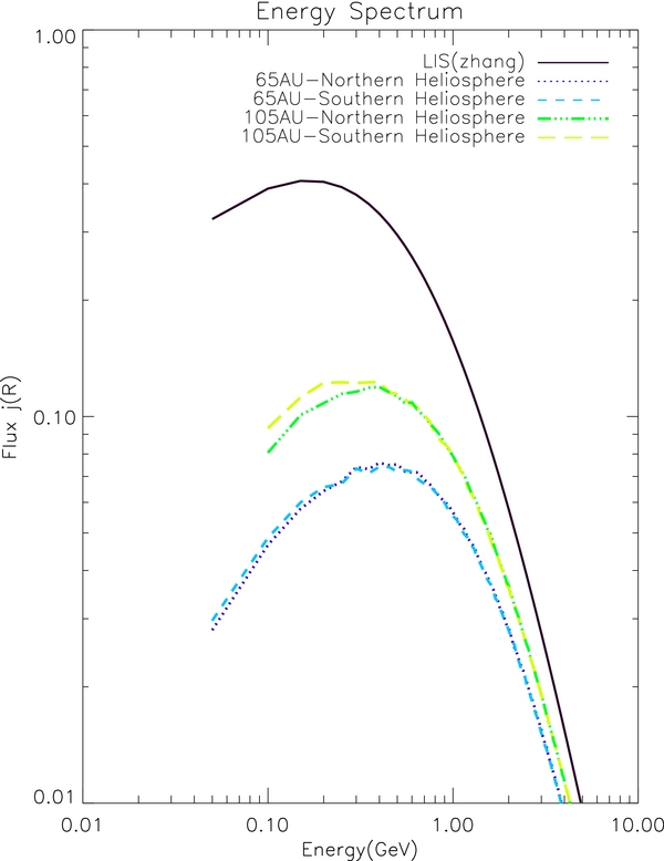
Figure 16. Simulated energy spectra at radial distances of 65 AU and 105 AU. The green dash-dotted line represents the solution at (105 AU, 55°N, 0° nose) and the yellow dashed line represents the solution at (105 AU, 55°S, 0° nose). For the 65 AU case, the blue dashed line represents the spectra at (65 AU, 55°S, 0° nose) and the purple dotted line represents the spectra at (65 AU, 55°N, 0° nose).
Download figure:
Standard image High-resolution image3.5. The Effect of the LIS
Since the shape of the LIS specifies the boundary condition in the numerical simulation, the cosmic-ray intensity value inside the heliosphere depends on the choice of input for the LIS. As of now, there is still no direct observational approach for obtaining the LIS. Only by using a diffusion model for cosmic-ray propagation in the Galaxy can the LIS form be indirectly calculated (Webber & Higbie 2009). In the following paragraphs, simulated energy spectra using different LIS forms will be shown to illustrate the LIS effects on cosmic-ray modulation.
Figure 17 demonstrates the energy spectra at 105 AU in the northern heliosphere 55° N and southern heliosphere 55° S using different LIS forms. One is from Equation (10), and the other is from the recent result of LIS obtained by Webber & Higbie (2009), which can be fitted by the following function:
The simulation result shows that using a new LIS form does not change the previous results, once we normalized Zhang's LIS to the LIS of Webber & Higbie (2009) at the high-energy end. North–south asymmetry still does not show up at the higher energy end for the simulated spectrum plot; the flux in the southern heliosphere is slightly larger than the flux in the northern heliosphere only for the E < 300 MeV cosmic rays.

Figure 17. Simulated spectra at (105 AU, 55°N, 0° nose) and (105 AU, 55°S, 0° nose) using different sets of LIS forms. The green dash-dotted curve labeled "105 AU (Webber)-N" illustrates the spectrum solution at (105 AU, 55°N, 0° nose), using Webber's LIS, while the curve labeled "105 AU (Webber)-S" illustrates the spectrum solution at (105 AU, 55°S, 0° nose) in the southern heliosphere. Similar notation applies to the other two spectrum curves.
Download figure:
Standard image High-resolution imageSimilarly, Figure 18 shows the energy spectra at 65 AU in the northern and southern heliosphere using different LIS forms. Regardless of whether Zhang's or Webber's LIS is used, the north–south asymmetry effect is small.
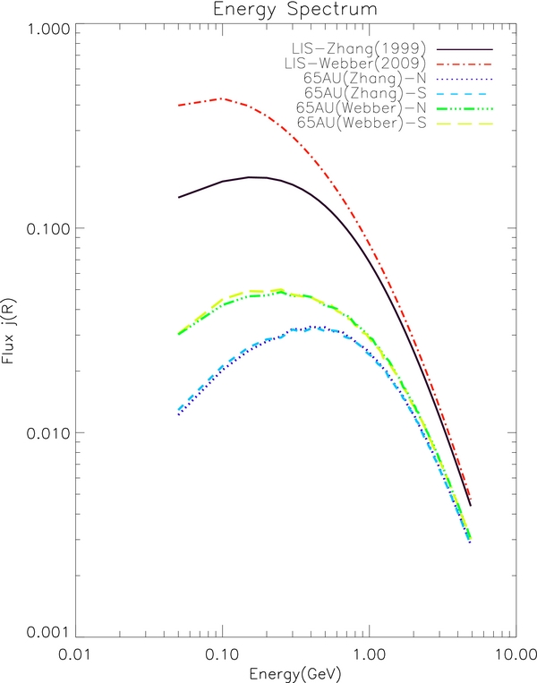
Figure 18. Simulated spectra at (65 AU, 55°N, 0° nose) and (65 AU, 55°S, 0° nose) using different sets of LIS forms. The purple dotted curve labeled "65 AU (Zhang)-N" represents the spectrum solution at (65 AU, 55°N, 0° nose) in the northern heliosphere using Zhang's LIS, while the blue dashed curve labeled "65 AU (Zhang)-S" illustrates the spectrum at (65 AU, 55°S, 0° nose) in the southern heliosphere.
Download figure:
Standard image High-resolution imageFigure 19 shows the radial flux along the upwind direction using these two sets of LIS. Once the fluxes are normalized, the two curves are almost the same. For example, considering the case using the LIS from Webber, the flux level at 90 AU is 0.0576. Comparing this value to the LIS value 0.1526, the whole heliosheath and TS region contribute (0.1526 − 0.0576)/0.1526 ≈ 62.3% to the global modulation. On the other hand, using Zhang's LIS (Equation (10)), the LIS value is 0.2575, and the flux at 90 AU is 0.0982. The modulation outside the TS is (0.2575–0.0982)/0.2575 ≈ 61.9%, which is nearly the same as the previous value. Therefore, regardless of LIS form, the relative contribution from different regions is the same. In addition, the radial gradient inside the TS using the Webber–Higbie LIS is 1.87% AU−1, which is similar to the radial gradient value 1.83% AU−1 using Zhang's LIS.
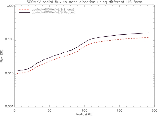
Figure 19. Simulated radial flux for 600 MeV cosmic rays along the upwind direction using different sets of LIS forms.
Download figure:
Standard image High-resolution image3.6. Simulation of Cosmic-ray Flux along Voyager Directions
Since our cosmic-ray transport model is three-dimensional, a realistic simulation of the radial flux along the Voyager spacecraft's direction can be made. In our simulation, the direction of Voyager 1 is assumed along (35°N, 0° (nose)), and Voyager 2 along (30°S, 40° (nose)). Although the latitude varies along Voyager 1 and 2's real trajectories, the simulation shows that the latitude variation does not affect the simulated radial flux. Figure 20 illustrates the radial flux comparison between the real Voyager 2 trajectory and the simplified trajectory without the latitude change. Within a 5% difference, these two flux curves are nearly the same. This difference does not affect our qualitative study.
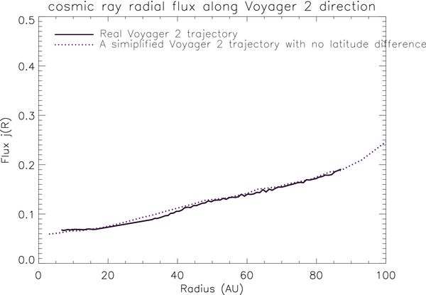
Figure 20. Simulated cosmic-ray radial flux between the real Voyager 2 trajectory (from http://cohoweb.gsfc.nasa.gov/helios/heli.html) and a simplified Voyager 2 trajectory, without the latitude change.
Download figure:
Standard image High-resolution imageFigure 21 shows the radial profiles of cosmic-ray flux along the Voyager 1 and Voyager 2 directions. It demonstrates obviously different radial fluxes. Because the latitude variation does not significantly affect the result, this implies that the longitudinal difference causes the radial gradient difference in the Voyager 1 and Voyager 2 directions. However, with previous two-dimensional simulations for Voyager 1 and 2, the longitudinal difference in cosmic-ray radial flux may be easily neglected (Manuel et al. 2011).

Figure 21. Simulated cosmic-ray radial flux along the Voyager 1 and 2 trajectories.
Download figure:
Standard image High-resolution imageIf we assume the speeds of the Voyager spacecraft are constant, the radius and time relationship for Voyager 1 and 2 can be derived as
Then we can predict the cosmic-ray fluxes along Voyager 1 and 2's directions as a function of time (Figure 22). The prediction shows that Voyager 1's flux is higher than Voyager 2's before 2012, which agrees with observations, since the cosmic-ray subsystem (CRS) measurement value for Voyager 2 never exceeds that of Voyager 1. However, the apparent radial gradient derived from a direct comparison of the cosmic-ray flux at Voyager 1 and Voyager 2 tends to underestimate the true radial gradient. For example, in 2012 January, Voyager 1 was about 120 AU far from the Sun, while Voyager 2 was 20 AU behind, about 98 AU from the Sun. The simulated 180 MeV cosmic-ray flux at 120 AU (Voyager 1's location) is 0.237 and 0.234 at 98 AU (Voyager 2's location). Thus, the apparent radial gradient nearly vanishes (0.01% per AU) if one uses the two Voyagers' cosmic-ray flux difference. However, based on the simulation result, the radial gradient along Voyager 1 is about 0.2% AU−1 at 120 AU and about 0.3% AU−1 along Voyager 2 at 98 AU (nearly 30 times larger than the apparent radial gradient). This demonstrates how longitude affects the cosmic-ray radial profile. After 2012, the flux values for the two spacecraft will become comparable, even though there is still a radial gradient in Figure 21. At some point, Voyager 2 may even see a higher cosmic-ray flux than Voyager 1, but this does not mean that the true radial gradient of the cosmic-ray flux is negative.

Figure 22. Prediction for the cosmic-ray intensity measured by Voyager 1 and 2's CRS.
Download figure:
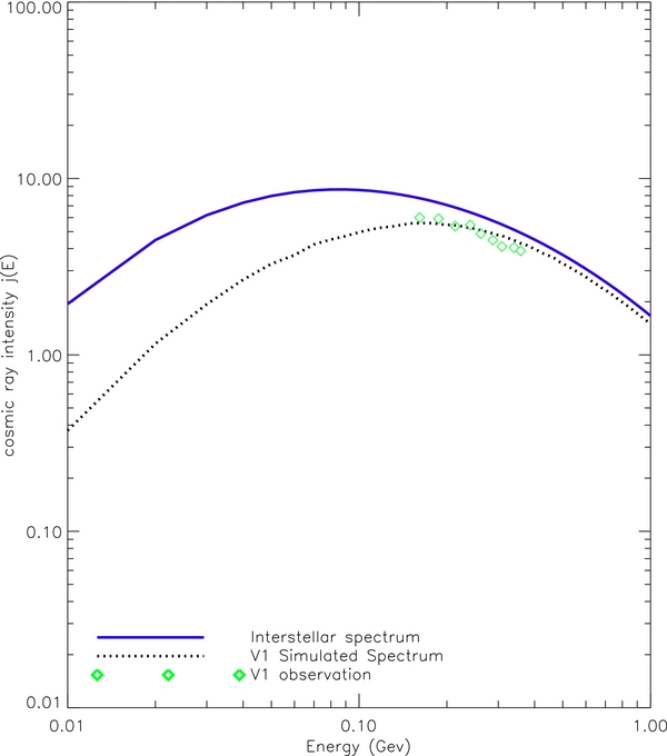
Standard image High-resolution imageFigure 23 shows the simulated proton spectrum at 2008 Voyager 1's location. The cosmic-ray measurement from Voyager 1 (Webber et al. 2008) is also shown in the same plot. In this simulation, the LIS used is from Webber & Higbie (2009). It can be seen from the plot that our simulated spectrum is roughly within the measured spectrum of the proton.
Figure 23. Simulated cosmic ray at the 2008 Voyager 1 location compared with its observation. Intensities j(E) are in particles/m2 sr s MeV/nuc.
Download figure:
Standard image High-resolution image
4. SUMMARY
In this paper, we incorporated a realistic MHD heliospheric model into a cosmic-ray modulation code. Compared with our previous MHD model, the TS becomes significantly expanded and more symmetric because of the effect of the interstellar neutral atoms. These changes cause the cosmic-ray modulation level to increase. In addition, with the effect of DSA caused by the TS, the radial profile of cosmic-ray flux shows a change of radial gradient approximately in the TS region, resulting in a difference in the radial gradient of cosmic-ray flux across the TS. The change of radial gradient does not occur exactly at the TS radial distance in the same direction, indicating that the acceleration effect comes from a part of the TS at other longitudes or latitudes. The shock acceleration effect can be easily lost if the TS is unrealistically smoothed due to a lack of spatial resolution in previous MHD simulations.
Based on the simulated radial profiles of cosmic-ray flux, a latitude effect was also found. Inside the TS, the radial flux shows a positive latitude gradient and outside the TS, it shows a negative latitude gradient. Using our cosmic-ray modulation code, effects of north–south asymmetry, longitude, and different LIS forms were also illustrated.
In addition, since the heliospheric MHD data are three-dimensional, the radial profiles of cosmic-ray flux along the Voyager 1 and 2 trajectories can be simulated. It was found that the radial gradients significantly differ along these two directions, and this difference is mainly from the longitudinal effect. The apparent near-zero radial gradient of cosmic-ray flux derived directly from the data from the two Voyager spacecraft does not reflect the true radial gradient in either of the directions because of the longitudinal effect. Therefore, the measured radial gradient cannot be used to extrapolate the level of cosmic-ray flux in the local interstellar space.
Finally, the cosmic-ray energy spectrum is also compared with the spectrum observed by Voyager 1. The simulated spectrum agrees very well with the observed one, which indicates our hypothesis about the LIS is not too far from the real one.
This work was supported in part by NASA grants NNX08AP91G, NNX09AG29G, and NNX09AB24G. All simulation work was performed on the FIT Blueshark Cluster, which is supported by the National Science Foundation under grant No. CNS 09-23050. We thank the National Space Science Data Center for providing the Voyager Interplanetary Cruise Trajectory Data.