


ABSTRACT
By analyzing the X-ray spectra of NGC 3516 from 2001 and 2006 obtained with the HETGS spectrometer on board the Chandra X-ray Observatory, we find that the kinematic structure of the outflow can be well represented by four outflow components intrinsic to NGC 3516: −350 ± 100 km s−1, −1500 ± 150 km s−1, −2600 ± 200 km s−1, and −4000 ± 400 km s−1. A local component at z = 0 could be confused in the spectrum with intrinsic component 3. Components 1 and 2 have a broad range of ionization manifested by absorption from 23 different charge states of Fe. Components 3 and 4 are more highly ionized and show absorption from only nine different charge states of Fe. However, we were able to reconstruct the absorption measure distribution for all four. The total column density of each component is NH = (1.8 ± 0.5) × 1022 cm−2, (2.5 ± 0.3) × 1022 cm−2, (6.9 ± 4.3) × 1022 cm−2, and (5.4 ± 1.2) × 1022 cm−2, respectively. The fast components 3 and 4 appear only in the high state of 2006 and not in 2001, while the slower components persist during both epochs. On the other hand, there is no significant absorption variability within days during 2001 or 2006. We find that the covering factor plays a minor role for the line absorption.
Export citation and abstract BibTeX RIS
1. INTRODUCTION
Approximately half of type 1 active galactic nuclei (AGNs) show complex absorption in the soft X-ray band (Crenshaw et al. 2003; Piconcelli et al. 2005). The blueshifted absorption lines come from a highly or partly ionized outflow first noted by Halpern (1984). These outflows may play a central role in cosmological feedback, in the metal enrichment of the intergalactic medium, and in understanding black hole evolution. However, the outflow physical properties such as mass, energy, and momentum are still largely unknown. A necessary step to advance on these issues is to obtain reliable measurements of the ionization distribution and column densities of the outflowing material as well as the location of these outflows in order to determine the mass outflow.
NGC 3516 is a Seyfert 1 galaxy at a redshift z = 0.008836 (Keel 1996). It exhibits a variable relativistic Fe Kα emission line (Nandra et al. 1997, 1999) which could consist of a few narrow components (Turner et al. 2002). UV observations of NGC 3516 showed several outflowing components. Kriss et al. (1996a) found a low velocity component of ∼−300 km s−1 while also observing lines at close to the systemic redshift velocity (−2649 km s−1). Crenshaw et al. (1999) revealed four slow components with outflowing velocities of −31, −88, −148, and −372 km s−1. Kraemer et al. (2002) later detected UV absorption up to velocities of −1300 km s−1.
There are many studies in the literature of the ionized X-ray absorber of NGC 3516, the most important of which are listed in Table 1. Not all reports on the outflow of NGC 3516 are consistent, as described below. Kolman et al. (1993) analyzed a Ginga observation from 1989 and found an absorber with a partial covering factor. Mathur et al. (1997) found a −500 km s−1 outflowing component using a ROSAT observation from 1992. Kriss et al. (1996b) fitted ASCA data from 1994 with two absorption components, both outflowing with <−120 km s−1. Reynolds (1997) fitted the 1995 ASCA data with a single component. Costantini et al. (2000) studied BeppoSAX data from 1996 and 1997 and fitted two ionization components outflowing at velocities of −500 km s−1. Netzer et al. (2002) fitted ASCA data from 1998 and Chandra LETG data from 2000 with a single component. Using 2001 partially simultaneous Chandra, BeppoSAX, and XMM-Newton observations, Turner et al. (2005) identified three components: the −200 km s−1 component was called the "UV absorber," the second was called "High" at −1100 km s−1, and the third that was called "Heavy" was also at −1100 km s−1, but coverage of the source varied, which explained changes in the continuum curvature. Markowitz et al. (2008), based on a Suzaku 2005 observation, found two components: one was fitted with an outflow velocity of −1100 km s−1, while the other was stationary. Turner et al. (2008) studied Chandra and XMM-Newton observations from 2006 and identified four components. Two components were static while the third ("heavy" which also had a partial covering factor) and fourth ("high") had higher outflow velocities of −1575 and −1000 km s−1, respectively. Recently, Mehdipour et al. (2010) analyzed an XMM-Newton observation of NGC 3516 from 2006 and identified three components outflowing at velocities of −100, −900, and −1500 km s−1. The fastest component also had a partial covering factor.
Table 1. Historical Observations of NGC 3516
| Observatory | Year | Duration | Flux Level at 1 keV | Referencesa |
|---|---|---|---|---|
| (10−3 photon cm−2 | ||||
| (ks) | s−1 keV−1) | |||
| Ginga | 1989 Oct | 20 | 6 ± 1 | 1 |
| ROSAT | 1992 Oct | 13 | 17 ± 3 | 2 |
| ASCA | 1994 Apr | 28 | b 13 ± 2 | 3 |
| ASCA | 1995 Mar | 33 | b 7 ± 1 | 4 |
| BeppoSAX | 1996 Nov | 16 | 1 ± 0.5 | 5 |
| BeppoSAX | 1997 Mar | 16 | 7 ± 2 | 5 |
| ASCA | 1998 Apr | 360 | b 3 ± 0.5 | 6 |
| Chandra | 2000 Oct | 47 | b 0.6 ± 0.2 | 6 |
| Chandra | 2001 Apr | 119 | 1.5 ± 0.2 | 7,11 |
| XMM-Newton | 2001 Apr | 49 | 1.7 ± 0.2 | 7 |
| Chandra | 2001 Nov | 88 | 0.9 ± 0.2 | 7,11 |
| XMM-Newton | 2001 Nov | 49 | 1 ± 0.2 | 7 |
| Suzaku | 2005 Oct | 135 | 0.6 ± 0.2 | 8 |
| Chandra | 2006 Oct | 200 | 5 ± 0.5 | 9,11 |
| XMM-Newton | 2006 Oct | 155 | 5 ± 0.5 | 9,10,11 |
Notes. a(1) Kolman et al. 1993; (2) Mathur et al. 1997; (3) Reynolds 1997; (4) Kriss et al. 1996b; (5) Costantini et al. 2000; (6) Netzer et al. 2002; (7) Turner et al. 2005; (8) Markowitz et al. 2008; (9) Turner et al. 2008; (10) Mehdipour et al. 2010; (11) present work. bNetzer et al. (2002) finding of long-term decline over years is fortuitous.
Download table as: ASCIITypeset image
In this paper, we wish to provide a definitive investigation of the physical conditions in the NGC 3516 X-ray absorber, using the archival HETGS observation from 2001 and 2006 and exploiting its high spectral resolution, but with special focus on the ionization distribution of the plasma and on lines that do not seem to fit the simple two-velocity picture. While the majority of studies on the X-ray spectra of AGN outflows employ gradually increasing numbers of ionization components until the fit is satisfactory (e.g., Kaspi et al. 2001; Sako et al. 2003), it is instructive to reconstruct the actual distribution of the column density in the plasma as a continuous function of ionization parameter ξ (Steenbrugge et al. 2005), which we termed the absorption measure distribution (AMD; Holczer et al. 2007). Although for high-quality spectra such as the present one, two or three ionization components might produce a satisfactory fit, the AMD reconstruction is the only method that reveals the actual distribution including its physical discontinuities (e.g., due to thermal instability), and ultimately provides a more precise measurement of the total column density. Furthermore, the AMD shape can impose tight constraints on physical outflow models and on the density distribution in the outflow (Chelouche 2008; Behar 2009; Fukumura et al. 2010, 2011).
2. DATA REDUCTION
NGC 3516 was observed by Chandra/HETGS on 2001 April 9–10 and November 11, as well as on 2006 October 9–14 for a total exposure time of 407 ks. In each observation, the first three high energy gratings (HEG) and medium energy gratings (MEG) refraction orders (±1, 2, 3) were reduced from the Chandra archive using the standard pipeline software (CIAO version 4.1.2). The total number of counts in the first order (±1) between 2 and 25 Å is 141,663 for MEG and 75,043 for HEG. More details on the observations can be found in Table 2. No background subtraction was required as the background level was negligible. Flux spectra were obtained by first co-adding count spectra and convoluting with the broadest line-spread function (MEG first order) to ensure uniformity. The total count spectra were then divided by the total effective area curve (summed over orders) and observation time. Finally, spectra were corrected for neutral Galactic absorption of NH = 3.23 × 1020 cm−2 (Dickey & Lockman 1990). Spectra from 2001 April, 2001 November, and 2006 October are presented in Figure 1 with a binning of 50 mÅ.

Figure 1. Chandra HETGS spectra of NGC 3516 corrected for cosmological redshift (z = 0.008836) and binned to 50 mÅ. Observation dates are listed in the legend. No absorption variability is observed on timescales of days.
Download figure:
Standard image High-resolution imageTable 2. Chandra Observations of NGC 3516 Used in This Work
| ObsID | Start | Detector | Gratings | Exposure | Counts in HEG | Counts in MEG |
|---|---|---|---|---|---|---|
| Date | (s) | orders ± 1 | orders ± 1 | |||
| 2431 | 2001 Apr 9 | ACIS-S | HETG | 35568 | 2383 | 4143 |
| 2080 | 2001 Apr 10 | ACIS-S | HETG | 73332 | 9019 | 16057 |
| 2482 | 2001 Nov 11 | ACIS-S | HETG | 88002 | 6393 | 11181 |
| 8452 | 2006 Oct 9 | ACIS-S | HETG | 19831 | 6245 | 12024 |
| 7282 | 2006 Oct 10 | ACIS-S | HETG | 41410 | 9176 | 16906 |
| 8451 | 2006 Oct 11 | ACIS-S | HETG | 47360 | 17482 | 34473 |
| 8450 | 2006 Oct 12 | ACIS-S | HETG | 38505 | 14773 | 29920 |
| 7281 | 2006 Oct 14 | ACIS-S | HETG | 42443 | 9572 | 16959 |
Download table as: ASCIITypeset image
3. SPECTRAL MODEL
Variations of approximately 40% on timescales of a few ks were observed during both the 2001 and 2006 observations of NGC 3516. The average X-ray flux of NGC 3516 varies greatly over the span of the 17 years it has been observed, as can be seen from the continuum flux levels quoted in Table 1. The difference between minimum and maximum reaches a factor of ∼10–30 on timescales of a few months, in contrast to the impression given by the sequence of observations reported in Netzer et al. (2002) of slow decay in flux over a few years. The present work deals with the mean properties of the ionized absorber. As a first step we reduce a spectrum from each separate observation. It can be seen from Figure 1 that on a timescale of a day, the average flux varies by a factor of a few, during both the 2001 observations (from black to red) and the 2006 observations (from cyan to yellow).
Since the 2001 flux is consistently lower than that of 2006, we combine the three observations from 2001 (low state) separately from the five 2006 observations (high state). Combining the spectra was carried out by first adding all of the counts and only then dividing them by the time-weighted sum of the effective area and total exposure time. The flux level in the 2006 observation was on average five times higher than in 2001. The high- and low-state spectra are shown in Figure 2 with a binning of 50 mÅ.

Figure 2. Chandra HETGS spectrum of NGC 3516 corrected for cosmological redshift (z = 0.008836) and binned to 50 mÅ. The red and black lines represent the average flux from the 2006 and 2001 observations, respectively.
Download figure:
Standard image High-resolution imageIt can be seen that the 2006 spectrum shows much better resolved absorption troughs and was used in order to obtain the warm absorber parameters. The fitting procedure follows our ion-by-ion fitting method (Behar et al. 2001a, 2003; Sako et al. 2001; Holczer et al. 2005). First, we fit for the broadband continuum. Subsequently, we fit the absorption features using template ionic spectra that include all of the absorption lines and photoelectric edges of each ion, but vary with the broadening (so-called turbulent) velocity and the ionic column density. A covering factor of unity is used throughout this process. The "black" troughs of the leading lines of O+6 and O+7 strongly support this assumption. Strong emission lines are fitted as well. The emission lines are added after the absorption components were modeled (hence, the emission lines are not absorbed). Another interesting feature that can be seen in Figure 2 is the softening of the spectrum at higher flux levels. This was already observed for NGC 3783 (Netzer et al. 2003) and in fact expected from the cooling of a comptonizing corona above the accretion disk (Haardt et al. 2001).
3.1. Continuum Parameters
The continuum X-ray spectrum of most AGNs can be characterized by a high-energy power law and a soft excess that rises above the power law below ∼1 keV. This soft excess is often modeled with a blackbody, or modified blackbody, although it is clearly more spectrally complex and possibly includes atomic features. For the 2006 spectra, we used a power law with a photon spectral index of Γ = 1.48, which was fitted to the 2–6 Å band, and a blackbody temperature of kT = 110 eV. This is a rather flat slope, which could be due to the band in which it is fitted, but it still provides a good fit to the spectrum (see Figure 4).
3.2. The Ionized Absorber
The intensity spectrum Iij(ν) around an atomic absorption line i → j can be expressed as

where I0(ν) represents the unabsorbed continuum intensity and σij(ν) denotes the line absorption cross section for photoexcitation (in cm2) from ground level i to excited level j. If all ions are essentially in the ground level, Nion is the total ionic column density toward the source (in cm−2). The photoexcitation cross section is given by
where the first term is a constant that includes the electron charge e, its mass me, and the speed of light c. The absorption oscillator strength is denoted by fij, and ϕ(ν) represents the Voigt profile due to the convolution of natural (Lorentzian) and Doppler (Gaussian) line broadening. The Doppler broadening consists of thermal and turbulent motion, but in AGN outflows the turbulent broadening is believed to dominate the temperature broadening. The natural broadening becomes important when the lines saturate as in our current spectrum, e.g., the O+6 line. Transition wavelengths, natural widths, and oscillator strengths were calculated using the Hebrew University Lawrence Livermore Atomic Code (Bar-Shalom et al. 2001). Particularly important for AGN outflows are the inner-shell absorption lines (Behar et al. 2001b; Behar & Netzer 2002). More recent and improved atomic data for the Fe M-shell ions were incorporated from Gu et al. (2006). These atomic wavelengths were tested against the HETG spectra of NGC 3783 (Behar & Netzer 2002; Netzer et al. 2003; Gu et al. 2006; Holczer et al. 2007) and found to agree with the data to within the instrumental precision.
Since the absorbing gas is outflowing, the absorption lines are slightly blueshifted with respect to the AGN rest frame. Although blueshifts of individual lines can differ to a small degree, we can identify two kinematic components with best-fit outflow velocities of v = −350 ± 100 km s−1 and v = −1500 ± 150 km s−1 which we call component 1 and component 2, respectively. We also identify two high ionization components at v = −2600 ± 200 km s−1 and v = −4000 ± 400 km s−1 (component 3 and component 4, respectively). The velocities are set in the model to one value (for each component) for all of the ions. Figure 3 shows the absorption troughs of Si and Mg K-shell ions as well as Fe+16, Fe+19, Fe+21, and Fe+23 in velocity space, where the vertical blue lines represent the best-fit velocity components. The first two components are detected in all ions while component 3 has more subtle clues, like a "knee" in the troughs of Si+12, Si+13, and Mg+11, or a shallow trough in Mg+10 and Fe+21, and a much clearer trough in Fe+23. Component 4 is even harder to detect. There are signs for it either as a small "knee" or very small troughs. The broad Kα troughs of Fe+24 and Fe+25, not shown in Figure 3, also extend from ∼0–4000 km s−1. However, this result cannot be too meaningful, as the instrumental resolution at these lines is worse than 3000 km s−1. Fe+16 does not show absorption from the faster components 3 and 4, and we conclude these two components appear only in higher ionization states. Above ∼20 Å there are absorption lines mostly from oxygen which appear to have a high velocity component matching the third component (−2600 km s−1), but could also be local (z = 0), which is discussed in detail in Section 4.5.

Figure 3. Chandra HETGS 2006 average spectrum of NGC 3516 in velocity space, corrected for cosmological redshift (z = 0.008836) around Si+13, Si+12, Mg+11, Mg+10, Fe+23, Fe+21, Fe+19, and Fe+16 lines. Four kinematic components can be discerned. Other lines are marked in green as are two unidentified troughs next to Mg+11 (see also Figure 4 at 8.2 Å). For Fe+16 only the two slow components are present, which is an indication of the high ionization of the fast components.
Download figure:
Standard image High-resolution imageFor all of the four components, a Doppler turbulent velocity vturb = 300 km s−1, referred to by some as  FWHM
FWHM![$/(2\sqrt{\ln 2})]$](https://content.cld.iop.org/journals/0004-637X/747/1/71/revision1/apj417700ieqn2.gif) , is used (i.e., full width at half-maximum FWHM = 500 km s−1), which is approximately the MEG broadening (23 mÅ) at 14 Å. This value provides a good fit to the strongest absorption lines in the spectrum. Finally, the model includes also the 23 mÅ FWHM instrumental broadening (convolved with the model). The value of vturb = 300 km s−1 is the same value used by Turner et al. (2005) for the slow component. Much narrower lines cannot be resolved in the present spectrum. Turner et al. (2008) used vturb = 200 km s−1 for the slow components while Mehdipour et al. (2010) used vturb = 50 km s−1 for the slowest component and vturb = 400 km s−1 for the second one.
, is used (i.e., full width at half-maximum FWHM = 500 km s−1), which is approximately the MEG broadening (23 mÅ) at 14 Å. This value provides a good fit to the strongest absorption lines in the spectrum. Finally, the model includes also the 23 mÅ FWHM instrumental broadening (convolved with the model). The value of vturb = 300 km s−1 is the same value used by Turner et al. (2005) for the slow component. Much narrower lines cannot be resolved in the present spectrum. Turner et al. (2008) used vturb = 200 km s−1 for the slow components while Mehdipour et al. (2010) used vturb = 50 km s−1 for the slowest component and vturb = 400 km s−1 for the second one.
Our model includes all of the important lines of all ion species that can absorb in the HETGS waveband. In the different components of NGC 3516, we find evidence for the following ions: N+6, Fe+1– Fe+25, all oxygen charge states, Ne+3– Ne+9, Mg+4– Mg+11, Si+5– Si+13, Ar+16– Ar+17, Ca+18– Ca+19, and S+14– S+15. We also include the K-shell photoelectric edges for all these ions although their effect here is largely negligible. When fitting the data, each ionic column density is treated as a free parameter. A preliminary spectral model is obtained using a Monte Carlo fit applied to the entire spectrum. Subsequently, the final fit is obtained for individual ionic column densities in a more controlled manner, which ensures that the fit of the leading lines is not compromised. Ionic column density uncertainties are calculated by varying each column density (while the other ions are fixed) until Δχ2 = 1, as described in more detail in Holczer et al. (2007).
The best-fit model is plotted over the data in Figure 4. It can be seen that most ions are reproduced fairly well by the model. Note that some lines could be saturated, e.g., the leading lines of O+6 and O+7. In these cases, the higher order lines with lower oscillator strengths are crucial for obtaining reliable Nion values.
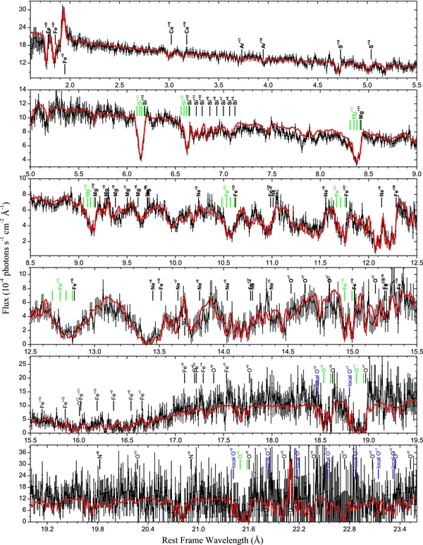
Figure 4. Chandra HETGS spectrum of NGC 3516 corrected for cosmological redshift (z = 0.008836) and binned to 10 mÅ. The red line is the best-fit model including all four velocity components. Ions producing the strongest absorption (emission) lines and blends are marked above (below) the data. Blue labels represent the local component. Green labels represent the different velocity components for a few prominent lines.
Download figure:
Standard image High-resolution image3.3. AMD Method
The large range of ionization states present in the absorber implies that the absorption arises from gas that is distributed over a wide range of ionization parameter ξ. Throughout this work, we use the following convention for the ionization parameter ξ = L/(nHr2) in units of erg s−1 cm, where L is the ionizing luminosity, nH is the H number density, and r is the distance from the ionizing source. We apply the AMD analysis in order to obtain the total hydrogen column density NH along the line of sight. The AMD can be expressed as

and
The relation between the ionic column densities Nion and the AMD is then expressed as

where Nion is the measured ion column density, Az is the element abundance with respect to hydrogen assumed to be constant throughout the absorber, and fion(log ξ) is the fractional ion abundance with respect to the total abundance of its element. We aim at recovering the AMD for the different kinematic components of NGC 3516.
For the AMD, we seek a distribution  that after integration (Equation (5)) will produce all of the measured ionic column densities. In this procedure, one must take into account the full dependence of fion on ξ. We employ the XSTAR code (Kallman & Bautista 2001) version 2.1kn3 to calculate fion(log ξ) using the continuum derived in Section 3.1, and extrapolated to the range of 1–1000 Ryd. During the fit, the AMD bin values are the only parameters left free to vary. The AMD errors are calculated by varying each bin from its best-fit value while the whole distribution is refitted. This procedure is repeated until Δχ2 = 1. The fact that changes in the AMD in one bin can be compensated by varying the AMD in other bins dominates the AMD uncertainties. This is what limits the number of bins and the AMD resolution in ξ or T. Indeed, we choose the narrowest bins (in log ξ) that still give meaningful errors. AMD in neighboring, excessively narrow bins cannot be distinguished by the data, i.e., different narrow-bin distributions produce the measured Nion values to within the errors. More details on the AMD binning method and error calculations can be found in Holczer et al. (2007).
The current method obtains a well-defined distribution of ionization, which is tightly constrained by the data, instead of the more traditional method, which constructs a superposition of individual ionization components that are δ functions of ξ, and are obtained through a global-fitting procedure. The current method should not be viewed as an upgraded version of the traditional one. In fact, the two approaches are fundamentally different. While the AMD is a bottom-up approach that uses directly measured quantities Nion to derive the distribution, global fitting uses a top–bottom method that imposes a physical model and obtains its best-fit parameters.
The advantage of the AMD method is that it helps identify column density and ionization trends that can then be compared with models (e.g., Fukumura et al. 2010), as well as the precise temperature boundaries between different phases of the possibly multi-phase absorber, e.g., due to thermally unstable temperatures (Holczer et al. 2007). It is not intended to, and indeed does not necessarily provide a superior statistical fit to the spectra.
3.4. Narrow Emission Lines
The present NGC 3516 spectrum has a few narrow, bright emission lines. The emission component is added only after the continuum is set and the absorption fit is completed. O+6 Kα and Ne+8 Kα forbidden lines are well fitted with a simple Gaussian broadened by 235 km s−1 FWHM (σ = 100 km s−1) while Fe Kα lines were fitted with a broader Gaussian of 3500 km s−1 FWHM (σ = 1500 km s−1). All lines are found to be stationary to within ≈ 100 km s−1. The centroid wavelength and photon flux are measured for each line and listed in Table 3.
Table 3. Narrow Emission Linesa
| Line | λRest | λObservedb | Flux |
|---|---|---|---|
| (Å) | (Å) | (10−5 photon s−1 cm−2) | |
| Fe+0–Fe+9 Kα | 1.94 | 1.936 ± 0.01 | 3.3 ± 0.6 |
| Fe+10–Fe+16 Kα | 1.93–1.94c | ||
| Ne+8 forbidden | 13.698 | 13.69 ± 0.01 | 0.5 ± 0.1 |
| O+6 forbidden | 22.097 | 22.093 ± 0.01 | 6 ± 1 |
Notes. aFWHM = 235 km s−1 applied uniformly to oxygen and neon emission lines. FWHM = 3500 km s−1 was applied to iron Kα emission line. bIn the AGN rest frame. cDecaux et al. (1995).
Download table as: ASCIITypeset image
4. RESULTS
4.1. Ionic Column Densities
The best-fit ionic column densities are listed in Table 4 and the resulting model is plotted over the data in Figure 4. The errors for the ionic column densities were calculated in the same manner as in Holczer et al. (2007). It can be seen that both components 1 and 2 have a wide range of ionization parameter. They both have similar absorption with ionic column densities of the order of 1016 to 1017 cm−2 in iron, silicon, neon, and magnesium, while those of the more abundant O ions are higher and reach ∼1018 cm−2. Components 1 and 2 are similar in the amount of absorption, even though component 2 seems to have slightly higher column densities. Components 3 and 4 consist exclusively of high-ionization species, mostly K-shell ions of Ne, Mg, Si, Fe, S, Ar, and even Ca. In Fe, we detect only the highest ionization L-shell ions in these fast components (see Figure 3).
Table 4. Current Best-fit Column Densities for Ions Detected in the 2006 HETGS Spectrum of NGC 3516
| Ion | Column Density | Column Density | Ion | Column Density | Column Density | |||||
|---|---|---|---|---|---|---|---|---|---|---|
| Nion | Nion | Nion | Nion | |||||||
| (1016 cm−2) | (1016 cm−2) | (1016 cm−2) | (1016 cm−2) | |||||||
| Comp1 | Comp2 | Comp3 | Comp4 | Comp1 | Comp2 | Comp3 | Comp4 | |||
| N+6 | 10+40− 1 | 50+200− 5 | ... | ... | S+14 | 2.0+2.3− 0.9 | 3.0+0.8− 2.1 | 3.5+1.1− 2.0 | ... | |
| O+0 | 8.0+2.0− 8.0 | 4.0+1.9− 4.0 | ... | ... | S+15 | 6.0+4.1− 1.8 | 5.0+1.9− 3.6 | 8.0+7.0− 1.5 | ... | |
| O+1 | 5.0+4.2− 4.0 | 6.0+2.0− 6.0 | ... | ... | Ar+16 | 3.0+1.8− 1.7 | ... | ... | ... | |
| O+2 | 3.0+3.9− 1.7 | 2.0+4.9− 2.0 | ... | ... | Ar+17 | 3.0+4.3− 2.1 | ... | 5.0+6.0− 1.8 | ... | |
| O+3 | 11+3− 11 | 2.0+2.7− 2.0 | ... | ... | Ca+18 | ... | ... | 5.0+2.6− 2.9 | ... | |
| O+4 | 5.0+1.1− 5.0 | 3.0+0.7− 3.0 | ... | ... | Ca+19 | 2.0+6.6− 2.0 | 4.0+4.0− 4.0 | 8.0+4.3− 5.0 | ... | |
| O+5 | 4.0+1.4− 3.7 | 2.0+0.4− 2.0 | ... | ... | Fe+1 | 0.2+0.4− 0.2 | 0.2+0.4− 0.2 | ... | ... | |
| O+6 | 10+90− 1.0 | 20+80− 2.0 | ... | ... | Fe+2 | 0.2+0.3− 0.2 | 0.2+0.3− 0.2 | ... | ... | |
| O+7 | 18+300− 2 | 100+300− 10 | ... | ... | Fe+3 | 0.2+0.3− 0.2 | 0.2+0.3− 0.2 | ... | ... | |
| Ne+3 | 1.0+1.9− 1.0 | 4.0+4.0− 2.0 | ... | ... | Fe+4 | 0.2+0.2− 0.2 | 0.2+0.4− 0.2 | ... | ... | |
| Ne+4 | 3.0+5.5− 1.0 | 0.5+3.2− 0.5 | ... | ... | Fe+5 | 0.2+0.3− 0.2 | 0.2+0.3− 0.2 | ... | ... | |
| Ne+5 | 4.0+1.7− 2.5 | 3.0+0.8− 2.5 | ... | ... | Fe+6 | 0.2+0.3− 0.2 | 0.2+0.3− 0.2 | ... | ... | |
| Ne+6 | 1.0+1.3− 0.9 | 2.0+6.0− 0.4 | ... | ... | Fe+7 | 0.5+2.1− 0.1 | 2.0+1.7− 0.3 | ... | ... | |
| Ne+7 | 4.0+4.9− 0.8 | 2.0+1.1− 1.0 | ... | ... | Fe+8 | 1.0+1.0− 0.3 | 2.0+2.7− 0.3 | ... | ... | |
| Ne+8 | 4.0+18− 0.4 | 6.0+25− 0.6 | 2.0+2.0− 0.2 | ... | Fe+9 | 1.0+5.1− 0.2 | 3.8+1.7− 0.7 | ... | ... | |
| Ne+9 | 7+30− 0.4 | 13+50− 1.3 | 7.0+30− 0.7 | 4.0+18− 0.6 | Fe+10 | 0.5+1.7− 0.4 | 4.0+1.7− 0.6 | ... | ... | |
| Mg+4 | 0.5+2.4− 0.5 | 0.5+1.1− 0.5 | ... | ... | Fe+11 | 1.7+0.8− 0.7 | 1.4+1.2− 0.6 | ... | ... | |
| Mg+5 | 0.5+0.8− 0.5 | 0.5+6.8− 0.2 | ... | ... | Fe+12 | 1.0+1.0− 0.2 | 2.0+0.4− 0.7 | ... | ... | |
| Mg+6 | 1.5+2.5− 0.4 | 0.9+3.7− 0.3 | ... | ... | Fe+13 | 0.5+0.3− 0.4 | 1.0+0.3− 0.4 | ... | ... | |
| Mg+7 | 1.5+3.0− 0.2 | 0.8+5.2− 0.1 | ... | ... | Fe+14 | 0.5+0.1− 0.4 | 0.5+0.2− 0.2 | ... | ... | |
| Mg+8 | 2.0+2.9− 0.2 | 2.0+0.5− 0.6 | ... | ... | Fe+15 | 0.2+0.4− 0.2 | 0.5+1.3− 0.1 | ... | ... | |
| Mg+9 | 2.0+1.8− 0.3 | 1.5+3.5− 0.2 | ... | ... | Fe+16 | 2.4+0.5− 0.5 | 2.5+1.6− 0.3 | ... | ... | |
| Mg+10 | 4.0+9.4− 0.4 | 4.0+20− 0.4 | 2.0+8.0− 0.2 | 1.0+3.2− 0.1 | Fe+17 | 2.5+0.2− 2.2 | 2.5+0.6− 0.7 | 3.0+0.5− 0.7 | 1.5+1.6− 0.2 | |
| Mg+11 | 5.5+1.9− 0.6 | 9.0+5.6− 0.4 | 6.5+3.7− 0.7 | 2.5+2.8− 0.3 | Fe+18 | 5.0+0.5− 1.2 | 6.0+1.6− 0.5 | 4.4+0.8− 0.7 | 1.3+0.8− 0.4 | |
| Si+5 | 3.0+10− 0.8 | 4.0+9.4− 0.8 | ... | ... | Fe+19 | 3.6+1.0− 0.4 | 3.9+2.4− 0.4 | 4.2+1.1− 0.5 | 2.0+0.6− 0.2 | |
| Si+6 | 3.0+3.2− 0.8 | 4.0+4.5− 0.6 | ... | ... | Fe+20 | 2.2+2.2− 0.2 | 3.5+8.8− 0.4 | 2.8+9.6− 0.3 | 1.0+2.4− 0.2 | |
| Si+7 | 2.0+4.7− 0.3 | 3.0+2.3− 0.6 | ... | ... | Fe+21 | 3.0+3.0− 0.3 | 3.5+4.5− 0.4 | 2.7+3.5− 0.3 | 0.7+2.7− 0.1 | |
| Si+8 | 3.0+2.8− 0.3 | 4.0+2.7− 0.4 | ... | ... | Fe+22 | 3.0+3.7− 0.3 | 3.0+7.9− 0.3 | 3.0+4.5− 0.3 | 0.5+1.0− 0.3 | |
| Si+9 | 2.0+1.2− 0.4 | 5.0+0.6− 0.9 | ... | ... | Fe+23 | 0.3+8.0− 0.2 | 4.0+12− 0.4 | 8.0+4.5− 0.8 | 2.0+0.6− 2.0 | |
| Si+10 | 2.6+0.6− 0.5 | 2.9+1.0− 0.3 | ... | ... | Fe+24 | 0.1+40− 0.1 | 30+70− 12 | 22+66− 14 | 20+25− 13 | |
| Si+11 | 2.5+0.8− 0.5 | 2.8+2.0− 0.3 | ... | ... | Fe+25 | 0.1+50− 0.1 | 10+70− 10 | 60+150− 20 | 130+500− 36 | |
| Si+12 | 4.5+0.9− 0.7 | 7.0+1.8− 0.7 | 1.5+2.5− 0.2 | 1.5+0.9− 0.4 | ||||||
| Si+13 | 4.7+4.3− 0.4 | 15+7.7− 1.5 | 14+6.8− 1.4 | 5.0+3.4− 0.5 | ||||||
Download table as: ASCIITypeset image
4.2. AMD for Components 1 and 2
The best-fit AMD for components 1 and 2 in NGC 3516 is presented in Figure 5 and the integrated column density is presented in the bottom panel of Figure 5. These AMDs were obtained using 21 charge states of Fe from Fe+3 through Fe+23. K-shell Fe is heavily blended for all the kinematic components (1 through 4); however most of the absorption is due to components 3 and 4. Many M-shell ions are only tentatively detected. Nonetheless, the strict upper limits on so many Fe ions provide tight constraints on the AMD around where these ions form. The result of Figure 5 is enabled by the AMD method and, obviously, cannot be as well quantified with a standard multi-ξ fit. The current integrated AMD of the absorber in NGC 3516 (Figure 5) gives a total column density of NH = (1.8 ± 0.5) × 1022 cm−2 for component 1 and NH = (2.5 ± 0.3) × 1022 cm−2 for component 2.
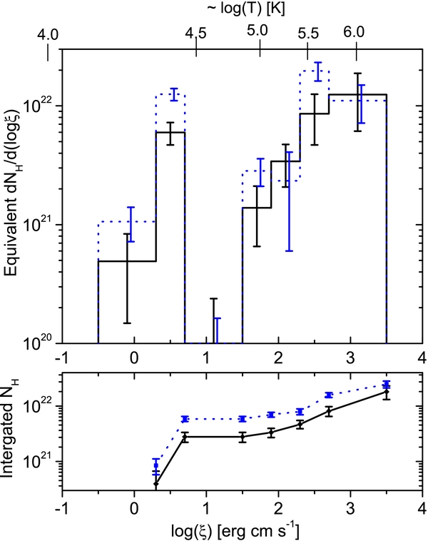
Figure 5. AMD of component 1 (solid black) and component 2 (dashed blue) in the outflow of NGC 3516, obtained exclusively from Fe absorption and scaled by the solar Fe/H abundance of 3.16 × 10⁻⁵ (Asplund et al. 2009). The corresponding temperature scale, obtained from the XSTAR computation, is shown at the top of the figure. The accumulative column density up to ξ is plotted in the lower panel, yielding a total of NH = (1.8 ± 0.5) × 1022 cm−2 for component 1 and NH = (2.5 ± 0.3) × 1022 cm−2 for component 2.
Download figure:
Standard image High-resolution imageBoth AMDs feature a statistically significant minimum at 0.7 < log ξ < 1.5 (erg s−1 cm), which corresponds to temperatures 4.5 < log T < 5 (K). This discontinuity in the AMD at the same temperatures was also observed in IRAS 13349+2438, NGC 3783 (Holczer et al. 2007), NGC 7469 (Blustin et al. 2007), and MCG –6–30–15 (Holczer et al. 2010). Indeed, the multi-phase nature of AGN outflows is found in many warm absorbers (Sako et al. 2001; Krongold et al. 2003, 2005, 2007; Detmers et al. 2011). It is mostly a manifestation of the relatively low ionic column densities observed for the ions Fe+11– Fe+15, as can be seen in Table 4. One way to explain this gap is that this temperature regime is thermally unstable (Holczer et al. 2007; Gonçalves et al. 2010). Gas at 4.5 < log T < 5 (K) could be unstable as the cooling function Λ(T) generally decreases with temperature in this regime. Such instabilities could result in a multi-phase (hot and cold) plasma in pressure equilibrium, as suggested by Krolik et al. (1981).
It is somewhat surprising that the AMDs of components 1 and 2 are so similar, which implies the physical conditions in components 1 and 2, the distance from the source and the outflow density, as well as the overall outflow column are similar. Given the similar AMDs we are led to think that these components are connected. What about the faster components 3 and 4? Are they also connected to components 1 and 2? Components 3 and 4 have yet to be reported, so no comparisons can be made with other authors. These new components and a plausible geometric explanation are addressed in detail in Section 4.7, while their ionization distributions are discussed below.
4.3. AMD for Components 3 and 4
The best-fit AMD for components 3 and 4 in NGC 3516 is presented in Figure 6 and the integrated column density is presented in the bottom panel of Figure 6. The black line represents component 3 while the blue dotted line represents component 4. These AMDs were obtained using L-shell and K-shell charge states of Fe only as no M-shell Fe ions are detected, which is why these AMDs begin at log ξ = 2 (erg s−1 cm). On the other hand, the AMD value of these components for log ξ > 2 (erg s−1 cm) is an order of magnitude higher than in components 1 and 2. In the K-shell Fe lines, all the components are blended; however the troughs are dominated by components 3 and 4. It can be seen that both AMDs show similar shape but component 4 has a minimum at 2.8 ⩽ log ξ ⩽ 3.4 (erg s−1 cm), mostly due to the low columns of Fe+20–Fe+22, as can be seen in Table 4. Similarly to components 1 and 2, we are led to think that components 3 and 4 are also connected; particularly since they both appear in the 2006 spectrum, but are both absent in the 2001 spectrum (see Section 4.6). The total column density (integrated AMD) gives NH = (6.9 ± 4.3) × 1022 cm−2 for component 3 and NH = (5.4 ± 1.2) × 1022 cm−2 for component 4.

Figure 6. AMD of component 3 (black) and component 4 (dashed blue) in the outflow of NGC 3516 obtained exclusively from Fe absorption and scaled by the solar Fe/H abundance of 3.16 × 10⁻⁵ (Asplund et al. 2009). The corresponding temperature scale, obtained from the XSTAR computation, is shown at the top of the figure. The accumulative column density up to ξ is plotted in the lower panel, yielding a total of NH = (6.9 ± 4.3) × 1022 cm−2 for component 3 and NH = (5.4 ± 1.2) × 1022 cm−2 for component 4.
Download figure:
Standard image High-resolution image4.4. Total Column Density
In order to further compare our results with previous outflow models for NGC 3516, we can formally rebin the AMD in Figure 5 to two regions, one below log ξ < 0.5 and one above log ξ > 1.5 (this process is done to each kinematic component). The physical parameters of these two ionization regions are subsequently compared with all previous works in Table 5.
Table 5. Physical Parameters for Absorption Components in Order of Outflow Velocity: Comparison
| Ref.a | Observatory | Component | Outflow | Column | Total Column | Ionization |
|---|---|---|---|---|---|---|
| Velocity | Density | Density | Parameter | |||
| (km s−1) | (1021 cm−2) | (1021 cm−2) | log ξ (erg s−1 cm) | |||
| 1 | ASCA | 1 | <−120 | 14.1 ± 3.9 | 21 ± 4 | 1.66 ± 0.31b |
| 2 | <−120 | 6.9 ± 0.6 | 0.32 ± 0.11b | |||
| 2 | ASCA | ... | 10.0+1.1− 1.6 | 10 ± 1 | 1.44 ± 0.03 | |
| 3 | ROSAT | −500 | 7 ± 1 | 7 ± 1 | 0.90–1.11b | |
| 4d | BeppoSAX | Warm | −500 | 10 ± 0.4 | 168 ± 73 | 0.73 ± 0.10b |
| Hot | −500 | 158 ± 73 | 2.36 ± 0.10b | |||
| 5e | ASCA | ... | 8 | 8 | −2.6c | |
| 6 | XMM-Newton | UV | −200 | 6 ± 2 | 272 ± 23 | −0.5 |
| Chandra | High | −1100 | 16 | 2.5 | ||
| Heavy | −1100 | 250 ± 23 | 3.0 | |||
| 7 | Suzaku | Primary | ... | 55 ± 2 | 95 ± 45 | 0.3 ± 0.1 |
| High Ion. | −1100 | 40+46− 31 | 3.7+0.3− 0.7 | |||
| Zone 1 | ... | 2.4+0.3− 0.2 | 467 ± 110 | −2.43+0.58− 0.03 | ||
| 8 | XMM-Newton | Zone 2 | ... | 0.5 ± 0.1 | 0.25 | |
| Chandra | Zone 4 | −1000 | 262+63− 87 | 4.31+1.19− 0.14 | ||
| Zone 3 | −1600 | 202+87− 32 | 2.19 ± 0.07 | |||
| 9 | XMM-Newton | A | −100 | 4 | 34 | 0.9 |
| C | −900 | 10 | 3.0 | |||
| B | −1500 | 20 | 2.4 | |||
| 10 | Chandra | Comp 1 | −350 ± 100 | 2.8 ± 0.6 | 166 ± 45 | −0.5–0.7 |
| −350 ± 100 | 15.3 ± 5.0 | 1.5–3.5 | ||||
| Comp 2 | −1500 ± 150 | 5.9 ± 0.6 | −0.5–0.7 | |||
| −1500 ± 150 | 18.8 ± 3.5 | 1.5–3.5 | ||||
| Comp 3 | −2600 ± 200 | 69 ± 43 | 2–4 | |||
| Comp 4 | −4000 ± 400 | 54 ± 12 | 2–4 |
Notes. a(1) Kriss et al. 1996b; (2) Reynolds 1997; (3) Mathur et al. 1997; (4) Costantini et al. 2000; (5) Netzer et al. 2002; (6) Turner et al. 2005; (7) Markowitz et al. 2008; (8) Turner et al. 2008; (9) Mehdipour et al. 2010; (10) present work. bIonization parameter used is U. cIonization parameter used is UOx. dReference to data set 97BF therein. eReference to data set ASCA98 therein.
Download table as: ASCIITypeset image
The total column density that we find for the low velocity −350 km s−1 component 1 is roughly 2 × 1022 cm−2 and is comparable to that of Kriss et al. (1996b) (their components 1 and 2). Most other works are consistent with this result to within a factor of two (Reynolds 1997; Mathur et al. 1997; Netzer et al. 2002; Turner et al. 2005, 2008; Mehdipour et al. 2010). However, if the Costantini et al. (2000) hot component also refers to our component 1, then there is a larger disagreement of around an order of magnitude.
Component 2 (v = −1500 km s−1) was detected only with the more recent grating instruments. The column density we find for component 2 is in good agreement with the Turner et al. (2005) "High" component and the Mehdipour et al. (2010) component "B" and still consistent with the weak constraints of Markowitz et al. (2008). It is an order of magnitude lower than Turner et al. (2008) "Zone 3" and "Zone 4" and the Turner et al. (2005) "Heavy" component. We should note that both Turner et al. (2008) and Mehdipour et al. (2010) used another component with an intermediate outflow velocity (∼−1000 km s−1), namely "Zone 4" and component "C," respectively. Table 5 shows that the total column density can vary between observations and authors by nearly two orders of magnitude. The highest column densities are due to few spectral features, e.g., Fe–K in the present work, or to the need to explain spectral curvature with photoelectric absorption without lines (Turner et al. 2008). The diversity in ionization parameter and velocity is mostly due to selective identification of spectral features. Our analysis shows that a broad range of both ionization and velocity are present.
4.5. Possible Local Absorption
The outflow velocity of component 3 is −2600 ± 200 km s−1 matching the cosmological recession of −2650 km s−1, which raises the possibility that some of the absorption at this velocity is due to local absorption as commonly found along lines of sight to bright AGNs (e.g., Nicastro et al. 2003; Williams et al. 2005). A similar component was recently found in MCG –6–30–15 (Holczer et al. 2010), although there it was kinematically resolved (−1900 ± 150 km s−1 versus −2300 km s−1). The oxygen and nitrogen lines of component 3 are narrow and thus suspect of having a local origin. These lines require vturb = 100 km s−1 (FWHM = 170 km s−1), which is less than vturb = 300 km s−1, which is used for higher ionization. This narrow width is consistent with local, ionized interstellar medium (ISM) UV absorption lines along this line of sight (Kraemer et al. 2002). There are a few additional reasons to favor the local component scenario for O and N. First, they form at lower ionization parameters of log ξ ∼ 0–2, while most of component 3 is primarily comprised of high ionization species. In Fe, we do not detect any M-shell ions, and not even Fe+16 in this component. Even though we cannot conclusively determine whether the oxygen and nitrogen absorption comes from outflow component 3, or has a local origin, we tend to favor the local origin scenario because such a component is often observed.
The (presumably) local component column densities are shown in Table 6. The low charge states are due to the Galactic disk and halo, and likely not associated with the higher ionization states that are due to the hot phase of the Galactic halo or the Local Group. The oxygen ionic column densities are all in the range of several 1016 cm−2, which implies a neutral hydrogen column density of a few 1020 cm−2, using 4.9 × 10⁻⁴ for the O to H ratio (Asplund et al. 2009) and a fractional ionic abundance of 0.5. This value is consistent with the Galactic absorption of NH = 3.23 × 1020 cm−2 (Dickey & Lockman 1990). Using the same calculations for N+6 gives a slightly higher neutral hydrogen column density of the order of ∼1021 cm−2.
Table 6. Oxygen and Nitrogen Ionic Column Densities at z = 0
| Charge | Nion Local | λRest |
|---|---|---|
| State | (1016 cm−2) | (Å) |
| N+6 | 20+50− 2 | 19.825,20.911 |
| Neutral O | 4.0+8.0− 4 | 23.523 |
| O+1 | 6.0+20− 2.7 | 23.347 |
| O+2 | 4.0+11− 3.8 | 23.071 |
| O+3 | 3.0+1.3− 3.0 | 22.741 |
| O+4 | 1.5+1.5− 1.5 | 22.374 |
| O+5 | 1.0+0.6− 1.0 | 22.019 |
| O+6 | 5+20− 0.5 | 21.602 |
| O+7 | 10+40− 1 | 18.969 |
Download table as: ASCIITypeset image
Note that most species of component 3 are likely not local since their ionization and column densities are too high. Ions such as Fe+23 − +25, K-shell S and Si (see Table 4) are usually not observed in the local ionized ISM. Moreover, the high column density measured in this component of NH ∼ 1023 cm−2 is far higher than typical local ISM columns.
4.6. Variability
The observation of 2006 caught NGC 3516 in a much higher state than the 2001 observation, as can be seen in Figure 2. So far, the analysis in this paper has focused on the 2006 observation. We now want to use the two flux states to study the differences between the two. Several explanations for the flux and spectral variability of NGC 3516 can be found in the literature. Netzer et al. (2002) reported a slow, monotonic decay in flux between 1994 and 2000; however BeppoSAX observations from 1996 and 1997 as well as the present data show a sharp transition between high and low flux over a period of four months (see Table 1). Turner et al. (2005, 2008) used a varying covering factor. However, Mehdipour et al. (2010) found that a varying covering factor did not fit the data, while a variable source continuum could.
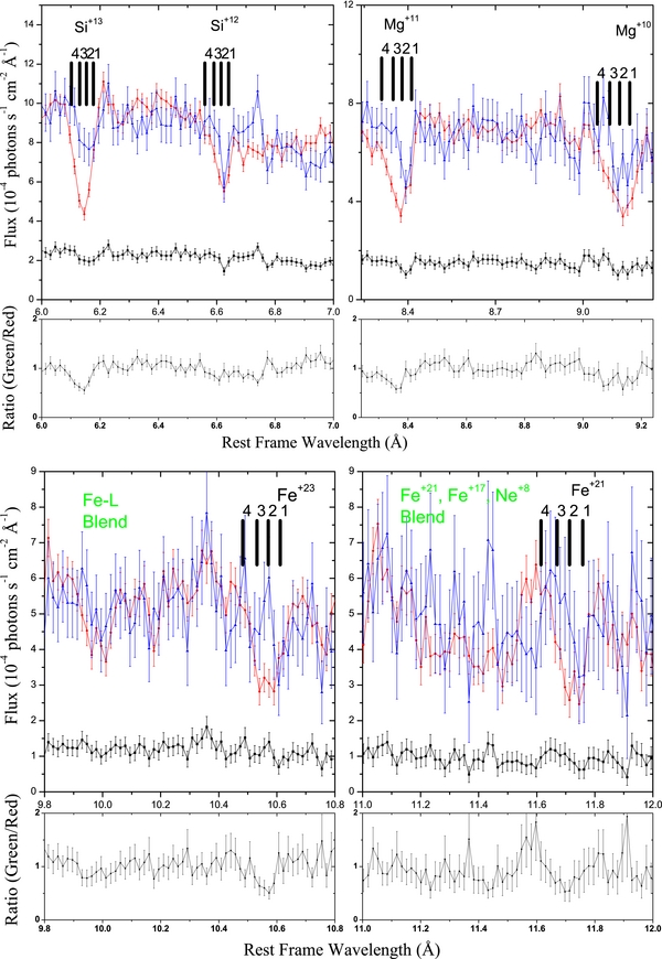
In order to compare the absorption in 2001 and 2006 we scaled up the 2001 spectrum to the flux level of 2006 near specific lines. Since absorption depends exponentially on optical depth, this comparison shows changes in optical depth directly, independent of continuum flux. If the absorber did not change, the scaled-up trough should match that of the high state. Because the continuum shape during the two states is different, this comparison is meaningful only locally. Indeed, we show this comparison around the most prominent lines. Results for Si and Mg Kα lines and for Fe+23 and Fe+21 are shown in Figure 7, where the low statistics spectrum is multiplied by 4 in the upper left panel, by 4.5 in the upper right panel, by 4.3 in the lower left panel, and by 5.2 in the lower right panel. The signal-to-noise ratio (S/N) in the low state is worse, but it appears that component 1 (the slowest component) did not change much between the high and low states. On the other hand, some of component 2 and most of components 3 and 4 are absent in the 2001 low state. In the next section, we discuss a possible geometrical explanation for this result.
Figure 7. Chandra HETGS spectrum of NGC 3516 corrected for cosmological redshift (z = 0.008836) around K-shell Si (upper left panel), K-shell Mg (upper right panel), Fe+23 (lower left panel), and Fe+21 (lower right panel) lines. The black and red spectra represent the combined observations of 2001 and 2006, respectively. The blue data represent the 2001 spectrum scaled up to match the 2006 continuum. The four kinematic components are labeled. The spectral lines in the 2001 data lack absorption in the fast component that is present in 2006. The lower panels are the ratios between the 2006 and 2001 scaled spectra.
Download figure:
Standard image High-resolution image
4.7. Possible Geometry of Outflow
We find that, apart from a lower continuum level, the 2001 spectrum of NGC 3516 also lacks the faster absorption components. The appearance of high ionization (log ξ ∼ 3.5 erg s−1 cm) components with columns of NH ∼ 1023 cm−2 is reminiscent of the variable covering invoked by Turner et al. (2005, 2008) to explain the varying continuum shape. We allude to three other possible explanations.
- 1.Photoionization change. The faster components of the outflow are also more ionized. One possibility could be that the fast components recombined due to the reduced flux and are thus not seen in 2001. However, one would still expect to observe the fast components in lower charge states. We could not detect the fast components in the 2001 spectrum in any ion. Since the 2001 spectrum has a much lower S/N, we cannot unambiguously rule out this possibility.
- 2.Fast components crossing line of sight. Another possibility could be that the fast components, while not in the line of sight in 2001, passed through our line of sight in 2006: 5 years are plenty of time, compared to the variability timescale of months that perhaps represents the size of the source, to make this scenario work. Such transverse velocities have been proposed for NGC 4151 by Kraemer et al. (2006). Recent simulations show this behavior of disappearing fast absorbing component explicitly on a similar timescale of few years (Sim et al. 2010, Figure 7).
- 3.Lighting up the disk. The third possibility is that the fast components are present the whole time, but in 2001, when the flux is low, there was no light from the accretion disk behind them for them to absorb. In 2006, the source flux is much brighter, whether intrinsic source output change or flux change due to variable covering factor by thick gas, which could result from a flare on the disk that illuminates the fast components from behind, and which subsequently they absorb along the line of sight.
With the current spectra, one cannot rule out any of these scenarios. With better S/N spectra, one might be able to confirm (or rule out) changes in the (photo)ionization state if the fast component is detected (or not detected) in low ionization species during the low flux state. If one would detect a change in the covering fraction in the narrow absorption lines, which we are not able to detect here, that would be evidence for transverse velocities (Kraemer et al. 2006). The possibility of flaring on the disk is most difficult to test, as the angular resolution required for detecting sources on sub-disk scales is currently prohibitive.
5. CONCLUSIONS
We have analyzed the kinematic and thermal structure of the ionized outflow in NGC 3516. We find absorption troughs in dozens of charge states that extend from zero to almost 5000 km s−1. We model the outflow with four absorption systems. The first and second components are outflowing at −350 and −1500 km s−1, and span a considerable range of ionization from at least Fe+1 to Fe+23 (−0.5 < log ξ < 3.5 (erg s−1 cm)). The third and fourth components are outflowing at −2600 and −4000 km s−1, respectively, and are highly ionized featuring only L-shell and K-shell iron and K-shell ions from lighter elements. Finally, a component of local absorption at z = 0 (−2630 km s−1) is detected: this component could be part of the third component; however its low ionization and narrow time profiles imply it is more likely at z = 0.
Using our AMD reconstruction method for all four components, we measured the distribution of column density as a function of ξ. We find a double-peaked distribution with a significant minimum at 0.7 < log ξ < 1.5 (erg s−1 cm) in components 1 and 2, which corresponds to temperatures of 4.5 < log T < 5 (K). This minimum was observed in other AGN outflows like MCG –6–30–15, NGC 3783, IRAS 13349+2438, and NGC 7469, and it can be ascribed to thermal instability that appear to exist ubiquitously in photoionized Seyfert winds. The AMD of component 3 shows a continuous rise in column density toward higher ionization parameters. The AMD of component 4 is similar in some aspects to that of component 3; however it shows a minimum at log T ∼ 6 (K) mostly due to low Fe+20–Fe+22 column densities. The local absorption system could arise from either the ionized Galactic ISM or from the Local Group. The fast components 3 and 4 are not present in the lower flux spectra of 2001.
We thank Shai Kaspi for useful comments. This work was supported by a grant from the ISF.