


ABSTRACT
Voyager 1 has observed strong increases in the intensities of 2–160 MeV electrons since crossing the termination shock of the heliosphere in 2004 December. Before this time these intensities were submerged below the detector background, except for occasional transient events. These increases are large compared to the concurrent increases of positive ions such as H, He, and O. A significant part is probably due to temporal effects as the heliosphere was recovering to solar minimum conditions from 2005 to early 2010. The intensity observed by Voyager 2 since its crossing of the shock in 2007 September is 5–10 times lower than that observed by Voyager 1, which is so low that the electron intensity may still be below the background produced by high-energy protons in the detector. This points to a large north–south asymmetry in the properties of the heliosheath. It is shown that the observations suggest that these electrons are not freshly accelerated on the termination shock, but rather that they are of galactic origin—while they may be re-accelerated by that shock. In this paper, these intensities are modeled with numerical solutions of the cosmic-ray transport equation. It is shown that because they are relativistic, the electrons are much more sensitive to the form of the diffusion coefficient at low rigidities than ions, and that this can explain the asymmetry.
Export citation and abstract BibTeX RIS
1. INTRODUCTION
In Caballero-Lopez et al. (2004), we studied the modulation of galactic cosmic-ray (GCR) protons and helium nuclei (H and He) throughout the heliosphere. We emphasized the modulation effects in the vicinity of the termination shock (TS) of the solar wind (SW) and in the heliosheath beyond this shock. In that paper, we made the point that one can claim a satisfactory understanding of the modulation if the energy spectra observed at widely different positions in the heliosphere and different energies can be explained simultaneously. This paper contains such a comprehensive study of cosmic-ray electrons in the heliosheath, with the important constraint that the electron intensity observed at Earth must be explained at the same time.
These electrons may originate from several sources. Below ∼200 MeV, GCR electrons are the source of the lower-energy diffuse gamma and X-ray emission from the galaxy, and may play a major role in ionizing and heating the interstellar medium. These lower-energy electrons are produced as knock-on electrons, as well as directly accelerated primaries and interstellar secondaries from the decay of charged pions. When combined, these processes produce what is called the electron local interstellar spectrum (LIS). This spectrum can be observed through its radio synchrotron emission as described by, e.g., Strong et al. (2000), Webber & Higbie (2008), and references therein. Two estimates of this LIS are shown in Figure 1. Other spectra lie between these limits. The spectrum marked Webber and Higbie IS-7 will be used in this paper.

Figure 1. Electron local interstellar spectra from Webber & Higbie (2008). The spectrum IS-7 of Webber & Higbie (2008) was chosen in this work because it gives the lowest realistic intensity in the interval 100–1000 MeV. The stars are from radio observations by Peterson et al. (1999). V1, V2, and 1 AU electron intensities are shown for comparison.
Download figure:
Standard image High-resolution imageThe cosmic-ray subsystems (CRS) on Voyagers 1 and 2 measure the intensity of these electrons from 2.5 to 160 MeV. The high-energy telescope (HET) responds to electrons from 2.5 to 10 MeV, and the electron telescope to electrons from 6 to 160 MeV. At the same time it also measures the H intensity in the range 1.8–300 MeV, and He from 1.8 to 650 MeV n−1. Figure 2 shows these observed counting rates in six different energy channels, uncorrected for background. Except for periods when there were large fluxes of electrons of Jovian or solar origin, the responses of these telescopes inside the TS have been dominated by the background produced by high-energy protons. This background level is represented by the intensities from 1997 to approximately 2002. However, at about the time when V1 crossed the TS, on 2004 December 16 at 94 AU, the true electron intensity started to emerge above this background. (They were first seen at energies below 30 MeV as the so-called TS particle (TSP) events from ∼85 AU outward, associated with the passage of strong transients, e.g., McDonald et al. 2006.) By early 2010, V1 had progressed at least 18 AU into the heliosheath beyond the shock, and it has seen strongly increasing electron intensities up to then.
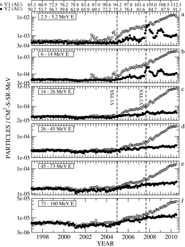
Figure 2. Electron intensities in six energy channels as observed by V1 and V2 from 1997 to early 2010. Crossings of the TS are indicated. Prior to 2002 the electron channels counted only the proton-induced background. Since the shock crossing the V1 intensities have increased steadily at a rate of ∼50% per year, but the V2 increases are much smaller.
Download figure:
Standard image High-resolution imageThe situation is entirely different on V2 since its crossing of the TS on 2007 August 30 at 84 AU. Although the three lowest energy channels, below 30 MeV, saw two events with strong increases in early 2008 and early 2009 that resemble the TSP events seen by V1 in 2002 and 2004, the overall increases have been much smaller than on V1, resulting in a difference of about a factor of 10 between the two Voyager intensities by early 2010. For comparison, the V2 increases in the low-rigidity range P = 2 to 160 MV are as small as the increase in the high-rigidity 265 MeV n−1 (P = 1.3 GV) He, which suggests that the V2 intensity in the heliosheath is also mainly background.
In Figure 3, this background is subtracted from the electron intensities as discussed in McDonald (2007). It shows that after 2005.5 all the V1 channels increase at a steady rate of ≈90% per year, independent of rigidity over two decades from 2 to 160 MV. This is a strong indication that the diffusion coefficient must be independent of rigidity in this interval. On the other hand, the V2 channels only see a much lower, highly fluctuating intensity, especially below 30 MeV, with little indication of a steady increase.
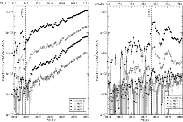
Figure 3. Intensities in four of the channels of Figure 1, corrected for background. All the V1 channels show an increase of ≈90% per year, independent of energy.
Download figure:
Standard image High-resolution imageSuch a difference between the two spacecraft can be due to two reasons, namely a radial gradient due to the fact that V1 is 21 AU further out than V2, or a latitudinal gradient because V1 is at 34° north of the ecliptic plane, and V2 at 29° south. In the case of a "radial explanation" the data points for 2010 in Figure 3 imply that the radial gradient for the four channels would be between 10% and 20% per AU. It must be borne in mind, however, that a significant fraction of these increases are due to temporal effects as the heliosphere was resetting from solar maximum conditions from 2005 to early 2010. In the case of a "latitudinal explanation" the difference may be due to several observed and modeled asymmetries of the heliosheath, which were compiled by Opher et al. (2009). Generally, these asymmetries are such that they imply a narrower heliosheath with stronger magnetic fields in the southern hemisphere, i.e., at the position of V2. This different field strength and topology may lead to different turbulence spectra in the northern and southern parts of the heliosheath.
This large asymmetry between the electron intensities presents a challenge to modulation theory, because its absence from other species implies that its origin cannot be sought in an asymmetry of the SW or in the size of the heliosheath at the two latitudes of V1 and V2, because that would affect those other species equally. The only parameter that can produce this effect predominantly for electrons is a different diffusion coefficient than for the nuclear species.
Figure 4 shows V1 and V2 spectra as they were observed in the period 2010 January 1 to March 20. For comparison, it also shows the spectrum of anomalous cosmic-ray (ACR) hydrogen in 2008. The two power laws of the form T−1.5 through these spectra are drawn by hand. These spectral forms have been relatively stable since 2005.5. The figure also shows the 1 AU spectra observed during the 1986/1987 solar minimum by Huber (1998) and the 1998 solar minimum spectrum by Alcaraz et al. (2000). These 1 AU spectra are only relevant to this study down to ∼100 MeV, because at lower energies they are increasingly dominated by Jovian electrons (e.g., Ferreira et al. 2001). A second indicator that the V2 detector is still dominated by background is that the intensity in the 100 MeV channel is essentially the same as the intensity at 1 AU.
Figure 4. Electron and proton spectra observed in the heliosheath by V1 at 112 AU (closed squares), and electrons on V2 at 91 AU (open squares). Electrons observed at 1 AU during the solar minimum of 1987 are from Huber (1998, closed triangles), and in the solar minimum of 1998 from Alcaraz et al. (2000, open triangles). The stars represent the interstellar spectrum as measured by Peterson et al. (1999). The straight lines with power-law indices of −1.5 on the V1 data are drawn by hand.
Download figure:
Standard image High-resolution imageIn principle, these electrons can also originate from acceleration by several processes inside the heliosphere, such as the TS, traveling interplanetary shocks, or stochastic acceleration in the outer regions of the heliosheath. In this case they should be called anomalous electrons, in analogy to the well-known ACR component observed for several ion species. This is considered less likely, though, for two reasons. First, according to standard shock acceleration theory, e.g., Steenberg & Moraal (1999), a shock with the compression ratio s produces a distribution function f(p) ∝ p3s/(1−s) or energy spectrum j(T) ∝ p(2+s)/(1−s). Since the electrons in this energy range are relativistic (p ∝ T), while the ions are not (p ∝ T1/2), the electron spectral index should be twice as large as for the protons, but they are observed to be the same. Furthermore, the electron spectral index of −1.5 requires a shock compression ratio s = 7, while the maximum value for such a shock is s = 4, and the inferred value at the TS crossings was s∼ 2.5. The second reason is that the pool of available electrons has too low rigidity to be readily picked up by the turbulence in the initial stages of the acceleration process. For instance, ACR protons that are produced through ionization of interstellar neutrals with no kinetic energy in the stationary frame, and hence start with a speed of 400 km s−1 relative to the SW and the heliospheric magnetic field (HMF), have T = 1 keV and P = 1.4 MV in the SW frame, while electrons only have T = 0.5 eV and P = 30 V. The thermal electron pool in the SW has higher energy than this, namely T = 10 eV and P = 200 V, but this is still very low for the pick-up process of the acceleration to be effective.
These 2 to 160 MeV low-energy electrons greatly expand the useful rigidity range available for modulation studies, for two reasons. First, they are relativistic, and hence their kinetic energy, T, spans a rigidity range, P, from 2 to 160 MV. In this rigidity range, protons are non-relativistic, such that the corresponding energy range is only T = 2 keV to 10 MeV, and they are therefore very heavily modulated. Below P≈ 100 MV, these nuclei are in the adiabatic limit throughout most of the heliosphere, which fixes their kinetic energy spectrum to the form j ∝ T, and eliminates all density gradients, independent of modulation conditions and their changes. We will show in the demonstration solutions of the transport equation that the situation is entirely different for electrons. Second, at these low energies protons and He nuclei are entirely submerged below the ACR component. This ACR component extends up to about 100 MeV per nucleon, which corresponds to P = 400 MV for protons and P = 800 MV for He nuclei. Hence, GCR modulation studies are limited to rigidities P > 400 MV. (The exceptions are species such as 12C which have such low first ionization potentials that the ACR component in the heliosphere is very small.)
A constraint on low electrons is that in the inner heliosphere they are difficult to observe due to their strong modulation and the fact that the intensity at T< 50 MeV is submerged below the electron intensities produced by Jupiter, e.g., Ferreira et al. (2001). In the outer heliosphere, however, this contamination from Jovian electrons is insignificant.
This paper is mainly devoted to demonstrate the various transport effects on these electrons with numerical solutions of the transport equation, while in the last section we present the best overall explanation for the observed intensities. The conclusion is that one can understand the general features, especially that of the V1–V2 asymmetry, but that there are several details that still have to be resolved.
2. DIFFERENCE BETWEEN ELECTRON AND NUCLEI MODULATION
Electrons were not observed by the Voyagers up to the TS because they are stronger modulated than cosmic-ray nuclei, leading to a larger radial gradient, which caused them to be submerged below the detector background. They were, therefore, submerged below the background counts of high-energy nuclei. This stronger modulation is due to lower adiabatic energy losses than for the nuclei, and the source of this difference is the mass difference between the two species. Now that they are observed, however, they are much more sensitive to modulation conditions than nuclei, and hence are a much more useful probe of conditions in the heliosheath.
This underlying feature can be demonstrated by solutions of the simple steady-state, one-dimensional (spherically symmetric) approximation
of the cosmic-ray transport equation
In these equations, f is the omnidirectional distribution function in terms of momentum p, related to the (generally measured) intensity in terms of kinetic energy by j(T) = p2f(p); V is the radial SW velocity, V is its magnitude,  is the diffusion tensor containing elements parallel, perpendicular, and transverse (drifts) to the HMF, and κ is its effective scalar value in the simplified spherically symmetric case.
The three terms in Equation (1) describe convection, diffusion, and adiabatic energy loss. There is only one species-dependent quantity, which is κ = λv/3, with λ(r, P) being the diffusion mean free path at the radial distance r and rigidity P. This κ is usually written as κ = βκ1(r)κ2(P), with β = v/c. The relationship between momentum, rigidity, P, and kinetic energy per nucleon, T, is  , while
  where A and Z are the mass and charge numbers, respectively, and E0 is the rest mass. For protons and electrons, A and Z are both 1, but E0 is 938 MeV for protons and 511 keV for electrons. This E0 is the only difference between the two species that appears in the transport Equation (1). Figure 5 shows solutions of Equation (1) with κ = 7.2 × 10²²βP cm2 s−1, V = 400 km s−1, and an outer boundary rb = 150 AU. This means that κ is independent of r. The LIS was chosen as
 ![$j_{\rm LIS}=0.13 [T^2+T_k^2]^{[(\gamma _1-\gamma _2)/2]}T^{\gamma _2}$](https://content.cld.iop.org/journals/0004-637X/725/1/121/revision1/apj370442ieqn4.gif) , with γ1 = −2.9, γ2 = −1.5, and Tk = 1 GeV. (This spectrum does not necessarily agree with observations, and it is chosen the same for both species to demonstrate the difference in modulation due to the mass difference of the particles.) There is no shock acceleration or drift in the model. It was shown by Caballero-Lopez & Moraal (2004) that under such simple circumstances the modulation is not determined by V, κ, or rb separately, but only by the single dimensionless modulation parameter
, with γ1 = −2.9, γ2 = −1.5, and Tk = 1 GeV. (This spectrum does not necessarily agree with observations, and it is chosen the same for both species to demonstrate the difference in modulation due to the mass difference of the particles.) There is no shock acceleration or drift in the model. It was shown by Caballero-Lopez & Moraal (2004) that under such simple circumstances the modulation is not determined by V, κ, or rb separately, but only by the single dimensionless modulation parameter  , which for these parameters is (150 − r)/(120βP), with P in units of GV and r in AU.

Figure 5. Solution of the spherically symmetric steady-state transport equation to demonstrate the difference between electron and proton modulation. The same LIS is used for both species. The details are described in the text.
Download figure:
Standard image High-resolution imageThe proton solutions in Figure 5 show the well-known behavior that the spectra recede into the adiabatic limit below rigidities where M > 1 (T≈ 250 MeV), that these adiabatically cooled spectra have the form jT ∝ T because f(p) becomes independent of momentum, and because j(T) = p2f(p) = Tf(p). In this limit, the solution of Equation (1) also requires that the radial gradient becomes zero. At low enough energies, therefore, all the modulation occurs in a narrow shell just inside the outer modulation boundary.
Electrons recede into the adiabatic limit at the same value of κ, i.e., the same value of βP. Because they are relativistic, however, this happens at twice the kinetic energy as for protons, i.e., at T = 500 MeV. But in this case the limiting form of the spectrum is j(T) ∝ T2. Figure 5 shows that this causes much stronger modulation than for protons.
As was noted above, however, the diffusion coefficient is unlikely to continue ∝P down to the lowest rigidities. Hence, it has been standard practice in virtually all modulation solutions to take κ ∝ P above a certain value Pk, and kink it to be independent of P for P < Pk. Figure 6 shows the same solutions as in Figure 5, but with such a kink at Pk = 100 MV. This increases the electron intensities below Tk = 100 MeV dramatically, but an effect on protons only appears for r > 100 AU because their equivalent Tk is only 5 MeV. In the process the electron radial gradients in the inner heliosphere become much larger, while in the outer heliosphere they become much smaller. This radial intensity distribution is supported by the observations: if there were no kink in κ, the lowest energy electrons would not have appeared above the background until Voyager 1 was much nearer to the outer modulation boundary.
Figure 6. Same as in Figure 5, but with a kink in the rigidity dependence of κ at P = 100 MV (T = 100 MeV electrons, and T= 5 MeV protons).
Download figure:
Standard image High-resolution imageThis overall picture is not qualitatively changed by the acceleration effects of the TS, and the higher turbulence region in the heliosheath. This is demonstrated by the radial intensity profiles in Figure 7. The full and dashed lines are the profiles for the spectra in Figures 5 and 6, respectively. The dotted and dash-dotted lines are for a shock solution where the shock is placed at rs = 90 AU. It has a compression ratio s = 2.5 as was observed by the Voyagers. Both κ and V are decreased by a factor of s across the shock. These shock solutions show the acceleration as a local kink in the intensity at the shock. This effect is moderate, however, when compared to the very large effect due to the change in the diffusion coefficient at low rigidities. Hence, the main focus of this paper is on this rigidity dependence, and the different effect it causes for electron and nuclei modulation.

Figure 7. Radial intensity profiles of the solutions in Figures 5 and 6, and the same profiles when a TS with compression ratio s = 2.5 is added to the model. The arrow indicates the position of the shock. Changes in κ have a much larger effect than the acceleration by the shock.
Download figure:
Standard image High-resolution image3. FITS TO THE OBSERVATIONS
We next do a fit to the observed spectra, in four steps. First we do a one-dimensional (radial distance only) fit without a TS, and the outer boundary of the modulation region at rb = 150 AU. The second solution is when a TS is placed at rs = 90 AU. These are essentially the demonstration solutions of Figures 5, 6, and 7. The only difference is to find a spatial and rigidity dependence of κ that fits the observations best. Thereafter, we extend the model to include latitudinal dependence and finally, we add drift effects to this two-dimensional model.
The HMF used in the model is a Parker spiral field, with magnitude B = Be(re/r)2(cos ψe/cos ψ), where re = 1 AU, Be = 5 nT is the value of the field at Earth, and  . To avoid singular behavior of the diffusion coefficients at the inner surface of the grid (r = rsun) and at the poles (θ = 0, π), we modify this generating function for B and for the diffusion coefficients to tan ψ = Ωr'sin θ'/V, with r' = r + rmod and
  . We take rmod = 20 AU and θmod = 30°. If V = 400 km s−1 and Ω = 1 solar rotation per 27.27 days, then Ω/V = 1 AU−1. The radial and latitudinal diffusion coefficients, κrr and κθθ, or their equivalent diffusion mean free paths, λ = 3κ/v, are given by λrr = λ||cos2ψ + λ⊥1sin2ψ, and λθθ = λ⊥2. Gradient and curvature drifts are described in the standard manner by the asymmetric coefficient κT = βP/(3B) of the diffusion tensor. This leads to the drift velocity vd = (βP/3)∇ × B/B2. The wavy neutral sheet has a tilt angle of 10° and neutral sheet drift is handled by the method 2 of Caballero-Lopez & Moraal (2003). The solution is started with the initial condition that the LIS pervades the entire heliosphere, and it is stepped forward in time until it reaches a quasi-steady state after 8000 time steps of 2.6 hr each (≈2.4 years).
The LIS chosen for the model is the IS-7 spectrum of Webber & Higbie (2008) (Figure 1). Using a convolution procedure, they calculated new GCR electron spectra below ∼1 GeV that reproduce the observed polar galactic non-thermal radio synchrotron spectrum above 4 MHz. These interstellar electron intensities require a rapidly increasing diffusion coefficient at low rigidities, and result in much lower electron intensities below 1 GeV than previous studies. Such a low LIS is needed to minimize the remaining modulation between V1 and the LIS; a higher LIS makes a fit down to 1 AU much more difficult. The lowest energy star at 400 MeV of the Peterson et al. (1999) LIS, and the highest energy square (at 100 MeV) observed on V1 indicate that this remaining modulation is still about a factor of 30 to 50. When this modulation becomes too large, the diffusion coefficients needed in the heliosheath become too low, so that one cannot fit the intensity at 1 AU. In addition, such low-diffusion coefficients cause excessive acceleration and drifts at the TS, both of which greatly distort the calculated spectra from the observed ones.
Figure 8 shows the numerical solution of the one-dimensional (spherically symmetric) cosmic-ray transport equation at the positions of V1 (dashed), V2 (dotted), and Earth (full). The assumed LIS at rb = 150 AU is also shown. The 1 AU solution is not shown below 100 MeV because below that energy the intensity is dominated by Jovian electrons, and the spectral form of GCR electrons is unknown there. The TS of the SW is placed at rs = 90 AU, with a compression ratio s = 2.5. This model can fit the V1 and 1 AU spectra, but the calculated V2 spectrum is an order of magnitude higher than observed. It therefore demonstrates that the radial gradient between V1 and V2 is not large enough to explain the large difference in the observed intensities. The most important parameters for these fits are the magnitude and rigidity dependence of the parallel, perpendicular, and effective radial mean free paths. The parallel mean free path is given by λ|| = 0.41[P(GV)]2 AU for P > 0.3 GV, and λ|| = 0.037 AU for P ⩽ 0.3 GV.
Figure 8. Numerical solution of the one-dimensional (spherically symmetric) cosmic-ray transport equation at the positions of V1 (dashed), V2 (dotted), and Earth (full). The assumed LIS at rb = 150 AU is also shown. The 1 AU solution is stopped at 100 MeV because below that energy the intensity is dominated by Jovian electrons. The TS of the SW is placed at rs = 90 AU, with a compression ratio s = 2.5. This model can fit the V1 and 1 AU spectra, but the calculated V2 spectrum is an order of magnitude higher than observed.
Download figure:
Standard image High-resolution imageThis solution is, actually, the second step in the four-step fitting procedure. The first step, which is without the acceleration due to the TS, is not shown because it is insignificantly different from this solution.
The solution in Figure 9 is the same as in Figure 8, but this time shown for the two-dimensional heliospheric geometry. The effective latitudinal mean free path λθθ is set at 0.1λrr, λ⊥1 = 0.05λ|| and the absolute magnitude of the drift effects are calculated in an HMF that has a magnitude of 5 nT at 1 AU. This is a so-called full-drift solution. The main purpose of this solution is to show that the modulation effects produced by the two-dimensional geometry and the drifts are minor, in particular the latitudinal effects. The solution is symmetric about the ecliptic plane, and it still does not simultaneously explain the intensities of both V1 and V2.

Figure 9. Same as in Figure 8, but with a two-dimensional model including gradient, curvature, current sheet, and shock drift effects.
Download figure:
Standard image High-resolution imageThis simultaneous explanation is achieved in Figure 10 which is the same as Figure 9, except that in the outer parts of the southern hemisphere the mean free paths and the diffusion coefficients at P< 0.3 GV do not have a kink as at other positions in the heliosphere. This is achieved by phasing out the kink in these mean free paths at the radial distances r between 90 and 95 AU, and polar angles θ from 90° to 100°. This produces much lower diffusion coefficients and hence stronger modulation at these low rigidities at the position of V2 than at V1, and it leads to an asymmetry in the calculated intensity such that the V2 spectrum is drastically reduced, while leaving the spectra at V1 and at 1 AU largely unaffected. Figure 11 shows this effect more clearly by plotting the latitudinal dependence of the intensities at 30 MeV. The positions of V1 and V2 are marked with two crosses. We explicitly note that the calculated V2 spectrum is now considerably lower than the observed spectrum, but this is sufficient that the observed intensity is the proton-induced background, and the true electron intensity is lower than this by an unknown amount.
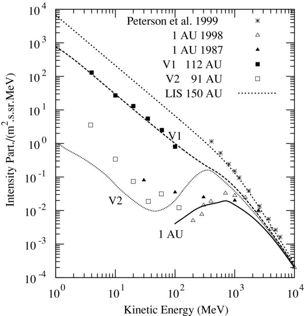
Figure 10. Same as the previous two figures, but with an asymmetric diffusion coefficient, such that at r > 90 AU, and for θ> 90° (i.e., the outer parts of the southern hemisphere), the diffusion coefficient at P< 300 MV does not have a kink as at other positions in the heliosphere. This produces an asymmetry in the calculated intensity such that the V2 spectra can be explained.
Download figure:
Standard image High-resolution image
Figure 11. Latitudinal dependence of the calculated intensities at 30 MeV and at 1, 91, and 112 AU for the spectra in Figure 10.
Download figure:
Standard image High-resolution image
The physical reason for this reduced low-rigidity diffusion coefficient in the southern regions of the heliosheath is unknown. It is suggested by the observed north–south asymmetries in various properties of the heliosheath, but as far as we can deduce, it is the only one that will produce a significant asymmetry in electron modulation, while leaving the modulation of nuclei largely unchanged. For clarity, we also note that this difference in low-rigidity diffusion coefficients is different from the one discussed in Dröge (2003) and references therein. In those papers, it is shown that at low energies electron and nuclei diffusion coefficients can differ significantly due to the particles' different response to a given turbulence spectrum. Here we hypothesize that the turbulence spectrum in the southern heliosheath may be different from that in the northern heliosheath, and that only low-energy electrons are sensitive to this difference—the nuclei are not, due to stronger energy loss effects.
4. SUMMARY AND CONCLUSION
The 2 to 160 MeV electrons that emerged above the background in the V1 detector in 2005 when the spacecraft was in the vicinity of the TS of the heliosphere, provide a new window to study the GCR modulation in the heliosphere. These electrons have low rigidities, in the range 2–160 MV, while GCR proton and most heavier nuclei studies are limited to rigidities P > 440 MV (proton kinetic energies T > 100 MeV) because at lower rigidities these species are submerged below their respective anomalous components.
It was shown that these V1 intensities can be understood in terms of standard modulation theory. The basic features are explained by an effective radial diffusion coefficient that increases with rigidity, P, above ≈300 MV, while becoming independent of P below that. Effects such as acceleration by the TS, latitudinal dependence of the modulation parameters leading to latitudinal transport, gradient, curvature, shock, and wavy neutral sheet drifts, as well as the size of the heliosheath all modify the amount of modulation moderately, but none of these parameters changes the nature of the explanation qualitatively.
A challenge of the observations has been that Voyager 2 has not seen similar increases since it crossed the TS in 2007 September, and the asymmetry between the V1 and V2 intensities was a factor of ∼10 in early 2010. At the same time, such asymmetries were not seen in the other species (although there are indications of a similar small, and possibly transient, asymmetry in 265 MeV n−1 He from 2009 onward). It was argued that this asymmetry is hard to explain as due to a radial effect (which may in principle be due to the fact that V1 is about 21 AU further out than V2), or to latitudinal asymmetries in the SW, drifts, or the size of the heliosheath. All of these will cause equivalent asymmetries in the intensities of nuclear species. We showed, however, that an asymmetry in the rigidity dependence of the diffusion coefficient at low rigidities provides a natural explanation for this effect: if at P< 300 MV the diffusion coefficient in the southern hemisphere is lower than in the northern hemisphere, then V2 will observe stronger modulation for (relativistic) electrons at T< 100 MeV than V1. This will hardly affect the (non-relativistic) nuclei, however, for two reasons. First, the adiabatic energy losses for the non-relativistic nuclei are much more severe than for the relativistic electrons, masking this low-energy dependence on the diffusion coefficient. Second, at P< 100 MV protons have kinetic energy T< 45 MeV, with heavier fully stripped nuclei (A/Z = 2) having T< 11.25 MeV n−1, and at these low energies these species are fully submerged below their respective anomalous components. The acceleration of these anomalous species is unaffected by the magnitude of the diffusion coefficients, as long as Vrs/κ>1. This condition is met for all low rigidities.
Thus, a stronger rigidity dependence of the diffusion coefficient at low rigidities in the southern regions of the outer heliosphere is sufficient to explain the low electron intensities observed by V2 in the heliosheath. Because nuclei at these energies are non-relativistic, this mechanism hardly affects the GCR and ACR nuclear species.
This work was supported by NSF grant ATM 0107181, the South African National Research Foundation, and PAPIIT-UNAM grant IN108409 in Mexico.