


ABSTRACT
In this paper, the third in a series of papers on topological changes of magnetic fields, we study how the dissipation of an initial current sheet (CS) in a closed three-dimensional (3D) field affects the field topology. The initial field is everywhere potential except at the location of the CS which is in macroscopic equilibrium under the condition of perfect conductivity. In the physical world of extremely high, but finite, conductivity, the CS dissipates and the field seeks a new equilibrium state in the form of an everywhere potential field since the initial field is everywhere untwisted. Our semi-analytical study indicates that the dissipation of the single initial CS must induce formation of additional CSs in extensive parts of the magnetic volume. The subsequent dissipation of these other sheets brings about topological changes by magnetic reconnection in order for the global field to become potential. In 2D fields, the magnetic reconnection due to the dissipation of a CS is limited to the magnetic vicinity of the dissipating sheet. Thus, the consequence of CS dissipation is physically and topologically quite different in 2D and 3D fields. A discussion of this result is given in general relation to the Parker theory of spontaneous CSs and heating in the solar corona and solar flares.
Export citation and abstract BibTeX RIS
1. INTRODUCTION
Under conditions of very high electrical conductivity, such as in the fully ionized, million-degree solar corona, the magnetic field is essentially frozen into the plasma and, therefore, the magnetic field topology cannot change. The topology is described by where each thin flux tube enters and leaves the volume and the twist and linkages of the magnetic flux tubes. Flux freezing prevents the mixing of local fluid volumes that trap different flux systems, resulting in thin sheets of intense electric current density flowing tangentially on magnetic flux surfaces. Through the thinning of these current sheets (CSs), the current density may be intensified to the point where resistive dissipation becomes significant. In this way, magnetic energy can be dissipated in spite of, or rather because of, the high electrical conductivity (Parker 1979, 1994, 2007). Solar flares are thought to release energy in a similar process (Tsuneta 1996; Shibata 1999; Aschwanden 2004).
In this third paper on topological changes, we continue our study of the spontaneous formation of CSs in topologically untwisted magnetic fields. These magnetic fields were introduced by Low (2006a), but their mathematical definition was first accomplished in the Appendix of Low & Janse (2009), hereafter referred to as Paper II. The magnetic fields in the solar atmosphere are generally twisted under that definition. The mathematics of spontaneous CSs is quite formidable for twisted fields but takes on a more tractable form for untwisted fields. Our series of papers exploits this tractability to make progress in understanding this important hydromagnetic process. In Janse & Low (2009), hereafter referred to as Paper I, we showed that a three-dimensional (3D) cylindrical potential field, as an example of an untwisted field, may have to form CSs when subject to a deformation of its volume that leaves its frozen-in field topology invariant. This result is basically similar to the one due to Hahm & Kulsrud (1985) showing CS formation in an initially force-free magnetic field as a result of an infinitesimal continuous deformation of its boundary wall.
In Paper II, we investigated this physical effect in the closing of the open part of an untwisted field in equilibrium external to a unit sphere. This open part of the field is associated with a global equilibrium CS built into the initial state. In that study, we addressed the question of how a new continuous equilibrium state can be reached following such a dynamical transition. The time-dependent dynamical problem is of course very complex, requiring sophisticated computational methods for a proper treatment. On the other hand, as we showed in Paper II, the following novel topological point can be made from a static analysis of this question. The dissipation of the initial CS is due to the reconnection of equal, finite amounts of opposite, open fluxes on the two sides of the sheet. Those closed flux systems not participating in the reconnection are left topologically unchanged because they are rigidly anchored to the boundary of the domain. In the frozen-in adjustments of these flux systems to arrive at the post-reconnection, global equilibrium state, each system undergoes a volume change so that CSs could form spontaneously within them in the manner described in Paper I. In contrast to the spherical model for a partially open field in an unbounded domain in Paper II, the study in the present paper treats a closed, untwisted, equilibrium field embedding an equilibrium CS in a Cartesian closed box. This model has implications for the magnetic topological changes associated with flares in the multipolar environment of a solar active region.
We refer the reader to Parker (1994) for a general review of the theory of spontaneous CSs. Although the untwisted fields are mathematically more tractable, our studies of these fields are far from complete, with various hydromagnetic properties still not fully understood, as we emphasized in Paper II. These ongoing studies are a step to treating the more complex processes involving twisted fields. We present the box model and the physical results in Sections 2 and 3, respectively. In Section 4, we give a general discussion of the Parker theory of spontaneous CSs that relates our series of three papers to that theory on general terms. This discussion also critically assesses the results of these papers in relation to some new concurrent developments on the Parker theory being published elsewhere, leading to a brief conclusion in Section 5.
2. MATHEMATICAL MODEL
We consider a pair of magnetostatic equilibrium states: the initial and the final state of a topologically untwisted field B in a simply connected domain, a Cartesian closed box of sides 2L. The initial and the final force-free field are subject to the given boundary-flux distributions:
That is, the magnetic field is closed, with some given flux distribution F(x, y), where ∫L−L∫L−LFdxdy = 0, at the bottom of the box, and no flux across the other sides. Unlike the first two papers in this series, we now study a closed magnetic field where the total magnetic volume is kept fixed. We set
This distribution of Bz on z = −L has three polarity reversal lines (PRLs), y = 0, and x = ±π/4, the first running perpendicular to and intersecting the other two. Instead of the higher order term cos3(2x), we could have used cos(2x) leading to the same three PRLs. Though a first-order term seems a more natural choice, using a higher order term has its mathematical advantages for the solution of the potential Φ1 as an infinite Fourier series, to be defined below. Analytical simplification contributes to retaining a high numerical accuracy helpful to the numerical computations in the study.
The initial state Bcs is everywhere potential except for a single CS in force balance, an acceptable equilibrium state under the condition of perfect conductivity. However, in the physical world of very high but finite conductivity, the CS will dissipate, the field reconnects, and eventually relaxes to an everywhere continuous equilibrium state. We believe that the field remains topologically untwisted, since the field deformations should not introduce any circulating fluxes into the field. This implies that the final state is the potential field Brmpot, as this is the only continuous, untwisted equilibrium state. By comparing the footpoint connectivity of the initial and final states, we get a glimpse into the dynamical transition from initial to final state. The essential point of the connectivity comparison is whether the difference in connectivity can be accounted for entirely by the reconnection due to the dissipation of the single, initial CS. We conjecture that for a non-trivially 3D field, the reconnection of the initial sheet cannot account for all the topological changes from the initial to the final potential state. Additional CSs would have to form, and only through the dissipation of these sheets can the field topology be changed to that of the potential field. This implies that CS formation in 3D fields is distinctly different from in 2D fields, where reconnection of a single sheet can account for all the topological change. Our semi-analytical model depends crucially on the stipulation that the end state is potential for the physical and topological reasons given. The issues surrounding this stipulation are interesting but not simple. We return to discuss this point in Section 4.
The construction of the initial state Bcs is rather involved. In order to see its mathematical relationship with the final potential state, we begin our study by first determining the latter by solving for Bpot = ∇Φpot subject to the boundary conditions (1)–(6). From the solenoidal condition (17)

Solving this Laplace equation subject to the boundary conditions, we find
To derive an analytical solution for the initial state Bcs containing a CS subject to boundary conditions (1)–(6), we use the method of Zhang & Low (2001). This method requires several auxiliary potential fields to express Bcs explicitly.
We start by modifying boundary condition (6) to the form
reversing the sign of the original boundary values of Bz on the side of the PRL x = −π/4 to the nearest vertical boundary at x = −π/2. We then solve for the potential field Bm = ∇Φm subject to the modified boundary conditions. This requires two steps.
We introduce the potential field B1 = ∇Φ1 subject to the given boundary-flux distribution:
Direct solution of the Laplace equation gives
where  and
and  , and the constant coefficients a2n + 1 and b2n are
complemented by  for n = 1 and
  for n = 3. Then, the magnetic field Bm we seek is given by

The potential fields Bpot and Bm differ through their respective boundary conditions, one set being modified from the other by a reversal of the sign of Bz on z = −L in the strip −π/2 < x < −π/4. In this strip, two regions of opposite polarities are separated by the PRL y = 0. The field Bpot contains lines of force (LOFs) that connect all the different polarity regions on z = −L. In particular, there are LOFs connecting the two bipolar regions in the strip −π/2 < x < −π/4 on z = −L to other regions on z = −L. By the nature of the modification of the boundary conditions, the LOFs of Bm are such that these two bipolar regions are not magnetically connected with the other parts of z = −L. The flux that connects them is magnetically isolated from the rest of the field by a flux surface S that intersects z = −L along x = −π/4 and divides the box domain into two subdomains, which we denote by V1, containing the isolated flux system, and V2, the complementary subdomain. Note that Bm is everywhere continuous. By the definition of a flux surface, Bm is tangential along S. These properties allow us to define the following initial state containing a CS:
that is, we reverse the sign of Bm in the region V1. This step reverses the field vector of Bm on the V1 side of flux surface S, transforming this surface into a CS. The reversal leaves |B2cs| continuous across S, satisfying force balance for the equilibrium of this surface. So, the initial field is in macroscopic equilibrium under the condition of perfect conductivity, everywhere potential except at S. The volumetric reversal of sign also reverses the polarity of the strip −π/2 < x < −π/4 on z = −L back to the polarity in the original boundary condition. Hence, Bcs and Bpot satisfy the same boundary conditions (1)–(6). The resistive dissipation of the CS S in Bcs could then proceed with no change in the boundary conditions to arrive at Bpot as the final state.
3. RESULTS
We study two topologically untwisted force-free fields: an initial state containing a CS and the corresponding final state which does not contain any CSs. As previously reasoned, we take this final state to be the potential state. We compare the footpoint connectivities of the initial and the potential state to determine whether the field can reach the potential state solely through the dissipation of the initial CS.
Before we compare the footpoint connectivity, let us first take a closer look at the initial and the potential state. Figure 1 shows several LOFs of the initial field. In addition, at the bottom of the box, z = −L, contours of Bz are drawn. The solid (dashed) contours represent negative (positive) Bz, and the solid straight lines, dividing the bottom of the box into six regions, are the PRLs along which Bz = 0. The direction of the LOFs can be inferred from the signs of Bz at their respective footpoints. The CS, on a flux surface S, is dividing the box into two subvolumes, which can be identified in Figure 1 in terms of the intersection curve between S and the boundary walls of the box. The intersection of S with the bottom of the box is just the line x = −π/4 bounding the bipolar region −π/2 < x < −π/4 on z = −L. The two almost coincident, dashed LOFs have footpoints on opposite sides of the line x = −π/4 on z = −L, chosen just inside the domain. These two LOFs sandwich S between them, indicating where S intersects the two vertical walls and the top wall of the box. By its construction, the LOFs on the immediate opposite sides of S are tangential to S but of opposite signs, accounting for the discrete current flowing along S. With no LOFs crossing S, this flux surface isolates the bipolar flux system occupying the subvolume V1 to its left side. The LOFs of this system straddle the single PRL y = 0. There are no magnetic neutral points, i.e., points where |B| = 0, in this isolated bipolar flux system. In contrast, the LOFs in the multipolar flux system in the subvolume V2 to the right of S connect over the two intersecting PRLs, the y = 0 and x = π/4 lines. Magnetic neutral points and their separatrix flux surfaces occur naturally in this flux system. To avoid cluttering the figure, we show the separatrix surfaces in Figure 3 in terms of black dashed lines marking the intersection of these surfaces with the bottom of the box z = −L. We will later return to discuss these separatrix surfaces together with those belonging to the final potential state.
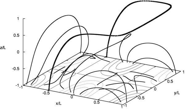
Figure 1. Eighteen solid lines and the two dashed lines represent LOFs of the initial field, associated with Equation (15). The black curves at the bottom of the box, z/L = −1, are the contours of Bz with solid curves representing Bz ⩾ 0 and dashed curves representing Bz < 0 and the parameter L = π/2. The initial field contains a current sheet, which is a surface whose boundary comprises the thick curve shown and the x/L = −0.5 line on the bottom of the box. This thick curve is identified by drawing two very closely separated dashed LOFs on the two sides of the current-sheet surface. Note that this curved sheet separates the box into two subvolumes, a bipolar region on the left-hand side, V1, and a multipolar region on the right-hand side, V2.
Download figure:
Standard image High-resolution imageFigure 2 shows several LOFs of the final potential field. The solid lines have the same starting footpoint as the corresponding solid lines in Figure 1. The dashed LOFs have been added to illustrate the symmetric nature of the potential field. That is, the field is symmetric about the y-axis and symmetric about the x = −π/4 plane in the region x < 0 and about the x = π/4 plane in the x > 0 region. Furthermore, the field is symmetric about the x-axis, but as the LOFs originally were chosen to illustrate the field configuration of the initial field and not the potential field, this property is not well captured by Figure 2. With the CS surface S of the initial field removed, the original isolated bipolar flux to the left side of S is now reconnected with the other flux system to give the potential field with its own unique set of neutral points and separatrix surfaces. These separatrix surfaces are shown in Figure 3 in terms of the red dashed curves marking their intersections with the base z = −L. The field symmetry about the x-axis is clearly illustrated by these separatrix footprints. In contrast to the potential field, the initial field is only symmetric about the y-axis, as the CS breaks the symmetry in the x-direction.

Figure 2. LOFs of the potential field, described in the text (Equation (8)). The 18 solid lines have the same starting footpoint as the solid lines in Figure 1, however, the ending footpoints may differ. These 18 LOFs were chosen to illustrate the initial field and do not well capture the symmetric nature of the potential field. Therefore, some additional LOFs (dashed lines) have been added. The black curves at the bottom of the box, z/L = −1, are the contours of Bz with solid curves representing Bz ⩾ 0 and dashed curves representing Bz < 0 and the parameter L = π/2.
Download figure:
Standard image High-resolution image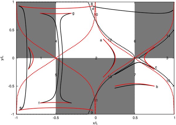
Figure 3. Comparison of the footpoint connectivity at the bottom of the box, z/L = −1, for the initial and the potential field. The parameter L = π/2, the black (red) dashed curves are the separatrix footprints of the initial (potential) field, and the black (red) solid lines are LOFs of the initial (potential) field. The starting footpoints are the same for both fields, however only certain LOF-pairs also have common ending footpoints, e.g., the pair labeled a. The LOF-pairs with different ending footpoints either terminate in different topological regions, illustrated by the LOF-pairs c, d, e, f, and g, or they terminate at different locations within the same topological region, e.g., the LOF-pair b.
Download figure:
Standard image High-resolution image
In Figure 3, we compare the footpoint connectivity of the initial and the potential field, here focusing on eight of the LOFs shown in Figures 1 and 2. Note again that these LOFs have common starting footpoints in the initial and the potential field. The white and gray squares indicate where Bz ∣ z = −L is positive and negative, respectively. The solid black (red) lines represent the LOFs of the initial (potential) field and the dashed black (red) curves represent the separatrix footprints of the initial (potential) field. The separatrices divide the initial field into four topologically distinct regions, while the potential field consists of seven topological regions.
Taking both sets of separatrix footprints into account, we divide the box into 15 regions, which are numbered in Figure 3. Let us quickly go through the footpoint connectivity in these regions before we discuss these results in more detail. In regions 1–3, all LOFs straddle the y-axis, and in these regions the initial and the potential field footpoint connectivities are identical, e.g., see the LOF-pair a, which is a pair of LOFs picked from the initial and potential fields sharing a common starting footpoint. In the remaining regions, the footpoint connectivities of the two fields differ. In regions 4 and 5, the initial LOFs span across the y-axis, while the potential LOFs connect across the x = −π/4 line, as seen in LOF-pairs e, f, and g. In regions 6 and 7, all the initial and the potential LOFs connect across the x = π/4 line. Although both fields connect to the same topological region, we note that the LOF-pairs, e.g., the LOF-pair b, have different ending footpoints. In regions 8 and 9, none of the LOFs straddle the y-axis. The initial LOFs have corresponding footpoints far right in the box, and the corresponding footpoints of the potential field are located far left in the box, as seen in the LOF-pair d. In the two smallest regions, regions 10 and 11, the initial LOFs cross the x = π/4 line, while the potential LOFs cross the y-axis. In regions 12 and 13 (14 and 15), the initial LOFs straddle the y-axis (x = π/4 line), while the potential LOFs cross the x = π/4 line (y-axis).
We find that the reconnection of the initial CS cannot account for all the topological changes from the initial to the final potential state. The dissipation of the initial sheet only changes the connectivity in the vicinity of the sheet. In the remaining regions, the connectivity is unaffected by the initial dissipation. In most of these "unaffected" regions, the initial field connectivity does not match the potential field connectivity; see regions 6–15 in Figure 3. Hence, after the initial CS has dissipated, the field cannot evolve, under the frozen-in condition, into the potential state. This is exemplified by the LOF-pair b, which has different ending footpoints within the same topological region; the LOF-pair c, which has ending footpoints in different topological regions; as well as by the LOF-pairs d and e, where the initial LOFs are not able to reconnect to become the potential LOFs d and e, in sharp contrast to the initial LOFs f and g which reconnect to become the potential LOFs f and g.
We believe additional CS formation and dissipation will pervade parts of the field, in order to change the "mismatched" footpoints in regions 6–15. First, after several reconnection events, either sequential or simultaneous, the potential LOF configuration can be attained. In regions 1–5, additional CS formation is not needed. In regions 4 and 5, the dissipation of the initial CS fully accounts for the topological changes, while in regions 1–3, the initial and potential fields share a common footpoint connectivity. (The lack of additional CS formation in regions 2 and 3 is thought to be due to the field symmetry about the y-axis. As seen in Paper I and Paper II, symmetry limits/prevents sheets from forming.)
During the transition from the initial to the potential state, the field undergoes large changes. As we have seen from the footpoint connectivities, additional CSs should form in most, but not all, regions. Furthermore, both the number of topological regions, as well as the volume of these regions, change. The initial field has four topological regions, a "left region" built up of regions 1, 2, 4, 5, 12, and 13, an "upper region" containing regions 6, 8, 10, and 14, a "lower region" (regions 7, 9, 11, and 15), and a "right region," which is just region 3. The potential field has seven topological regions, a "left region" which is just region 1, a "mid region" (regions 2, 10, and 11), a "right region" (regions 3, 14, and 15), an "upper left region" (regions 4 and 8), a "lower left region" (regions 5 and 9), an "upper right region" (regions 6 and 12), and a "lower right region" (regions 7 and 13). Since most of the initial and potential topological regions do not overlap, it is difficult to compare the volume of these regions. However, there is one region that undergoes a simple expansion: "the right region", where the potential state region encapsulates the initial state region. As the initial CSs dissipate, the energy density and the isotropic pressure in the vicinity of the sheet decrease, causing a local implosion as the surroundings, with their now superior pressure, expand (Hudson 2000; Janse & Low 2007). This effect is more clearly seen in Paper II. There the initial and potential fields have only three topologically distinct regions: two polar regions and an equatorial region initially containing a CS. After the CS has dissipated, the equatorial region contracts and the polar regions expand.
Finally, we draw attention to the short, straight, black dashed line that lies right on the PRL y = 0 separating the bipolar region to the right of x = π/4 in Figure 3. This short line on the z = −L base of the box is actually by itself a degenerate separatrix "surface" of the initial field. There is a set of LOFs of the initial field belonging to region 2 with the following property: these LOFs arch over the PRL y = 0 but are shaped in 3D space like the letter M. Each LOF rises from its footpoint at the base where Bz > 0 into the region x > π/4 then dips down and tangentially graze the base z = −L at a point on the short straight dashed line coinciding with y = 0. This LOF continues beyond that grazing point by rising back into the box to complete its other half of the M-shaped configuration. In doing so, the LOF returns to the space x < π/4 before finding its second Bz < 0 footpoint on z = −L. Since the field is symmetric in the box about the plane y = 0, the M-shaped LOF is similarly symmetric, which means that it grazes across the PRL y = 0 at right angle.
Such M-shaped LOFs associated with multipolar flux systems were investigated in 2D as a natural site for CS formation without involving the presence of a neutral point (Aly 1987; Low 1987; Moffatt 1987; Low & Wolfson 1988). A non-trivial extension of this field topology to 3D referred to as a magnetic bald patch was discovered by Titov & Demoulin (1999) as a natural feature of magnetic flux ropes; see also Demoulin et al. (1996), Low & Berger (2003), Demoulin (2007), and Schmieder et al. (2007). Returning to Figure 3, the propensity for a CS to form at the grazing point of the M-shaped LOFs is physically easy to understand, as explained in these works. The grazing point, as the bottom of the M-dip, can readily lift upward during a frozen-in adjustment of the field in search of the nearest equilibrium state available. This results in a field reversal layer below it that would then collapse into a CS extending from the rising M-dip to the boundary below where other LOFs are rigidly anchored.
To understand why this M-dip would rise from the base z = −L during the transition from the initial to final potential states, we take note of the shape of the CS surface S in Figure 1. This shape indicates that the equilibrium of the initial state is characterized by the bipolar flux occupying V1 to the left of S being dominant in the upper parts of the box. In other words, equilibrium is maintained by this bipolar flux pushing at S in the upper reaches into the multipolar flux system in V2 on the right side of S. When the CS S dissipates, the field relaxes via a contraction of the bipolar flux as it loses its bipolar topology by reconnection with the other flux system across the CS surface. Correspondingly, this other flux system expands upward with the consequence that the M-shaped LOFs lift their M-dips upward from the base of the box.
It is well known that CSs naturally form at magnetic neutral points (Sweet 1969; Syrovatskii 1981). The formation of CSs at bald patches is a similar frozen-in effect arising from a rigid boundary interacting with a locally tangential magnetic field. The field in our model is multipolar and both effects are involved in its transition from the initial to final states.
4. GENERAL PHYSICAL ISSUES
The box model we have studied and the spherical model of Paper II illustrate the same basic hydromagnetic effect in two contrasting 3D magnetic geometries. This effect is inferred from several basic properties that are understood to varying degrees of certainty. Here, these properties are discussed to identify several unresolved fundamental issues and to address a few others that can be resolved. We begin with a statement of the Parker (1994) theory in the most general terms and relating it to the box model that narrowly deals with untwisted fields.
4.1. The Parker Theory
With the tenuous corona in mind, we henceforth take a field B in equilibrium to be force-free, described by the equations


neglecting all other fluid forces. This field has a field-aligned current density given by

where α is a scalar function of space, constant along each LOF. This property is expressed by

which follows from Equations (17) and (18).
When not in equilibrium, the field evolves according to the induction equation
where v is the velocity of the perfectly conducting fluid. This equation is coupled to the other hydromagnetic equations that are not needed for our purpose here. By the induction equation, a field anchored rigidly at the boundary of the box domain has a fixed normal field component Bn|S, S denoting the boundary. The field also preserves its topology T during evolution. At any instant of time, the ordinary differential equations (ODEs)
can be solved for the LOFs. Under the frozen-in condition, the LOFs are fluid lines deforming continuously at some (continuous) velocity v. Topology T is taken in its textbook definition to mean the properties of these fluid lines that are definable independent of geometric metric and invariant under arbitrary continuous deformation.
Since a given field is identified with a prescribed pair (Bn|S, T), fixed for all time, it follows that its force-free state defined by Equations (16) and (17) is subject to the prescribed pair (Bn|S, T). This is a general statement of the magnetostatic problem posed by Parker (1972). The Parker (1994) theory states that for most prescribed T, this magnetostatic problem does not admit analytic or continuous solutions.
To pose the Parker problem in general terms for the box model, first note that the flux enters and leaves the box through the base z = 0. By its global nature the field topology is naturally expressed by integral equations. The LOFs define a map of the base z = 0 of the box onto itself to identify the pairs of magnetic footpoints of the LOFs. This map, invariant under the frozen-in condition, is expressed by the footpoint-to-footpoint integrals of the ODEs (21) along the LOFs. Other integral equations express the interweavings among two or more LOFs. Therefore, the Parker problem is a boundary value problem posed by a nonlinear system coupling such integral equations, as many as required to fully specify T, to the force-free partial differential equations (PDEs). This is an overdetermined system that may not have analytic solutions, a property suggested by its mathematical structure but extremely difficult to prove or demonstrate. We refer the reader to Janse et al. (2010) for a detailed analysis of that system of integro-PDEs.
Analyticity is too strong a mathematical condition for most prescribed T to be compatible with the point-by-point force-free condition, because of a diverse variety of physical reasons analyzed by Parker (1986a, 1986b, 1994); see also Low (1990) and Ng & Bhattacharjee (1998). Under the frozen-in condition, the force-free field as a minimum-energy state always exists and preserving T can never be compromised. Physics avoids the incompatibility between the two demands by relinquishing analyticity for the weak solutions to the Parker problem (Courant & Hilbert 1962). These are solutions containing surfaces of tangential discontinuities in B subject to two requirements. For these surfaces to be in macroscopic force balance, the magnetic pressure B2 must be continuous across them, satisfying the integral version of the force-free PDEs. In addition, the CSs in these surfaces and the current density in the continuous parts of the field, together under Ampere's law, define a global field that has exactly the invariant topology T.
Let us be specific about the central point of the Parker theory that most of the topologies a field may possess in a given physical system are not compatible with an analytical force-free state. Consider the box model with a fixed Bn|S. Denote by Tall the set of the topologies of all the continuous fields, not necessarily in equilibrium, admissible in the box. We also have the set Tfff of topologies of the analytic force-free fields admissible in the box. For 3D fields, these are typically infinite sets. Then, in general, Tfff is a subset of Tall of measure zero, meaning that as infinite sets Tfff is negligibly small compared to Tall. A useful analogy is the sparse scattering of the infinitely many rational numbers on the real line among the irrational numbers, the latter also infinitely many but at a higher order of infinity.
The physical significance of this point is that the arbitrary pick of a topology T has zero probability of T ∈ Tfff. In other words, a naturally occurring astrophysical field is extremely unlikely to have a topology belonging to Tfff. The box model illustrates a particular consequence of this implication in Sections 2 and 3. Following the resistive dissipation of the built-in CS in the initial state, the reconnected field has a topology T ∉ Tfff. This is the general expectation of the Parker theory for all reconnections in 3D fields, whether the field is twisted or not. The topology of a reconnected field depends sensitively on the nature and details of reconnection and the chance of the reconnected topology being in Tfff is effectively nil.
To lend further specificity to this point, let the fluid be extremely highly conducting but viscous. The anchored field in the box must then evolve to a minimum-energy state preserving its topology T so long as thin CSs have not yet formed in a phase of its evolution when the frozen-in condition is approximately valid. During this phase, the free energy of the field is transformed into kinetic energy that is irreversibly removed by viscosity. With T ∉ Tfff, CS formation is inevitable and the CSs thin down toward zero thicknesses until the frozen-in condition breaks down, whereupon reconnection sets in and creates a new topology T'. The chance of T' ∈ Tfff is negligible. Thus, the reconnected field is expected to be driven to form new CSs and the process then repeats.
In this physical picture, once CSs have formed in a highly conducting plasma, taking the box model to keep ideas specific, they would just keep forming by the above probabilistic argument. This interesting physical possibility is extremely intractable to prove mathematically or to demonstrate with 3D numerical simulation. The field in the box in Section 2 demonstrates a limited case of it, namely, in the context of topologically untwisted fields. This model starts with a large CS in equilibrium and a finite amount of free energy. If we accept the model result, then the field must keep changing its field topology until it becomes the unique potential field Bpot with topology Tpot. It is, in principle, possible for the reconnecting field to fortuitously arrive at the topology Tpot at some instance in time, beyond which the field may evolve to the terminal state Bpot with no need for further CS formation and dissipation. But, generally, we expect the terminal state Bpot to be approached only asymptotically, with CS formation and dissipation continuing to change the field topology toward Tpot. As the free energy of the field runs out, the reconnections are energetically weak and negligible in this asymptotic approach to the potential state. This is the restless nature of a field in a highly conducting fluid (Parker 1979, 1994, 2007).
4.2. Twisted and Untwisted Fields
To see our concept of a topologically untwisted field in a broader context, consider the first and simplest demonstration of the Parker theory applied to the uniform field  in the unbounded domain anchored at the two plate boundaries z = ±L, where L is a constant (Parker 1972). Momentarily relax the rigid anchoring field in order to employ some arbitrary, continuous footpoint displacements that deform the uniform field into a some nonequilibrium state B1 with topology T1. Now restore the rigid anchoring. The topology T1 is permanently locked into the deformed field under the frozen-in condition. The distributions of B1,z at z = ±L, not necessarily uniform, are now also fixed. The Parker problem then demands for a force-free state for B1 subject to (B1,z|z = ±L, T1) treated as arbitrarily given. By taking the amplitude
  of the footpoint displacements, small compared to the plate separation 2L, a perturbational analysis may be used. Denote the desired force-free state by B = B0 + δB. Then if δB is analytic, it can be expressed as an infinite series in , subject to the caution on such a usage expressed by Rosner & Knobloch (1982). Another important parameter of the displacements is their characteristic (horizontal) scale l. Parker (1972) showed that if analyticity of δB is assumed, the force-free equations alone require δB to be independent of z in the limit of l ≪ L. Footpoint displacements can be prescribed that trap uncorrelated sequences of interlocking braids of the LOFs along the flow of the deformed field from one plate boundary to the other. Such a topology is inconsistent with a z-independent field. Hence, the conclusion follows that most footpoint displacements would create a T1 that renders the deformed field without an analytic force-free state.
Several authors took the demand of z-independence out of the restriction l ≪ L adopted by the Parker demonstration and had incorrectly equated the Parker theory with the completely unqualified claim that there can be no z-dependent equilibrium states in −L < z < L. Based on such a misunderstanding of the theory, z-dependent magnetostatic solutions had been published as counterexamples to the Parker theory (Bogoyavlenskij 2000a, 2000b; Craig & Sneyd 2005); see the responses to these works by Parker (2000) and Low (2010a). The unqualified claim is obviously false and has nothing to do with the Parker theory. In the finite-l regime, magnetostatic solutions must vary with z. Such z-dependent solutions were known well before these objections were published; see van Ballegooijen (1985) and Zweibel & Li (1987). The complete set of explicit solutions of Zweibel & Li (1987) shows that if the horizontal scales of B1,z|z = ±L are taken to be vanishingly small, the variation of the field with z in the main interior also becomes vanishingly small, consistent with the demonstration of Parker (1972). It was realized only recently that the simplest of these z-dependent solutions are the potential fields matching any prescribed B1,z|z = ±L (Low 2010a), showing that there is nothing of interest in the unqualified claim extraneously introduced by Bogoyavlenskij (2000a) and Craig & Sneyd (2005). We refer to Low (2010a) and Appendix B in Janse et al. (2010) for detailed analyses of this misunderstanding of the Parker theory.
The Parker two-plate demonstration has been extended to finite l (Low 2010b). For a small enough l, the variations of analytic force-free fields with z can be separated into two types, one reflecting the force-free condition in the domain interior and the other as boundary layers of thicknesses comparable to l. The latter relates the interior variation to the boundary conditions at z = ±L. Of course this separation disappears for l comparable to or larger than 2L. This new demonstration recovers a version of the results on the topologically untwisted fields in Paper I and Low (2007) and it is interesting to relate the different versions.
First, consider the two-plate problem treated by Low (2010b). Keep the footpoints at z = −L fixed and displace the footpoints at z = L. The general footpoint displacement is a linear superposition of an incompressible-rotational component with a compressible-irrotational component. By admitting strictly compressible-irrotational displacements, we create in each case an untwisted (nonequilibrium) field out of the initial uniform field. Let us denote this field and its topology by B*1 and T*1, respectively, with the asterisk indicating its untwisted nature. The normal field component B1,z remains uniform on z = −L but is no longer uniform on z = L. The interesting point about this construction is that an infinity of compressible-irrotational displacements exists to take the uniform field into a continuum of fields of this kind, all sharing the same B1,z|z = ±L but possessing different LOF connectivities between the two plates. That is to say, these fields are not deformable into one another under the frozen-in condition. Denote the set of topologies of these untwisted fields by T* ⊂ Tall, the latter being the set of all admissible topologies.
To summarize, all continuous fields B1 deformable from the initial uniform field sharing a common B1,z|z = ±L can be separated into topologically twisted and untwisted fields. The untwisted fields B*1 have topologies T*1 ∈ T* ⊂ Tall, whereas all the other fields with topologies in the subset complement to T* are twisted, by the fact that they are created by rotational footpoint displacements. In particular, the potential field Bpot, defined uniquely by the fixed B1,z|z = ±L, is untwisted, with a topology Tpot ∈ T*. Of course, we also have Tpot ∈ Tfff, the latter containing the topologies realized in the analytic force-free fields. Each of these analytic fields can be expressed as an infinite series in , the small amplitude of the footpoint displacement. If the footpoint displacement creating a particular force-free field is irrotational, then substituting its infinite series into the force-free equations leads to the conclusion that the field must be the unique potential field Bpot. This means that there is only one element in common to the set Tfff and the set T* of untwisted topologies created by irrotational footpoint displacements. It follows that those deformed fields B*1 with topology T*1 ≠ Tpot from the set T* must find force-free states containing CSs.
Paper I presented a similar result for the fields in an upright cylindrical domain. With a fixed boundary-flux distribution, this domain admits an infinity of nonequilibrium fields with topologically untwisted T* making up a set T* using a correspondingly similar notation. The unique potential field Bpot is among these fields with topology Tpot ∈ T*. The claim is then argued for Tfff∩T* being a set of just one element, namely, Tpot. The arguments are not mathematically rigorous, as discussed in Paper II. The similar result in the finite-l demonstration of the Parker theory is mathematically rigorous within the framework of the -series, but cannot be carried over to the cylindrical fields because the untwisted fields in the two studies are not defined the same way.
Let us examine the untwisted field in the box in the sense of Paper I. Express a general field in the Chandrasekhar–Kendall (CK) representation:
in terms of two generating functions (ψ, ϕ). We use this representation as described in Appendix A of Paper I that decomposes any given B into a unique pair (Bψ, Bϕ). This use is distinct from the original use by Chandrasekhar & Kendall (1957). Take any flux tube of B and consider its cross section σ with a closed boundary ∂σ on a constant-z plane. The field Bψ alone accounts for the net flux of B across σ. The field Bϕ, lying on the z-plane, accounts for the circulation C(∂σ) of B along the closed boundary ∂σ. Any field in an arbitrary state has a CK representation with both (Bψ, Bϕ) generally not zero. The topologically untwisted fields are defined to be those continuously deformable into a state with Bϕ ≡ 0. In such a state, the passage of the flux of B across every constant-z plane is characterized by C(∂σ) = 0 for every flux tube. The italic emphasis is essential. The geometric twist of LOFs on the tube boundary around a flux tube says nothing about similar twists within the tube. But if every definable tube shows no LOF circulating on its tube boundary, then we have an intuitive meaning for the field being topologically untwisted. The qualifier "topological" refers to the fact that such a field, even if presented in an incidental state of complex contortion, can always be deformed into a Bϕ ≡ 0 state.
Our studies are restricted to simply connected domains, a qualification obvious but not explicitly stated in Papers I and II; see the criticism of Huang et al. (2009) and the response of Janse et al. (2010). By simply connected is meant that all closed curves in a domain can be continuously contracted to a point. In contrast, a multiply connected domain has one or more "holes" punctured right through it, exemplified by the torus as a doubly connected domain. In that domain, closed curves that do and do not encircle the hole of the torus constitute two classes, those that cannot and can, respectively, be contracted to a point. A potential field in a simply connected domain such as the box or the cylinder is uniquely defined by the boundary-flux distribution Bn|S and is untwisted as defined above using the CK representation. In contrast, a prescribed Bn|S defines an infinity of potential fields in a multiply connected domain, all except one containing twist as indicated by nonzero magnetic circulations along closed curves not contractible to a point. These circulations present no contradiction with the potential state of the field. The implied net current across the area bounded by the nonzero-circulation closed curve can exist in the hole that the curve encircles. The exceptional, untwisted field among the infinite set of potential fields is the one with no current passing through the holes of the multiply connected domain. We refer the reader to Janse et al. (2010) for a more complete analysis.
Aly & Amari (2010) question the concept of the topologically untwisted field in Paper I with a fundamentally interesting point. It is common practice to regard an anchored field to be twisted if it has nonzero relative helicity (Berger & Field 1984). This helicity is an integral over the field domain, measuring the twist relative to the unique potential field defined by the prescribed Bn|S. By the nature of its construction, this integral is more accurately described to be a measure of the difference in topology between a given field and its reference potential field. As an integral, it is a crude measure in the sense that when the relative helicity is zero, it does not mean that the given field is topologically deformable into the potential field. A twisted field can easily be constructed with zero relative helicity to make this point. It is a powerful tool when the relative helicity is not zero, for then the conservation of the relative helicity in the fixed domain implies that the given field is not topologically deformable into the potential field.
Now consider the topologically untwisted cylindrical fields of Paper I, reminding ourselves that we are restricted to a simply connected domain. All the untwisted topologies in the infinite set T* are distinct, among which is Tpot, the topology of the unique potential field. Aly & Amari (2010) showed that the relative helicities of the explicit untwisted fields in Paper I, with the exception of the potential field, are nonzero. They correctly pointed out that these fields are twisted by the common interpretation of the relative helicity. What seems clear is that the concept of twisted and untwisted fields needs to be eventually redefined. If the concept of relative helicity is reviewed from first principle, the nonzero relative helicities calculated by Aly & Amari may be stated minimally to be showing that these fields, including the reference potential field, are all topologically distinct. This difference in topology is also indicated by their different LOF connectivities shown in Paper I. This fundamental issue has recently been resolved by the construction of absolute helicities applicable to anchored and unanchored fields alike (Low 2006b; B. C. Low 2010, unpublished). We defer further discussion of the relative helicities of the untwisted fields in Paper I to B. C. Low (2010, unpublished) where an absolute helicity for the cylindrical fields is constructed without involving the potential field.
Returning to the simply connected box model, if we accept the claim that Tfff ∩ T* contains just Tpot, then any untwisted field B*1, with T*1 ≠ Tpot, must keep forming CSs and change topology by reconnection to finally arrive at the potential state. The argument leading to the claim is complicated by the interplay between the writhe and twist of an anchored flux tube, pointed out to us by E. N. Parker (2009, private communication) and an anonymous referee. Let us briefly address this criticism to understand a basic issue implied.
4.3. Flux Tube Writhe and Twist
Select a cylindrical flux tube of the rigidly anchored uniform field in the two-plate problem. Continuously push its surrounding fluid and field aside to deform the tube into a form that is helical around an external (vertical) axis perpendicular to z = ±L. The two tube footprints, one located directly above the other, are fixed on z = ±L, and no intrinsic net twist has been imparted to the flux tube. Therefore, as the LOFs of the deformed tube make their helical paths around the external vertical axis in one handedness, they must twist about one another in the opposite handedness in order to find their respective second footpoints fixed on the second boundary. In other words, by deforming or writhing the anchored flux tube into a helical shape, its LOFs not only take up that helical shape but do so with a twist of the opposite handedness within the deformed tube. This topological property is easy to demonstrate qualitatively with explicit examples, but has been expressed quantitatively only recently (Berger & Prior 2006).
The preceding exercise suggests the possibility that flux-tube writhing may arise and survive during the relaxation of a topologically untwisted field to a force-free state. That state is then characterized with α ≠ 0 in apparent contradiction to the claim that Tfff∩T* contains just Tpot. This possibility a priori does not disprove but does question the claim. To rigorously establish this claim requires directly solving the Parker magnetostatic problem to eliminate that possibility for all topologically untwisted fields, a formidable undertaking. It is thus useful to know that this elimination is possible in B. C. Low's (2010, unpublished) finite-l demonstration of the Parker theory. The ordering of terms in ascending powers of in the series solutions for the analytical force-free states allows for the separation of the twisted from the untwisted fields without being complicated by the writhe-twist interplay.
There are two subtle points worthy of mention to see the basic issue clearly. Any field can have any one of its flux tubes writhed to create LOF twist, such as we have demonstrated above with the uniform field. Such a creation of twist by itself has no significance for whether a force-free state with α ≠ 0 is available to a given field. A force-free state is a minimum-energy state subject to a fixed (Bn|S, T). Nonequilibrium fields sharing this same pair of invariants, in small departures from that force-free state, can be continuously deformed into it along an evolutionary path of monotonically decreasing energies. Therefore, only those writhings that decrease the energy of a nonequilibrium field are of interest to the question of whether an available force-free state may have α ≠ 0. Increasing the writhe of a flux tube increases the field energy because the flux tube has lengthened and pushed into its surrounding field. Such an evolution is not one directed toward a minimum-energy state.
The second point becomes relevant when we realize that, even if an energy-decreasing evolution favors a topologically untwisted field to develop writhes and twists, the whole question of the general incompatibility between the preserved topology T and equilibrium at all points in space, raised by the Parker theory, remains. That is, despite the possibility for the field to be energetically favored to evolve into an α ≠ 0 force-free state, it is a separate question whether that state is analytic. This discussion shows that there is much interesting physics to explore in this magnetostatic problem.
5. CONCLUSION
In this series of papers, we step outside of the formidable twisted magnetic fields to understand the basic physics of the Parker theory in terms of the simpler untwisted fields. We have generalized the potential fields to the larger class of topologically untwisted fields, defined by their common property of each being deformable from any one of its admissible states, under the frozen-in condition, into a ϕ ≡ 0 state in an appropriate CK representation. We emphasize again that our studies are restricted to simply connected domains. We refer the reader to Janse et al. (2010) for a fresh overview of the Parker theory where the implications of domain connectivity and shapes are discussed. That overview (their Appendix B) also identifies and analyzes a published misunderstanding of the Parker theory that has unfortunately propagated into the literature.
Our definition of untwisted fields based on the CK representation lacks generality because this representation is not available for domains of arbitrary shapes. Nevertheless, our definition of untwisted fields is unambiguous in our study. They provide insights into the Parker theory and their study leads us to the novel topological and physical questions fundamental to understanding CS heating in the corona, as discussed in Section 4.
The principal point of the Parker theory is that, for a 3D system, the infinite subset Tfff is of zero measure compared to the set Tall of all admissible topologies. When a CS dissipates resistively via reconnection of the field, the chance of the reconnected topology of the field happening to belong to Tfff is practically zero. Once CSs get to form in a fluid with an extremely high but finite conductivity, their dissipation must lead to repeated further CS formation. The probabilistic unlikelihood remains unchanged for the field to acquire a topology belonging to Tfff. Yet the field does eventually find a terminal analytic minimum-energy force-free state. The reason has to do with the availability of free energy. As free energy runs out, the field approaches one of these analytical end states asymptotically, with CSs forming at decreasingly weak intensities. The above general behavior is suggested by the topologically untwisted fields in the box model in Sections 2 and 3, for which the Parker problem takes a form more tractable than that for twisted fields.
CS formation in the box model comes in two forms. The frozen-in fluid–field interaction around a magnetic neutral point can readily create CSs along the separatrix flux surfaces of the neutral point. The fluid volumes on the two sides of a separatrix flux surface naturally slip over each other discontinuously for the system to seek a lowering of magnetic energy. CS formation associated with neutral points operates the same way in 2D systems and is the only type of CS formation possible in those systems. In 3D systems, the additional degree of freedom for fluid motions allows any flux surface to become a CS by the same basic discontinuous slipping of fluids along the two sides of that surface. This 3D feature is basic to the Parker theory and is the most interesting aspect of the box model. Subsystems of anchored flux, away from the neutral points and the initial CS, change their shapes and spatial volumes as the global field evolves to a minimum-energy state. Each subsystem of anchored flux is confronted with the general incompatibility, within its interior, between its preserved field topology and the point-by-point requirement for equilibrium, as that system assumes its final volume and shape in the final, relaxed, global state. Let us generalize the demonstrations of Hahm & Kulsrud (1985), Low (2007), and Paper I that a preserved field topology, originally compatible with analytical equilibrium in one domain, generally becomes incompatible in the deformed domain. This generalized effect deserves the attention of future research and is central to our interpretation of the box model and the spherical model of Paper II.
One more question must be addressed in order to relate the above theoretical hydromagnetic picture to the observed corona. If an evolving field must keep reconnecting because of the probabilistic odd against its fortuitously acquiring a topology belonging to Tfff, the constant topological change can, in principle, bring the field to the potential state unless forbidden by additional hydromagnetic constraints we have not yet considered. A well-known constraint of this kind is the approximate conservation of the nonzero magnetic helicity of a twisted field in the Taylor sense (Taylor 1974; Heyvaerts & Priest 1984; Berger 1984; Zhang & Low 2003; Longcope & Malanushenko 2008; Malanushenko et al. 2009; Miller et al. 2009). In the case of an anchored field, relative helicity replaces the traditional helicity to define this constraint. Only in the case of an untwisted field can the field under this constraint relax to a potential state. Other similar topological constraints may apply, a particularly interesting one being the one recently proposed by Yeates et al. (2010). Although the free energy available to a reconnecting evolving field is changing with the field's changing topology, these other global constraints place a limit on that topological change, thus giving rise to stable energy storage in twisted magnetic fields.
The view emerges that magnetic fields in the corona are constantly reconnecting and heating the plasma in restless evolution to seek lower-energy states. At its million-degree temperatures, the corona is an excellent conductor along, but effectively an insulator across, the field. To heat the corona quiescently requires heat inputs over an enormous range of scales. The spatially dense formation of CSs due to magnetic-volume change is an attractive theory to explain this phenomenon. The helicity and related constraints not only provide a mechanism for storing magnetic energy in the corona, in the face of this great propensity to form CSs according to the Parker theory. That mechanism, in principle, also defines the circumstances, currently poorly understood, under which a significant amount of energy must be suddenly released to transit to the next available energetically stable force-free state. If this high-energy transition is identified with the flare, it implies that the flare is not due to the dissipation of a single CS. Every flux tube by a change of volume and shape can form CSs within itself, a picture attractive in explaining the commonly observed, almost simultaneous brightening of a pair of hard X-ray footprints at the base of the corona during the impulsive phase of a flare (Lin et al. 2003). These brightenings are believed to be due to reconnection-accelerated electrons guided along the bipolar LOFs connected to these footprints, whose macroscopic sizes imply spatially dense formation of CS. This phenomenon was the motivation of Paper I.
We thank Yuhong Fan, Egil Leer, and an anonymous referee for comments. The National Center for Atmospheric Research is sponsored by the National Science Foundation.