


ABSTRACT
The orbital light curve of a terrestrial exoplanet will likely contain valuable information about the surface and atmospheric features of the planet, both in its overall shape and hourly variations. We have constructed an empirically based code capable of simulating observations of the Earth from any orientation, at any time of year with continuously updated cloud and snow coverage with a New Worlds Observatory. By simulating these observations over a full orbital revolution at a distance of 10 pc we determine that the detection of an obliquity or seasonal terrain change is possible at low inclinations. In agreement with other studies, a 4 m New Worlds Observer can accurately determine the rotation rate of the planet at a success rate from ∼30% to 80% with only 5 days of observations depending on the signal to noise of the observations. We also attempt simple inversions of these diurnal light curves to sketch a map of the reflecting planet's surface features. This mapping technique is only successful with highly favorable systems and in particular requires that the cloud coverage must be lower than the Earth's average. Our test case of a 2 M⊕ planet at 7 pc distance with low exo-zodiacal light and 25% cloud coverage produced crude, but successful results. Additionally, with these highly favorable systems NWO may be able to discern the presence of liquid surface water (or other smooth surfaces) though it requires a complex detection available only at crescent phases in high inclination systems.
Export citation and abstract BibTeX RIS
1. INTRODUCTION
The detection of giant extrasolar planets has become almost routine after nearly two decades of work, with over 200 planets discovered to date (Butler et al. 2006). Over the next two decades, the detection of Earth-like planets, especially those that reveal biosignatures, will be of high priority. However, current search techniques use indirect measurements and are only able to detect basic orbital characteristics.
In order to definitively determine the presence of biomarkers, a method of directly observing the light, either reflected or emitted, from these planets is required. We consider the mission concept known as the New Worlds Observer (Cash 2006) which uses an external starshade to block the host starlight while allowing the reflected visible band light from the planet to pass unimpeded. For an overview of the New Worlds Observer concept, see Cash (2006), Arenberg et al. (2007b), Cash et al. (2007), Lillie et al. (2007), Glassman et al. (2009), and Arenberg et al. (2006). Important studies have also begun on issues such as formation flying (Noecker 2007; Leitner 2007), scatter off the starshade (Arenberg et al. 2007a), and tolerances (Shipley et al. 2007). Additional studies on starshade performance (Schindhelm et al. 2007; Leviton et al. 2007; Lo et al. 2007) and science simulations (Schindhelm et al. 2005) are available. We focus this study in the context of an NWO mission; however any low noise, high-suppression, high-efficiency, small inner working angle observing system will obtain similar results.
In recent years numerous studies have been performed, both observationally and simulated, to determine what an unresolved exo-Earth would look like. The observational approach has been to observe the light reflected by Earth, referred to as Earthshine, off the night side of the lunar surface. The visible spectrum, observed by Woolf et al. (2002) showed strong absorption features by H2O, O2, and O3 as well as a sharp rise in reflectivity due to Rayleigh scattering at <0.6 μm. Recently, Hamdani et al. (2006) extended these observation down into the near UV (0.3 μm) and observed strong variation, correlated with changes in cloud coverage, in the strength of Rayleigh scattering and ozone absorption in the Huggins band. This variation causes the Earth's color to vary from blue to white, thereby making generalizations of the Earth's appearance difficult. Turnbull et al. (2006) observed Earthshine from 0.7 to 2.4 μm and observed signatures of H2O, CO2, O2, and CH4. These studies, as well as those by Arnold et al. (2002), Montañés Rodriguez (2006), and Seager et al. (2005) have all attempted to measure the sharp rise in albedo at wavelengths over 0.7 μm due to the high reflectivity of chlorophyll, known as the "red edge." This effect has been tentatively measured at the level of several percents.
Several authors have also attempted to simulate observations of the Earth. Ford et al. (2001) pioneered this type of analysis by constructing a model Earth using reflectance spectra and scattering theory of various substances to determine that a cloudless Earth would exhibit variations in brightness of ∼150% over a single day, while a typical cloud pattern would reduce this to ∼20%. Tinetti et al. (2006a, 2006b) have done an extensive study in both visible and IR of the Earth's synthetic spectrum with various conditions of cloud cover and vegetation with a focus on spectral analysis. McCullough (2006) and Williams & Gaidos (2008) are studying the detection of ocean glint off of planets through light curves and polarimetry, while Gaidos et al. (2006) studied exoplanet light curves from reflected and emitted light. Recently, Pallé et al. (2008) studied the potential for determining the rotation rate given a TPF-C mission and various signal-to-noise ratios (S/Ns). They find that depending on the viewing geometry it is possible with moderate reliability to correctly determine the rotation rate.
The spectrum of an exoplanet will likely be the key in determining its habitability, given the plentiful supply of biosignatures (Des Marais et al. 2002) such as O2, H2O and O3 absorption features. Ozone absorption in the Huggins band is perhaps the easiest to identify according to Earthshine measurements, as it causes almost complete absorption in the Near-UV. Unfortunately, aside from the possible red edge signature of vegetation, the spectrum will tell us little about ground features, so we concentrate on analysis of exoplanet's brightness variations. In this paper, we attempt to quantify what information on ground features can be gathered via the diurnal light curve of a planet with a mission such as the New Worlds Observer. In Section 2, we describe the construction of our model exoplanet as well as our simulations of New Worlds observations. In Section 3, we discuss what information can be learned from studying a planet's diurnal light curve. In Section 4, we discuss our first attempts at mapping the surface of a planet using its diurnal light curve.
2. MODEL CREATION
In order to simulate an observation of an exoplanet we first create a model Earth with which we can generate a disk-averaged reflectance at any orientation. Second, we generate an observation through a New Worlds system using a series of specified parameters and the diffraction pattern produced by a starshade. The creation of these two simulations is described separately in the next two subsections.
2.1. Model Earth
The procedure we follow is similar to that first developed by Ford et al. (2001), and improved on by Pallé et al. (2008). Williams & Gaidos (2008) are also publishing work on this type of analysis. Certain techniques in this study were inspired by McCullough (2006).
Our process in creating a model Earth focuses on using empirical data at every step (reflectance spectra, bidirectional reflectance distribution functions, cloud coverage, snow coverage, etc.). As detailed below, we attempt to use observational data from a variety of Earth monitoring satellites to construct the most realistic observations of the Earth.
2.1.1. Surface Reflectance
A map of the Earth is generated (Figure 1), with each pixel assigned a terrain type using data from the Moderate Resolution Imaging Spectroradiometer (MODIS; Strahler et al. 1999). The terrain map includes 18 different types of terrain (see the MODIS land cover user's guide1 for more details). However, the type of the terrain at a given location is not static over a year. To account for seasonal changes we extracted a years worth of data of global snow/ice coverage from the MODIS Near Real-Time SSM/I EASE-Grid Daily Global Ice Concentration and Snow Extent product (Nolin et al. 1998). The longest continuous segment (January–October) of snow/ice concentration data was for the year 2007; therefore we supplemented observed dates after 2007 October with data from 2002 (the most recent available). The time resolution on these data is 1 day, giving us accurate global terrain from which we calculate reflectance at any time of year.
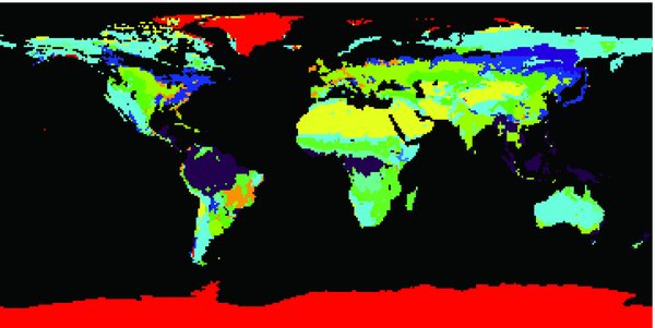
Figure 1. Terrain map of the Earth in the summer at 1° by 1° lat/long resolution. Each color represents a specific type of terrain (i.e., black = ocean, red = snow/ice, purple = evergreen broadleaf forests, yellow = desert, etc.). See Strahler et al. (1999) for further details.
Download figure:
Standard image High-resolution imageThe spatial size of each pixel on our map is adjustable and is generally set to 3° latitude by 3° longitude. This gives a good compromise between details (resolution) and the computational speed of the simulation. Each type of terrain is then assigned a standard reflectance spectrum for that type of terrain based on empirical data from the USGS Spectral Library2 5 (Clark et al. 2003). However in this paper the spectral information is not studied, and results are averaged over the bandpass.
The brightness of each location is the most difficult aspect to model as it depends upon both the angle of incidence of the solar light and the angle of reflection (both altitude and azimuth) toward the observer (Figure 2), and is different for each pixel. The functions that describe this are the bidirectional reflectance, the ratio of reflected to incident flux, and the bidirectional reflectance distribution functions (BRDFs), which describe the anisotropy of the reflected radiance. Two well respected discussions of this are to be found in Nicodemus et al. (1977) and Hapke (1993).
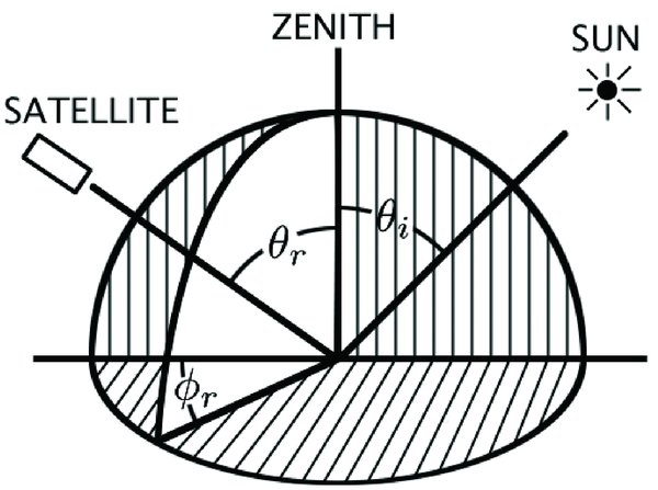
Figure 2. Diagram of the reflectance geometry.
Download figure:
Standard image High-resolution imageWe elect to use the BRDF developed by Manalo-Smith et al. (1998) as they were compared to models developed from data by the Earth Radiation Budget Experiment (ERBE) aboard Nimbus 7 (Jacobowitz et al. 1984) and designed to closely match the data. We choose to use these functions as they represent observed reflectance data from genuine Earth surfaces, rather than scattering theory based on idealized substances. These models also have the advantage of taking into account the change in reflectance due to different amounts of cloud cover as well as Rayleigh scattering in the atmosphere.
The functions include several parameters that vary depending on the type of the surface and include: ocean, land, snow and desert, as well as parameters for the amount of cloud coverage. The number of land types is less than that categorized by the MODIS data, and therefore we group several categories into a more general "land" classification. Since the BRDFs match well with the ERBE models, this lack of surface type variety does not affect our calculations of the Earth's disk-average reflectance. This loss of detail in land types could lead to some loss of detail in Earth's disk-averaged spectra. However, many of the land types would have similar reflectance spectra (e.g., Evergreen Needleleaf Forests versus Evergreen Broadleaf Forests), and thus this loss of detail in categorization would be small.
The details of these BRDFs can be found in Manalo-Smith et al. (1998). The equations have terms for cloud reflection, diffuse scattering, Rayleigh scattering and specular reflection. Specular reflection is the mirror-like reflection that occurs off of smooth surfaces such as water. This reflection has a high intensity and is highly anisotropic. The functions depend on the scattering angle (γ), the angle away from specular reflection (α), angle of incidence (θi), and the angle of reflectance (θr). They also contain six terms to represent constants assigned to best fit the functions to observed data and vary with terrain type. The last constant represents cloud cover amount over a particular location. Unfortunately, due to limited data, the reflectance functions were fitted to a finite range of angles, typically limited to solar zenith angles ≲75°. To calculate the reflectance of terrain at larger angles we simply assumed Lambertian reflectance with an appropriate albedo for each terrain type. The contribution from these points is typically minor. For specular reflection at high zenith angles we take the reflectance value at the maximum functionally valid solar zenith angle and scale it by the Fresnel reflectivity at the true angle. The set of functions also lacks a BRDF for a cloudy-snow terrain. As the effects of seasonal snow/ice are of interest we created a cloudy-snow reflectance by combining the functions for cloudy-land and clear-snow, weighted by the percentage of cloud cover.
2.1.2. Cloud Reflectance
Cloud coverage also plays a key role in reflectivity by decreasing the influence of the surface terrain type and increasing the overall brightness due to high albedo. Cloud coverage was applied using the D1 data set observations from the International Satellite Cloud Climatology Project3 (Schiffer & Rossow 1983). Global cloud coverage is compiled every 3 hr and has a spatial resolution of 280 km. The relatively high temporal resolution of these cloud maps allows our simulations to continuously update cloud coverage every 3 hr, giving us an accurate view of Earth even as weather systems evolve over short (for weather patterns) time scales. We use data from the entire 2004 year to accurately portray the evolution of clouds over a full orbit.
2.1.3. Simulating Diurnal Light Curves
Of primary interest to us is the unresolved light curve of an exoplanet as it rotates with new landforms and clouds come into the field of view. At a distance of ∼10 pc, the planet is unresolved, but the changing reflectance of the planet gives us clues to its geographic and atmospheric features. In order to calculate the disk-averaged reflectance of an exoplanet, the parameters of interest are the orbital longitude (i.e., phase) of the planet, the orbital characteristics, the location of the observer, the surface and cloud maps, and the reflectance functions. The orbital characteristics are left untouched from Earth's values, while, unless specified otherwise, the phase varies depending upon the day of year. The orbital inclination is always North-centric (0° corresponding to a face-on view of the North Pole and a 90° view corresponding to edge on), and the right ascension of the observer is 270° (opposite to the Sun on the summer solstice).
Each pixel on our model Earth calculates the local altitude and azimuth of both the parent star and the observer for each time step (ignoring the small effect of the parent star having a ∼30' angular width). If both objects are visible from that location (i.e., both have positive altitudes), then the angles (θi, θr, ϕr, γ, α) and the terrain type (including updated cloud/snow/ice coverage for that individual timestep) are fed into the reflectance functions and the reflectance is calculated for each observed pixel. This process is continued at every time step (usually between 15 minutes and 1 hr) for the specified observation length (typically either a day or a year). The reflectance at a given time step is calculated by taking the average of three reflectance values at times t and t ± Δt/2 (where Δt is the length of a time step). Thus, the code is run at a temporal resolution of double the desired observational resolution.
In this manner we take a spatially resolved model and simulate its unresolved reflectance at any orientation, orbital position, orbital phase, and observer location desirable at any time of year. An example of the diurnal light curve is shown in Figure 3 for an atmosphere-less Earth. The specifications for this observation were chosen to match Figure 1 from Ford et al. (2001). The light curve, though calculated by different techniques match very closely.

Figure 3. Diurnal light curve of the Earth at quadrature excluding both clouds and atmospheric reflectivity. Reflectivity is normalized to a full phase perfectly reflecting Lambertian sphere.
Download figure:
Standard image High-resolution image2.2. New Worlds Simulations
In order to describe the capability of an external occulter system to analyze the observed diurnal light curve we must first decide on the technical architecture of the observing system. We simulate an image with a 4 m telescope in the 0.3–1.0 μm bandpass behind a 50 m starshade at a distance of 70,000 km. The result is shown in Figure 4. These parameters were chosen to present a reasonable test case and do not indicate the final NWO system.
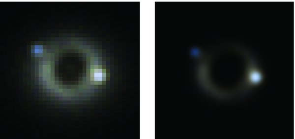
Figure 4. Simulated 4 m New Worlds Observer image of the habitable zone of an exosystem inclined at 30°. The central circular shadow is cast by the starshade, while Venus (3 o'clock) and Earth (10 o'clock) are clearly visible. Mercury is inside the inner working angle of the starshade and Mars is too dim to see by eye above the exo-zodiacal light. This image is cropped to show detail in the habitable zone and thus eliminates the otherwise bright outer planets. Colors are taken from Bowmaker et al. (1980) and are blue: 0.42 μm, green: 0.534 μm, red:0.563 μm. Intensities were squared to enhance contrast. Left represents the pixelated image while the right is smoothed.
Download figure:
Standard image High-resolution imageThe primary sources of noise in a New Worlds observation are direct solar light, reflected solar light from exo-zodiacal dust, and local zodiacal light. Each of these are discussed separately below.
2.2.1. Solar Light
New Worlds can accomplish direct observations of Earth-like planets via the use of a new type of external occulter known as a starshade. This starshade is shaped to cancel out diffracted light, leaving a shadow of ∼1010 suppression of the incident starlight. This amount of suppression will allow relatively easy observations of the planetary system. The amount of starlight suppression as a function of viewing angle was calculated by Cash (2006).
Introductory lab tests of starshades have been conducted recently in air by Leviton et al. (2007) and weak vacuum (∼1 torr) by Schindhelm et al. (2007). These tests have used a heliostat setup to illuminate a starshade with broadband solar light and measure suppression and contrast ratios. With starshades manufactured using a variety of techniques they have already produced suppression in the 106–108 range for the initial tests. Ongoing lab tests with better manufacturing of starshades are expected to produce even better results.
2.2.2. Zodiacal Light
The greatest obstacle to identifying planets in the habitable zone is the presence of zodiacal dust in the exo-system. The presence of exo-zodiacal light is modeled in our simulation using the software Zodipic developed by Moran et al. (2004). The exo-zodiacal light is the largest source of noise in our observations, and is thus one of the primary limiting factors in our ability to accurately interpret these diurnal light curves. The local zodiacal light is an additional source of noise with a brightness of approximately 23 mag arcsecond−2.
2.2.3. Other Sources of Noise
Our simulation also includes the secondary sources of noise from dark current and read noise set at current technological standards. For broadband photometry these sources are not significant.
3. ANALYSIS OF LIGHT CURVES
It is more illuminating to examine the evolution of a model Earth's light curve over the span of a year. To accomplish this, we ran the simulation over the entire 2004 year (leap day included), updating the stellar, planet, and observer positions and recalculating the observable surface features at every time step (typically an hour). The global cloud coverage was updated every 3 hr and global snow and ice coverage every day. We could then examine the evolution of a light curve as viewed by an observer, including any potential periodic effects due to cloud movement and seasonal changes.
The short-term variation in intensity of these curves (Figures 5 and 6) is due mostly to the diurnal cycle of reflectance (referred to in this paper as inherent variability), but also to noise from sources such as exo-zodiacal light and Poisson variation. When considering the full bandpass, the signal to noise varies from ∼1 to 10 over a full orbit at i = 90° when the planet is outside the inner working angle (IWA). These values (both S/N and IWA) depend both on the planetary system and on the technical details of the observing system (width of the bandpass, detector Q.E., etc.), and will change as the NWO optical system evolves. The inset plot in Figure 5 (top) shows a magnified view of 4 days of observation. Also plotted beneath these curves is the maximum variability in each day for both the inherent diurnal cycle and the realistic noised data.
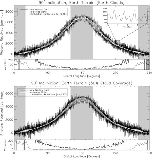
Figure 5. Reflectance over a full orbit as a function of cloud level for an Earth twin at 10 pc. Count rates are calculated from reflectance calculations convolved with high efficiencies of optics in the visible spectrum and a wide bandpass with dichroics and/or multiple detectors rather than single filter photometry. The white curve represents the inherent diurnal curve, while the black curve includes effects such as exo-zodiacal light and Poisson noise. The overall shape is due to the planet's changing phase as its orbits. The inset plot represents a magnification of 4 days of noiseless data to better show the hourly variations and daily pattern. The most interesting feature is the sharp increase variability at crescent phases (e.g., longitude ∼330°) shown in the bottom plots. These plots show the variability (as a percentage of intensity) due to both the inherent diurnal variation (gray) and convolved with realistic noise (black). The specular reflection off the ocean during crescent phases is the dominant source of surface reflection and is still noticeable even with Earth-like clouds (see Section 3.3). The gray areas indicate locations when the planet is unobservable behind the starshade (≲50 mas).
Download figure:
Standard image High-resolution image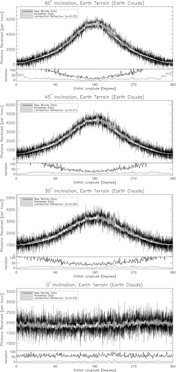
Figure 6. Light curve plots for various inclination systems. By i = 0° seasonal effects become noticeable as the observer is viewing the highly northern latitudes at small zenith angles (see Section 3.4).
Download figure:
Standard image High-resolution imageWe also observe how the light curve would be affected by various average cloud amounts (Earth-like and 50% average coverage). The reduced cloud coverage maps are created by taking the empirical ISCCP data and linearly scaling down to the desired cloud amount. Further studies may find that other techniques are better for modeling low cloud systems, but this basic approach is adequate for this study. The results are displayed in Figures 5 and 6 for inclinations of 90°, 60°, 45°, 30° and 0°. These curves do not include the complications due to the starshade blocking the planet's light at near full and new phases (these longitudes are marked in gray in Figure 5). To observe at these orbital longitudes, a system closer than 10 pc would be required, or the use of a different starshade geometry.
3.1. Variability
The light curve's hourly variability is a complicated indicator of the surface terrain. The variability is primarily due to differing cloud coverage and the variety of surface albedos where the cloud coverage is minimal. The presence of specularly reflecting surfaces can increase variability at crescent phases as can the cloud coverage for any particular day. The sources of noise (particularly exo-zodiacal light) also increase as Earth's angular separation from the star decreases at crescent phases.
Considering all of these contributions, the average daily inherent variability ( where
where  is the median reflectance value for the day) at i = 0° varies from ∼5% at full phase to 40% at crescent phases. While the realistic observational data vary from 5% to 100%. The daily maximum variability
  varies from 10% to 100% and 20% to >100% for inherent and observational data, respectively. The average daily variability gives an indication of the variety of cloud coverage and surface terrain, while the maximum daily variability is more sensitive to occasional spikes in the data such as those caused by specular features.
At an inclination of 0°, the average variability is 15% with no noticeable change between seasons. This average increases for systems with reduced cloud cover. Simulations run for conditions similar to Goode et al. (2001) give variations ∼16% compared to an observed value of 15%. For an Earth seen at quadrature, a typical day will show brightnesses ranging from 24.8 to 25.0 mag dimmer than the host star.
3.2. Rotation Rate
The New Worlds Observer mission gives us the opportunity to determine planetary rotation rates. Given hour-long exposures taken continuously for 5 days of a system at i = 0° we can analyze with good accuracy the periodic tendencies of the light curve. We first use an S/N of 20 to match previous studies. Given 100,000 runs starting at random orbital longitudes, we find that a simple Fourier power analysis indicates a 24 hr rotation rate for 75% of the runs, with 14% of the runs indicating a 12 hr rotation rate. This is not surprising given Earth consists of two main landforms and two main oceans. The failures are particularly noticeable at certain orbital longitudes, indicating that the cloud coverage for these weeks convolved with the particular viewing geometry lead to especially difficult cases to diagnose. At i = 90° we were successful 54% of the time for observations conducted while the planet was not obscured behind the starshade.
Similar simulations on a Pangea-type Earth (land to water ratio of 1/4) does not greatly improve our ability to correctly determine rotation rates at i = 0°, giving the correct rotation rate 80% of the time for random initial orbital longitudes.
The rotation rate of a water planet could be determined correctly via this method 93% of our runs, while for a completely land covered planet our success rate was 98%. For these two cases the change in reflectance is due solely to cloud coverage, thus our success is evidence of the general stability of large-scale cloud structures over the span of a few days. Given the hypothetical occurrence of a cloudless planet, the ability to correctly determine the rotation rates was 100%.
These results are consistent with the recent study done by Pallé et al. (2008). They were successful at a similar rate of 85% for exposures of 1.7 hr at an S/N of 20. At i = 90° their most successful parameters succeeded 38% (0% with all other parameters) of the time compared to our 54%. Thus, our results match reasonably well given similar S/Ns. Differences likely stem from the total observation time, exposure time, year of cloud coverage data, and general differences between models. A comparison of results is shown in Table 1 for the set of parameters that most closely resembles ours.
Table 1. Success Rates Compared to Previous Studies
| i | FFT This Paper | FFT Pallé et al. (2008) | Autocorrelation This Paper | Autocorrelation Pallé et al. (2008) |
|---|---|---|---|---|
| 0° | 75 | 85 | 76 | 80 |
| 30° | 62 | ⋅⋅⋅ | 85 | ⋅⋅⋅ |
| 45° | 60 | 66 | 84 | 85 |
| 60° | 56 | ⋅⋅⋅ | 81 | ⋅⋅⋅ |
| 90° | 54 | 38 | 83 | 85 |
Notes. Parameters for this table are 1 hr exposure, 5 days of data, and an S/N of 20. Parameters for Pallé et al. (2008) are 1.7 hr exposures, 2 weeks of data, and an S/N of 20. The numbers indicate success percentage, defined as 24 ± Δ hr where Δ is the exposure time.
Download table as: ASCIITypeset image
We experimented with different length exposures and found that 30 minute exposures reduced our overall ability to successfully determine the rotation rate to 62% of the runs at i = 0° due to the reduced S/N it would cause. Taking 3 hr exposures did not noticeably increase the success rate either.
We also attempt to determine rotation rates by way of an autocorrelation analysis. We find, as did Pallé et al. (2008), that the autocorrelation rarely (∼2%) makes the mistake of determining a 12 hr rotation rate. We also found an increase in success at determining a 24 hr rotation rate at high inclinations. Our numbers compare well for most similar set of parameters (Table 1). The failures in this type of analysis are spread evenly over orbital longitude. Overall, this technique appears to be more promising at all inclinations.
Our success rates indicate that with good reliability a New Worlds Observer mission could determine rotation rates in under a week of observing time. We found that to maintain success rates above 50% required an S/N in the 5–10 range with hour long exposures. Current estimations for NWO put it in this range for typical observations done with a wide bandpass. We show success rates for both techniques in this S/N range in Table 2. Interestingly, the FFT method outperforms the autocorrelation method in the low signal-to-noise regime. We also explore the more realistic case of allowing the signal-to-noise level to vary. We vary it on an hourly basis as in Figures 5 and 6. Thus, the more successful observations will occur at times of higher S/N which occur at fuller phases. Given a set of observations that detail the orbital parameters of a planet, the target can be revisited at an optimal time to obtain a success probability higher than listed below.
Table 2. Success Rates for Various S/Ns
| i | FFT (S/N = 5) | Auto (S/N = 5) | FFT (S/N = 10) | Auto (S/N = 10) | FFT (S/N = Variable) | Auto (S/N = Variable) |
|---|---|---|---|---|---|---|
| 0° | 32 | 15 | 63 | 42 | 53 | 39 |
| 30° | 33 | 21 | 56 | 61 | 50 | 42 |
| 45° | 35 | 28 | 51 | 65 | 45 | 41 |
| 60° | 38 | 30 | 51 | 64 | 38 | 48 |
| 90° | 42 | 35 | 49 | 66 | 45 | 39 |
Notes. Parameters for this table are 1 hr exposure, 5 days of data, and an S/N of 5, 10, or varying on an hourly basis. Numbers indicate success percentage, defined as 24 ± Δ hr where Δ is the exposure time. The 5 day periods are chosen to avoid the times when the starshade would obscure the planet in the i = 90° case.
Download table as: ASCIITypeset image
3.3. Detection of Liquid Surface Water
A key indicator of the presence of liquid surface water is the brightness variability at crescent phases. An Earth-like planet shows an increase in inherent daily variations by a factor of ∼6 at crescent phases than a completely land covered planet when observed at an inclination of 90°. The Earth-like planet is also approximately twice as bright when observed at this geometry (Figure 7). This is due to the intensity of specular reflection off the smooth ocean surface at high solar zenith angles. As the planet rotates this spot is periodically covered by land terrain or clouds, drastically diminishing the disk-averaged reflectance for a short time and causing high variability. At high system inclinations this observation is possible with Earth-like clouds. However, given the low signal strength of a planet at a crescent phase, noise will begin to dominate the observations and hide this inherent variability for an Earth twin at 10 pc. An example system with sufficient signal strength to allow an NWO detection of surface water would be one located at 7 pc with  of our zodiacal dust and a planet with ∼2 M⊕. Current solar system creating simulations typically create terrestrial planets (ranging from dry to ocean covered) with a range of masses between 0.23 M⊕ and 3.85 M⊕ (Raymond et al. 2004, 2006). Depending on the composition, this can cause an increased planetary radius by as much as ∼70% (Fortney et al. 2007), though we assume only a 1.33 R⊕ for this study. Thus our example system is well within the realm of reasonable models. It is difficult to predict the variety of exo-zodiacal distributions we will observe, but it seems likely that at least some systems, particularly older ones, will have lower levels. Another variable that would increase our detection ability would be an imaging system with greater than 70% overall throughput. As the New Worlds Observer will have high efficiency optics in the visible spectrum, this throughput is likely limited by the detector efficiency and could be quite high for a significant portion of the bandpass.
Figure 7. Comparison of an Earth-like planet with water oceans vs. an all land planet. The top plot shows a smoothed light curve of the two scenarios. The Earth-like planet is normally dimmer due to the lower albedo of water, but at crescent phases (orbital longitudes ⩾320) the intense specular reflection off of water makes the planet appear brighter than an all land planet. The Earth-like planet is almost twice as bright at crescent phases. The bottom plot shows the typical inherent daily variations, and shows a drastic increase in variations as the specular spot is temporarily obscured by clouds or continents. As mentioned in the text, noise will make this distinction challenging, but a NWO system should be able to accomplish this task given an observation at the correct orbital longitude for a plausibly favorable system.
Download figure:
Standard image High-resolution imageWe estimate that a New Worlds system can achieve this detection of water on the system described above, especially with 1.5–2 hr integrations. Longer integrations smooth out the very specular variations that we are interested in. Thus the strategy to discern liquid surface water is to watch the planet as it becomes a thin crescent and look for the brightness to trend brighter than the waterless curve would predict, and to have more significant variations than what would be caused simply by decreasing the signal to noise. Unfortunately, as the planet continues to a thinner crescent the signal to noise will drop too far, giving us only 1–2 weeks to obtain this observation. Additionally, this specular feature could be caused by a specularly reflecting terrain other than water (e.g., ice or another liquid).
Detecting liquid surface water requires an observing system that can observe at an angle of ∼60 mas from the host star. Thus, we stress the importance of having an observing system with a small inner working angle. The New Worlds Observer will be able to observe down to this IWA either due to the size/location of the starshade or through a dithering observing strategy that gives NWO an effective IWA much smaller than the static one (typically quoted ∼50–70 mas).
The increase in intensity at crescent phases due to specular reflection was also modeled by Williams & Gaidos (2008). However, they find it somewhat easier to make this detection by using models with a spatially constant cloud cover. Our models use actual cloud data (as detailed in Section 2.1.2), making this detection more difficult. Furthermore, our models are capable of showing the increase in hourly variation caused by ocean glint.
3.4. Detection of Seasons
The high increase in snow and ice terrain during the northern winter as well as the increase in visible land terrain due to Earth's obliquity has a strong effect on the orbital light curve of an Earth-like planet. The weekly average flux increases by ∼14% (Figure 6, bottom), with the two causes contributing roughly equally. This effect is plainly visible at low inclinations with typical clouds, and is still noticeable at up to 45° inclination given reduced cloud cover. Thus, we can deduce the presence of seasons on the planetary surface even without any resolving power. This is not surprising, as even a cursory look at snow/ice data indicates a high percentage of terrain change between seasons.
One could attempt to explain this increase in flux as being due to an eccentric orbit. As a planet approaches periastron, the overall reflectance will increase similarly to a planet experiencing winter. To investigate this possible source of confusion we have simulated an Earth with no obliquity and no change in seasonal ice, but with an orbital eccentricity. This comparison is illustrated in Figure 8. We show the cloudless models (left) for easy explanation, while the Earth-like models (right) show the realistic case.

Figure 8. Comparison of seasonal vs. eccentricity effects. Left pair represents cloudless planets while the right pair represents a planet with Earth-like clouds. The top rows are light curves for Earth-like orbital dynamics, while the bottom rows are light curves for planets with neither seasons nor obliquity, but with an orbital eccentricity.
Download figure:
Standard image High-resolution imageAlthough the two scenarios both show an overall increase of ∼14% (∼46% for cloudless) between summer/winter or apastron/periastron, the two scenarios are separable as there is a difference in the overall shape of the light curve. The Earth-like case has a relatively constant intensity (averaged over several days) until winter snow/ice, combined with an increase in visible land terrain due to Earth's obliquity, causes a strong increase. The seasonless/eccentric case shows this same increase at perihelion, but also shows a corresponding decrease during aphelion. Thus, the light curve of an eccentric orbit shows a much more sinusoidal shape than the light curve of a seasonal Earth.
For the realistic case with clouds, this shape contrast is still present, but more difficult to discern. However, one can still separate the two cases based upon how strongly a particular day's light curve correlates with other days. In the seasonless case, the observable land terrain is constant throughout the year (except for the changing obscuration via clouds). Thus, any particular day correlates much stronger with other days than it would be if seasonal and obliquity effects modified the viewable terrain. More obviously, the determination of orbital parameters from a few adequately spaced observations should give us detailed knowledge of the planet's eccentricity. Due to the relatively large change in brightness, a high S/N is not needed for the detection of seasons.
3.5. Albedo
The reflectance simulations do not measure the total amount of outgoing light (i.e., the albedo), however the curves can be fitted to the reflectance curves of Lambertian spheres of a specified albedo. The albedo fit is typically 0.29–0.36 assuming a known planetary radius. These numbers are only approximations but are in good agreement with the measured value of 0.297 observed by Goode et al. (2001).
4. SURFACE MAPPING
A goal of light curve analysis is the potential of inverting them to map the terrain of the reflecting planet. The majority of the light curve information is in the direction perpendicular to the lines of illumination. Due to Earth's obliquity and the system's inclination these are not exactly lines of longitude, however we will approximate them as such in this paper. There exists the strong probability that we can map out basic landforms in this dimension. Information along the crescents (which we will approximate as the latitude dimension) is sparse, limited only to what we can infer from seasonal changes in the light curve. Below, we compare three methods of mapping terrain: the specular method, the albedo method, and the hybrid method. These methods are applied to the favorable planetary system described in Section 3.3.
4.1. Inverting Light Curves—Cloudless Case
We begin our analysis with the easiest initial conditions. We examine a completely cloudless exo-Earth through a New Worlds Observer system at both 90° and 60° inclinations. This cloudless scenario, though not very realistic allows us to experiment with different techniques and determine how to best approach this task. Below we present some of our successful results.
4.1.1. Specular Method
As discussed earlier, observations at crescent phases can determine the locations of water by looking for spikes in reflectance from the bright specular reflection. By co-adding more than 7 days of data we attempted to reduce the noise contribution (as detailed in Section 2.2) to a minimum. We chose inclinations of 60° and 90° so that we are able to observe the majority of the Earth's surface over a full rotation.
The inversion algorithm for this method at present is a simple one that assumes that the peaks in brightness are due to specular reflection off water, while the dimmer reflectance occurs during times when land covers the location of specular reflection. Thus, the percentage of water in a longitudinal bin is simply the reflectance value scaled to the two extremes and is arbitrarily centered on the equator.
There will be an additional constant necessary to determine the correct land to water ratio. The shape of the continents remains the same regardless of this, but their latitudinal extent depends upon its accurate measurement. A lower limit on this constant could likely be accomplished simply by analyzing the variability increase of planets with different amounts of water, however a true estimation will likely be done via isostasy arguments, polarization measurements, and spectral analysis. That study is beyond the scope of this paper,
For an observer at a right ascension of 270°, the Earth appears in a new phase at the Summer Solstice. Approximately, 45 days before and after this is when an observer would see the specular reflection. We attempt the inversion at an orbital longitude of 40°, where the exo-Earth is outside the starshade's inner working angle (i.e., outside the gray areas in Figure 5) and the high variability due to specular reflection is still noticeable.
The map is then smoothed over 1° resolution to give more realistic shapes. The resulting inversions for both 90° and 60° inclinations are shown in Figure 9.
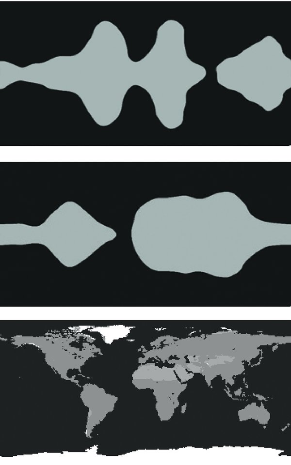
Figure 9. Top: specular inversion method of a system inclined at 90°. The location of specular reflection occurs on a belt centered at the Equator. Therefore, the map fairly accurately portrays the continents along this belt (South America and Africa), but is insensitive to the presence of other more northern continents. Middle: specular inversion method of a system inclined at 60°. This more accurately maps the northern continents, but ignores the southern/central land masses. This inversion appears more accurate as the majority of mass on our planet is in the Northern Hemisphere. Both these inversions do a reasonably accurate job of mapping the relative size of the land masses in their correct longitudinal location. Of course, without much information in the latitudinal direction, the shapes of these continents are not well matched. Bottom: map of Earth for comparison.
Download figure:
Standard image High-resolution imageOverall, the inverted map is a good indicator of the location of land masses and their relative sizes. It is a poor indicator of shape (as to be expected), and is also insensitive to land terrain outside the relatively small location of specular reflection. The land masses outside of this specular location will not be well represented. In fact, land terrain outside these regions would actually increase the reflectivity (due to their higher albedo than water for non-specular reflection), instead of decrease as this algorithm assumes. Thus, this method is a very good mapping tool along the belt of specular reflection (roughly 25° latitude in diameter), but is poor outside of this belt.
4.1.2. Albedo Method
A different inversion technique should be used when specular reflection does not dominate the overall brightness of the planet (orbital longitudes ∼40°–320°). The function simply assumes that the brightest observations correspond to those with the most land terrain, while the dimmer observation corresponds to the dark ocean (non-specular) reflection. Using these assumptions, we calculate the average land mass visible at each step in the orientation and again smooth it to 1° longitude resolution. The results are displayed in Figure 10 for systems inclined at both 90° and 60°. This method is less successful than the specular method.
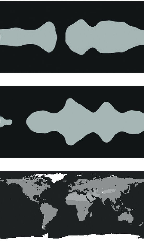
Figure 10. Top: albedo inversion method of an edge-on system. This technique does a moderately good job of mapping the relative sizes of continental land masses. Middle: inversion of a system inclined at 60°. This inversion is a poor fit to the real Earth. This failure is likely due to the presence of the Arctic ice that is visible from this inclination (but not from the previous one). Bottom: reference map of the Earth.
Download figure:
Standard image High-resolution image4.1.3. Hybrid Method
The hybrid method combines techniques from the previous two sections for observations at crescent phases. For bright reflectance values it calculates the percentage of the specular spot covered by land for values less than the maximum. For dim reflectance values it assumes that the specular spot (approximately 25° in diameter) is completely covered by land and any increase over this minimum is caused by more land mass outside the specular reflection spot. Thus in this instance additional land increases reflectivity. Theoretically, this method should accurately reproduce the "specular belt" as well as be somewhat sensitive to land masses outside this region. The results of the inversion for inclinations 90° and 60° are shown in Figure 11. This method produces the best results.
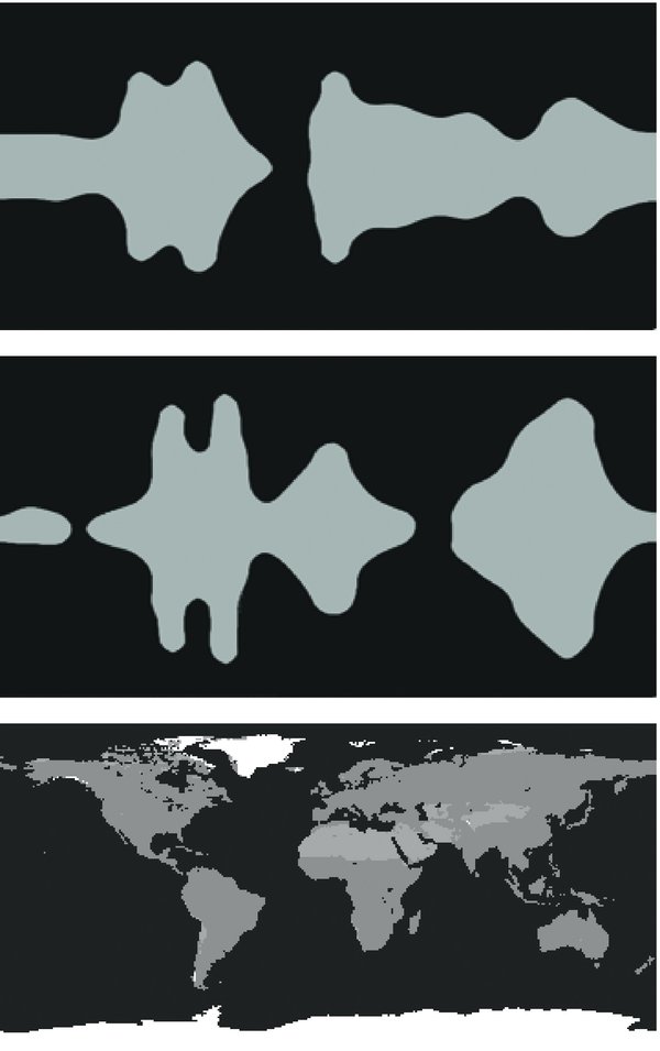
Figure 11. Top: hybrid inversion method for an edge-on system. This technique performs fairly well in identifying location and relative size of land masses. It is also sensitive enough to pick out minor variations—for instance, the separation between the Americas and the Indian Ocean. Middle: inversion for a system inclined at 60°. This map again shows the increased sensitivity, though it poorly maps the Atlantic Ocean. As with the previous method, this algorithm is somewhat deceived by the highly reflective Arctic ice. It should be noted that the longitudinal alignment process is difficult and is only accurate to ∼10° longitude. Bottom: reference map of the Earth.
Download figure:
Standard image High-resolution image4.2. Inverting Light Curves—Cloudy Case
To test a realistic case, we attempted the same inversions of an Earth with clouds. The real difficulty in this scenario is determining how much of the light curve is produced by ground reflection versus cloud reflection. This is especially challenging due to the high albedo of clouds. If cloud coverage were truly random, one could compare the reflectance at a particular rotation state over several days/weeks and select the minimum reflectance value. This would in theory give the most accurate reflectance of the Earth's surface and lead to the best inversion results. However, the average cloud cover over a particular location on Earth is not random with respect to latitude and longitude. As illustrated in Figure 12, the average cloud cover varies drastically over Earth.

Figure 12. Average cloud cover over the entire 2004 year. White indicates highest concentration of clouds. Note the relative scarcity of clouds over Africa as compared to Asia.
Download figure:
Standard image High-resolution imageThe nonrandom nature of cloud cover with respect to longitude makes it difficult to reduce cloud reflectance. The best we can hope to accomplish is to minimize the cloud component by taking the minimum reflectance of each rotational state over the period of several days. This introduces a systematic error that is unavoidable without prior knowledge of the cloud pattern. One potential solution is to use the planet's observed color variation (Hamdani et al. 2006) as a diagnostic for cloud coverage.
If a large percentage of the planet is illuminated and visible (i.e., toward a full phase), then these changes will be minimal as the reflectance will be constructed with a large fraction of the Earth's surface, thereby making fractional changes in average cloud cover small. Therefore, we will be most effective in reducing cloud cover by considering thin crescents. This leads us to use the specular method instead of the albedo method.
Unfortunately, this method has little success at any phase brighter than the thinnest crescent. At 90° inclination no observing geometry gives an even approximate match to Earth's surface. At 60° inclination we obtained some recognizable features at a very thin crescent. Starting at an orbital longitude of 5° and observing for 2 weeks gives us the basic distribution of mass over the surface (Figure 13). This requires observing at an angle <10 mas away from the host star, which will be particularly challenging for any observing system even before considering the low S/N expected at this location. This success is also contingent upon reducing the noise in the system. Though several possibilities exist to accomplish a reduced noise system (chiefly reduced exo-zodiacal dust), the current NWO system will not be able to successfully accomplish inversion of planets with Earth-like clouds. This is due to both the convolution of ground and atmospheric reflectance and the relatively high level of noise.
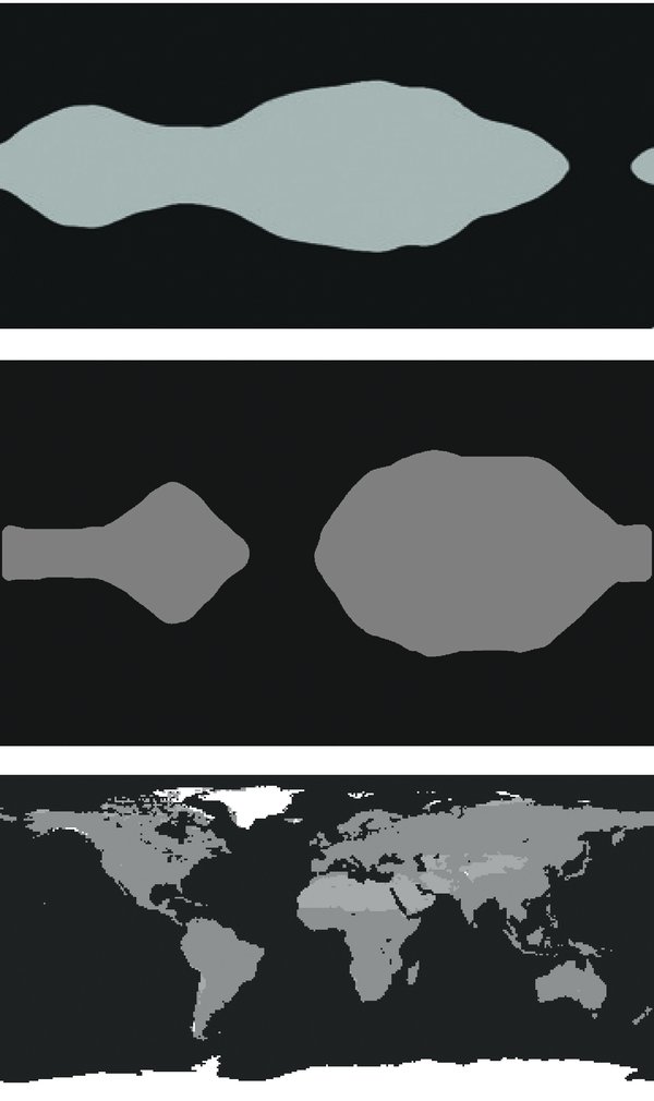
Figure 13. Top: specular inversion technique performed on a cloudy exo-Earth inclined at 60°. This example captures a general distribution of land over the Earth's surface, but is crude overall approximation, failing to identify even the Atlantic ocean. It also relies upon the unrealistic observation geometry. Middle: specular inversion technique performed on a reduced cloud level (25%) of an exo-Earth inclined at 60°. This example performs significantly better and is potentially obtainable with NWO. Bottom: map of the Earth for reference.
Download figure:
Standard image High-resolution image
The inversion failure at full cloud levels does not necessarily eliminate the practicality of this technique. It is quite possible that we may observe planets with reduced cloud levels. To investigate our inversion abilities with reduced clouds we simulated our favorable planetary system (2 M⊕ at 7 pc with 1/3 zodi) with an average planetary cloud cover of 25%. At i = 60° we were fairly successful, obtaining a passable distribution of land-mass over the two main continent systems as well as the correct location of the Atlantic Ocean (Figure 13, middle). This appears to be the most ground information that we can extract from the diurnal light curve without better knowledge of the atmospheric component. This inversion was accomplished at an orbital longitude of 40°, outside of NWO's effective IWA. Results at 50% cloud cover were less promising, indicating that this technique relies upon cloud levels less than half of Earth-like clouds.
5. SUMMARY
We have constructed a fully empirical code to model the Earth's diurnal reflectance. We use observational data from several Earth monitoring satellites and analytic BRDFs. This code is capable of generating reflectance values for the Earth at any orientation, time of year/day, and observer location. By running this code for an entire year, with continuously updating cloud/snow/ice coverage maps, we generated accurate orbital light curves for a variety of inclinations and cloud cover amounts through a simulated New Worlds Observer. We have determined that with Earth-like cloud cover an observer can likely identify water via its specular reflection at inclinations near 90° for our favorable (but plausible) test scenario (a 2 M⊕ at 7 pc and a  exo-zodiacal dust distribution). The specular reflection is noticeable due to both an increase over expected brightness at crescent phases and an increase in hourly variability. This detection does not appear to be possible for our less favorable systems.
With either a Fourier power spectrum or autocorrelation analysis, a New Worlds Observer can accurately determine the rotation rate of this exo-Earth with a success rate of ∼30%–80% with only 5 days of observations depending on the signal to noise of the observation. The FFT analysis often returns a 12 hr rotation rate, while the autocorrelation analysis typically performs at a slightly higher success rate. These success rates are for our less favorable Earth-twin in a Solar System twin at 10 pc scenario. Additionally in this scenario, an asymmetry in the light curve due to the obliquity/seasonal snow is detectable with Earth-like clouds at low inclinations.
An analysis of diurnal light curves indicates that it may be possible to invert these curves to determine a basic longitudinal map of planetary terrain. We use three techniques to attempt to map an exo-Earth. The hybrid technique, used on a simple cloudless Earth for testing purposes, seems to map the location and relative sizes of the continents reasonably well given the difficulties involved. It is capable of sufficient detail down to the level of separating the Americas (though it does not have the information to center them at the correct latitude). Analysis on a realistic system using real cloud data produces far worse fits. No realistic observing geometry with NWO seems to produce a successful inversion at full Earth-like cloud levels using current techniques. However, at reduced cloud levels (less than half of Earth-like clouds), our inversions were far more successful. Thus given our favorable solar system scenario (or equivalent), NWO will be able to create crude planetary surface maps for planets with less than half of Earth clouds. Though always open to interpretation, these inversions would give us plausible surface maps decades before we have the telescope capability to resolve surface features on these planets.
Other potential diagnostic tools include: spectroscopic observations to help break the degeneracy between amount of land visible and albedo of land features, the overall color of the planet to give us an indication of instantaneous cloud coverage and polarimetric observations to distinguish between high albedo features and specular reflection off an ocean surface. More accurate models require better BRDF (particularly at high solar zenith angles) and more detail on how various cloud levels modify the reflectance. Additionally, more modeling must be done of exo-zodiacal light to study the detection and characterization of planets at crescent phases.
In order to extract information from a diurnal analysis, the observing system needs to achieve a broadband S/N of approximately 5–10 in an hour at any available phase to have ⩾50% success at determining the rotation rate of a planet. Seasonal variations will be noticeable with much cruder observations (S/N ≳3). The detection of surface water and the mapping inversion techniques also require S/Ns in the 5–10 range or higher in 1–2 hr. This is more difficult to achieve as they require this S/N at a crescent phases when the planet will appear dimmer.
We thank the NASA Institute for Advanced Concepts and NASA grants NNG05WC11G and NNX08AL70G for support of this work.
The ISCCP D1 data were obtained from the International Satellite Cloud Climatology Project data archives at NOAA/NESDIS/NCDC Satellite Services Group, ncdc.satorder@noaa.gov, on 2005 January.
Footnotes
- 1
- 2
- 3