


ABSTRACT
We determine the mass of the black hole at the center of the spiral galaxy NGC 4258 by constructing axisymmetric dynamical models of the galaxy. These models are constrained by high spatial resolution imaging and long-slit spectroscopy of the nuclear region obtained with the Hubble Space Telescope, complemented by ground-based observations extending to larger radii. Our best mass estimate is M• = (3.3 ± 0.2) × 107 M☉ for a distance of 7.28 Mpc (statistical errors only). This is within 15% of (3.82 ± 0.01) × 107 M☉, the mass determined from the kinematics of water masers (rescaled to the same distance), assuming they are in Keplerian rotation in a warped disk. The construction of accurate dynamical models of NGC 4258 is somewhat compromised by an unresolved active nucleus and color gradients; the latter caused by variations in the stellar population and/or obscuring dust. Depending on how these effects are treated, as well as on assumptions about the ellipticity and inclination of the galaxy, we obtain black hole masses ranging from 2.4 × 10⁷ M☉ to 3.6 × 10⁷ M☉. This spread is mainly due to uncertainties in the stellar mass profile inside the central 2'' (∼70 pc). Obscuration of high-velocity stars by circumnuclear dust (possibly associated with the masing disk) could lead to an underestimate of the black hole mass, which is hard to correct. These problems are not present in the ∼30 other black hole mass determinations from stellar dynamics that have been published by us and other groups; thus, the relatively close agreement between the stellar-dynamical mass and the maser mass in NGC 4258 enhances our confidence in the black hole masses determined in other galaxies from stellar dynamics using similar methods and data of comparable quality.
Export citation and abstract BibTeX RIS
1. INTRODUCTION
The characterization of massive dark objects (hereafter "black holes") at the centers of nearby galaxies has advanced considerably in the past decade. Nonetheless, the dynamical modeling of both stellar and gas kinematics remains subject to uncertainties. These can arise from, among other things, systematic uncertainties and noise amplification in the deprojection of the observables from two to three dimensions, the presence of dust that can affect both the mass-to-light ratio (M/L) and the observed kinematics, variations in M/L due to stellar population gradients, and the presence of nonstellar point and/or continuum sources in the central galactic regions which may swamp the light from the surrounding stars or gas. Gas kinematics can also be affected by nongravitational forces, random velocities, and pressure support, which are difficult to model accurately, while the complex phase-space structure of stellar orbits can make it difficult to properly sample initial conditions and the phase-space density distribution of the orbits in (stellar) galactic equillibria. Reverberation mapping presents a third possibility for determining black hole masses but comes with its own set of limitations (e.g., Blandford & McKee 1982; Peterson 1993; Netzer & Peterson 1997; Gebhardt et al. 2000b).
It is, therefore, desirable to test the reliability of these methods. Unfortunately, comparing stellar-dynamical estimates to gas-dynamical estimates of black hole masses is not usually possible, as few galaxies have properties that permit more than one method to be applied with confidence. Even in those cases, where it is possible, a detailed comparison is not always illuminating due to uncertainties in the measurements. One case where gas-dynamical and stellar-dynamical mass measurements are available for the same galaxy is not reassuring: the gas-dynamical mass for the black hole in IC 1459 is a factor of ∼5 smaller than the stellar-dynamical mass (Verdoes Kleijn et al. 2000; Cappellari et al. 2002). Better agreement, within a factor of ∼2, was found between the mass estimate of the black hole in Centaurus A by Silge et al. (2005) from stellar dynamics, and by Marconi et al. (2006); Neumayer et al. (2007) from gas dynamics. Another case with broad agreement but large uncertainty is NGC 3379, where Shapiro et al. (2006) found a best fit mass of 1.4 × 10⁸ M☉ (with large errors), compared to (2.0 ± 0.1) × 108 M☉ from gas—both consistent with the stellar-dynamical results of Gebhardt et al. (2000b). Even in the case of the supermassive black hole in the nucleus of our own Milky Way Galaxy, the mass estimates from individual stellar orbits (Ghez et al. 2005) and from a statistical analysis of radial velocities and proper motions (Chakrabarty & Saha 2001) differ by about a factor of 2.
NGC 4258 presents an exceptional opportunity to test the reliability of black hole mass estimators. Miyoshi et al. (1995); Herrnstein et al. (1999) used the Very Long Baseline Array (VLBA) to observe water maser emission in a thin, warped, and nearly edge-on gas annulus located at 0.16–0.28 pc from the center of this galaxy, and determined that a central black hole with a mass M• = (3.9 ± 0.1) × 107 M☉ is needed to account for the observed velocity profile, proper motions, and accelerations. This black hole mass is thought to be quite reliable for several reasons. (1) The maser-emission lines are both strong and narrow, lending themselves to VLBA observations of much higher resolution than possible with the Hubble Space Telescope (HST) or ground-based telescopes. (2) The masers seem to lie in a disk that is very thin (height/radius ≈0.02), so the corrections to the rotation curve due to pressure or random velocities are negligible. (3) Most importantly, the maser velocities scale very nearly as v(r) ∝ r−1/2 with distance r from the center, so that they exhibit an almost perfect Keplerian motion, which makes the deduction of the black hole mass easy and almost free of assumptions. (4) Finally, the measurements of the mass and distance from the radial velocities, proper motions, and accelerations of the masers are all consistent. More recently, Herrnstein et al. (2005), using a maximum likelihood analysis of the maser positions and velocities, quantified the deviation from Keplerian motion. A number of different models that can explain this discrepancy yield central masses in the range (3.59–3.88) ×107 M☉ rescaled to a distance of 7.28 Mpc. The warped disk model, which the authors consider the most probable, implies M• = (3.82 ± 0.01) × 107 M☉ at this distance.
In this paper, we estimate the mass of the central black hole of NGC 4258 via modeling of the stellar dynamics of the galaxy. This is accomplished using the orbit superposition tools developed by our collaboration (the "Nuker" team; Gebhardt et al. 2000a; Bower et al. 2001; Gebhardt et al. 2003; Thomas et al. 2004). Alternative orbit superposition tools have been developed by van der Marel et al. (1998); Cretton et al. (1999); Valluri et al. (2004). Because the maser black hole mass estimate seemed very accurate, we intended this to be a thorough, end-to-end test of the accuracy of our method, at least for this galaxy. Unfortunately, we encountered a number of problems that hindered our ability to determine unambiguously the mass–density profile in the central region of the galaxy. In particular, (1) it was not possible to accurately subtract the light of the unresolved active galactic nucleus (AGN) at the center of the galaxy to recover the underlying stellar luminosity profile; (2) it was not possible to reliably determine the stellar M/L profile within ∼2'' of the nucleus due to a color gradient, presumably caused by diffuse dust and/or a spatial variation in the stellar population; and (3) it was not possible to estimate the extinction caused by a compact dust patch near the nucleus, which may be obscuring light from fast-moving stars very close to the black hole, thus causing a systematic underestimate of the black hole mass.
Despite these difficulties, our "most trusted" estimate, M• = (3.3 ± 0.2) × 107 M☉, is in reasonable agreement with the maser mass estimate. The quoted error margin corresponds to the "1σ" confidence band, and reflects statistical errors only. Uncertainties in the mass profile discussed in the previous paragraph widen the error margin to 2.4 × 10⁷ M☉ < M• < 3.6 × 10⁷ M☉. This range still does not include the potential effect of obscuring circumnuclear dust, which cannot be easily estimated, or any other systematic effects such as deviations from axisymmetry that cannot be properly treated by our dynamical modeling method. These factors are discussed in detail in the following sections.
Pastorini et al. (2007) estimate the mass of the black hole in NGC 4258 using gas kinematics, but their 95% confidence intervals span a factor of 10 in mass, so this is not a strong test of the reliability of black hole mass estimates.
For this work, we use 7.28 Mpc for the distance to NGC 4258 (Tonry et al. 2001), which is in excellent agreement with the maser-derived distance of 7.2 Mpc. At that distance, 1'' ≃ 35 pc.
In Section 2, we present the photometric and kinematic data sets, which consist of HST WFPC2 and NICMOS imaging and STIS spectroscopy, complemented by ground-based imaging and long-slit spectroscopy that extend data coverage to larger radii. We discuss the large-scale morphology of the galaxy in Section 3, mainly as it pertains to the determination of the contribution of the stars to the gravitational potential. In Section 4, we consider the consequences of the color gradient in the central 2''. Section 5 presents the dynamical models. We conclude in Section 6.
2. OBSERVATIONS AND REDUCTION
2.1. Photometry
Here, we describe the acquisition and reduction of the photometric data, which are needed mainly to determine the stellar mass distribution and the kinematic-tracer profile, in the way described in Sections 5.1 and 5.4.
A journal of the imaging observations, from which the surface photometry was derived, is shown in Table 1. A wide variety of data are available in different colors, both from HST and the ground. For reasons explained in Section 4.1, we produced three luminosity profiles. (1) The near-infrared (NIR) profile was created by combining ground-based and HST J-, H-, and K-band images, as described in Section 2.1.1. (2) The V-band profile was generated from images in the V-band (HST) and in the R-band (ground based), as described in Section 2.1.2. (3) The I-band profile was created from the HST I-band image, as described in Section 2.1.2. Although this image was saturated in the nucleus, it was useful to consult for the luminosity weighting (normalization) of the line-of-sight velocity distributions (LOSVDs), as it identifies the kinematic tracer population (Section 5.4).
Table 1. Journal of Imaging Observations of NGC 4258
| Instrument | Filter/Band | Radial Range | Source |
|---|---|---|---|
| HST NICMOSa | F110W, F160W, F222Mb | r < 9'' | Chary et al. (2000) |
| KPNOc 2.1-m | K | 2'' ⩽ r < 32'' | This paper |
| 2MASSd | J, H, K | r ⩾ 32'' | Jarrett et al. (2003) |
| HST WFPC2e | F791Wf | r < 9'' | Cecil et al. (2000) |
| MDM 1.3-m | R | r ⩾ 9'' | This paper |
| HST WFPC2 | F547Mg | r < 9'' | This paper |
Notes. aNear Infrared Camera and Multi-Object Spectrometer. bCorresponding, approximately, to the J, H, and K bandpasses, respectively. cKitt Peak National Observatory. dTwo Micron All Sky Survey. eWide Field and Planetary Camera 2. fCorresponding, approximately, to the I bandpass. gCorresponding, approximately, to the V bandpass.
Download table as: ASCIITypeset image
2.1.1. Reduction of the J, H, and K-Band Data
The Two Micron All-Sky Survey (2MASS) J-, H-, and K-band images (Figure 1, top row) were kindly provided to us by Tom Jarrett (Jarrett et al. 2003), and extend out to R ≈ 8 6 from the center14. For the morphological study of the large-scale properties of the galaxy (Section 3), the signal-to-noise ratio (S/N) was boosted by constructing a composite J + H + K image, which was then smoothed with a Gaussian point-spread function (PSF) having full width at half-maximum (FWHM) of 7'' for r ⩽ 60'' and FWHM = 11'' for r > 60''. The 2MASS K-band image was reduced in a manner similar to that of the J + H + K image. It proved to have a sufficiently high S/N to give a reasonably adequate measurement of the outer disk. A comparison of the K-band and J + H + K-band photometry provides an estimate of the uncertainties; these are dominated by the effects of patchy star formation and other irregularities, not by photon statistics. Therefore, we decided to discard the J + H + K-band profile as a tracer of stellar mass in the dynamical modeling, and to use the K-band profile instead, as being less affected by these irregularities.
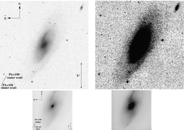
Figure 1. Ground-based NIR images of NGC 4258 identifying large-scale morphological characteristics of the galaxy: The bulge (PA ≃ 146°), which is embedded in the inner oval disk (PA ≃ 156°); the weak bar (PA ≃ 11°); and the outer oval disk (PA ≃ 150°). Top left: 2MASS composite J + H + K image. Intensity is proportional to the square root of surface brightness to illustrate the bulge and the small bar. The scale is 1'' pixel−1 and the image size is 171 × 171. Top right: As before, but intensity is proportional to surface brightness; the inner oval disk is now saturated and the outer oval disk becomes more prominent. Bottom left:K-band image using SQUID on the KPNO 2.1 m telescope. Intensity is proportional to the square root of surface brightness to illustrate the bulge. The scale is 0 69 pixel−1 and the image size is 59 × 59. Bottom right: As before, but intensity is proportional to surface brightness to illustrate the weak bar.
Download figure:
Standard image High-resolution imageThe Kitt Peak National Observatory (KPNO) 2.1-m telescope K-band image extends out to R ≈ 3' from the center (Figure 1, bottom row). Comparison of the 2MASS K-band profile with the KPNO K-band profile, which has a higher spatial resolution, showed that the 2MASS profile is affected by smoothing only at r < 32'', so the 2MASS profile was truncated inside this radius. Thus, the KPNO profile was used for 2'' < r < 32'' and the 2MASS profile at r ⩾ 32''.
Chary et al. (2000) obtained HST NICMOS images of NGC 4258 in bandpasses that approximate J, H, and K. Eric Becklin and Ranga Chary kindly made the reduced images available to us (Figure 2), along with the corresponding PSF images. Details of the reductions can be found in Chary et al. (2000). The HST WFPC2 V-band image (Section 2.1.2) shows extensive dust at r ≳ 2'' on the SW side of the center and a few thinner dust patches on the NE side. There is also a scatter of faint sources in the bulge, apparently associated with some ongoing star formation. In the NICMOS K-band image, these faint sources are not visible, and the dust patches on the NE side are essentially invisible as well. However, the dust on the SW side, although less conspicuous in K than in V, remains a substantial problem that we had to correct. After considering a number of alternatives, we chose the strategy of creating a symmetrized image of the galaxy, whereby the southwest (SW) side was replaced with the northeast (NE) side flipped (not rotated) across the major axis. As a check, the profiles from both the symmetrized and the unsymmetrized K-band images were compared and found to agree extremely well at r ≲ 2''. Therefore, this symmetrization is not a factor in the V − K color gradient discussed in Section 4.1. We applied the same procedure to the J- and H-band images, as well.
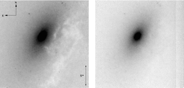
Figure 2. HST NICMOS images of NGC 4258 in the J band (F110W; left) and in the K band (F222M; right), from Chary et al. (2000). In both images, the scale and size are ∼0038 pixel−1 and ∼21'' × 21'', respectively. The images are not deconvolved. Intensity is proportional to the square root of surface brightness. A band of data is missing on the right side of the K-band image. For the extraction of stellar mass profiles from these images, the dust on the SW side was corrected by replacing the SW side of the galaxy with the NE side flipped across the major axis.
Download figure:
Standard image High-resolution imageThe nucleus of NGC 4258 emits broad permitted lines (Ho et al. 1997), and is classified as a Type 1.9 Seyfert. The AGN at the center is very red (Chary et al. 2000) and, in the K band, it appears as a bright, unresolved point source that clobbers the central brightness distribution of the stars and needs to be subtracted. Unfortunately, the PSF provided by Chary et al. (2000) was determined using the TinyTim routine and not from actual images taken at the same time as the galaxy observations. It proves to be a mediocre match to the AGN at r < 02, in the sense that there is a residual diffraction pattern no matter how the PSF is scaled. We applied the following procedure to improve the quality of the PSF subtraction (see Figure 3). Using VISTA (Lauer et al. 1983), we scaled the TinyTim PSF image by various factors and measured the resulting surface brightness profiles in the residual image using the unsymmetrized galaxy image. We also examined the residual images to see which ones had the small-scale structure, illustrated in the top-left image of Figure 3, optimally subtracted. Most of the weight in the choice of the final PSF scale factor came from how well the first diffraction ring of the AGN was subtracted. The scale factor that we finally adopted in this way yields ellipticity and position angle profiles that are both smooth and well behaved, which is reassuring. This is not the case with scale factors that differ by more than ±10% from the adopted value. However, ultimately no value of the scale factor allows both a convincing subtraction of the first diffraction ring and a smooth profile at r < 0 2 that follows the power law seen at a larger radii. This is probably a result of the imperfect match of the TinyTim-generated PSF to the K-band data. It is unlikely that a real galaxy feature is involved, considering that no such feature is detectable in the higher resolution V-band image in the radial range 0 05 < r < 0 2 (see Section 2.1.2).
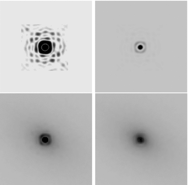
Figure 3. HST NICMOS K-band images of the central 5 7 × 5 7 of NGC 4258, adapted from the images provided by Chary et al. (2000). North is up, and East is to the left. Top left: The TinyTim model PSF shown at a nonlinear stretch (higher contrast at lower surface brightnesses) to emphasize the small-scale features. Top right: Same as before, but now scaled to the galaxy image and at the same linear stretch as in bottom row. Bottom left: The galaxy before PSF subtraction; the AGN is evident. Bottom right: The adopted PSF-subtracted galaxy image that was used to provide the central brightness profile in the K band. In the end, the AGN could not be subtracted well enough in K, and the J-band profile was used for r < 0 2.
Download figure:
Standard image High-resolution imageWe also applied 40 iterations of Lucy deconvolution (Lucy 1974; Richardson 1972) to the HST NICMOS J-, H-, and K-band images using the PSFs from Chary et al. (2000). Because the PSFs are not ideal, we applied the deconvolution to images with the PSF of the AGN subtracted as explained above. Still, the deconvolved K-band image showed bad "ringing," so we truncated it inside r = 0 46. The J-band profile appeared better behaved, at least partly since the AGN is much dimmer at this bluer wavelength, although there was also some sign of a residual AGN at r < 0 1. The J-, H-, and K-band deconvolved profiles agree very well at r ≳ 0 5, where the AGN is not a problem, and the ellipticity profiles are all well behaved.
Based on the preceding analysis, we decided (1) to use the original (not deconvolved) K-band photometry for r ⩾ 2 8 (KPNO data at 2 8 ⩽ r < 32'', and 2MASS data at 32'' ⩽ r ⩽ 560''), (2) to average the deconvolved NICMOS K- and J-band photometry for 0 2 ⩽ r < 2 8, and (3) to use deconvolved J-band data for 0 038 ⩽ r < 0 2 in order to avoid the AGN as much as possible. The resulting profile is shown in Figure 4. However, even in J, the points at r < 0 11 are probably still affected by the AGN. We elaborate on this point in Section 4.2.
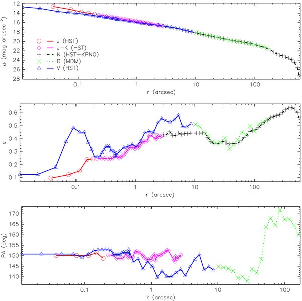
Figure 4. NGC 4258 major-axis surface photometry after subtraction of prominent dust lanes, and correction for the AGN. The radius (r) is measured along the major axis. All HST profiles are deconvolved for r < 3''. Top: NIR (J, J + K, K) and optical (V, R) surface brightness profiles. The R-band profile is calibrated using the HST V-band zero point between r ≃ 5'' and 7''. The NIR profiles are scaled to match the optical profile at large radii to illustrate the absence of major color gradients in the disk. The almost power-law profile at r ≲ 40'' belongs to the bulge. Only data out to r ≈ 150'' are used for the dynamical modeling. Middle: The ellipticity as a function of radius. Bottom: The position angle of the major axis as a function of radius.
Download figure:
Standard image High-resolution image2.1.2. Reduction of the V- and I-Band Data
We used the MDM 1.3 m telescope to obtain an image of the galaxy in the R band (Figure 5). The image was reduced and dust-clipped in the usual way. The luminosity profile was then extracted and matched to the V-band HST profile, discussed below, in the range 5'' ≲ r ≲ 7'', using a V-band zero point. There were no significant color, ellipticity, or position angle (PA) gradients between the V-band and R-band profiles over the radial range in which they were matched. Henceforth, we will refer to this composite profile, made by stitching together the HST V-band profile with the R-band profile shifted by a constant offset, as the V-band profile. It extends out to r ≈ 150''.
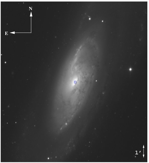
Figure 5. Ground-based image of NGC 4258 in the R band taken with the MDM 1.3 m McGraw Hill telescope. The square is centered on the nucleus, and is 8'' on a side. The scale of the CCD was 0508 pixel−1. A logarithmic stretch has been applied, and set to prevent "overexposure" of the bulge region.
Download figure:
Standard image High-resolution imageWe obtained HST WFPC2 images of the NGC 4258 nucleus through the F547M filter under program GO–8591. The F547M filter was selected to exclude any bright emission lines associated with the AGN; it is roughly equivalent to a narrow V-band filter, and is referred to as such in the remainder of this paper. The galaxy was centered in the PC1 chip and dithered in a 2 × 2 square raster of ∼0.5 pixel steps over four separate 400 s exposures to maximize the spatial resolution of the complete data set. The four dithered images were combined into a single Nyquist-sampled "super image" using the algorithm of Lauer (1999a), which provides for the optimal combination of undersampled images without any associated degradation of the resolution. This final image has a pixel scale of 0 0228, twice as fine as that of the original images. However, the Nyquist image remains modulated by the HST PSF; thus, it was deconvolved prior to further analysis using 80 iterations of the Lucy (1974); Richardson (1972) algorithm. The PSF was estimated using the TinyTim package, but incorporates the WFPC2 pixel-response function recovered by Lauer (1999b). The final deconvolved V-band image of NGC 4258 is shown in Figure 6.

Figure 6. HST WFPC2 image of NGC 4258. The large panel shows the central 256 × 256 pixels of the deconvolved F547M Nyquist-sampled image. It corresponds to 128 × 128 PC1 pixels, or 5 84 × 5 84. An arbitrary logarithmic stretch has been applied. The small upper-right panel is the central 1 48 × 1 48 (64 × 64 subpixels) of the same image, magnified by a factor of 2 compared to the larger panel. Again a logarithmic stretch has been applied, but with greater contrast over the nuclear region. The bottom-right panel shows the same region divided by a model reconstructed from the surface photometry. North is up and East to the left.
Download figure:
Standard image High-resolution imageThe V-band surface brightness profile of NGC 4258, shown in Figure 4, was estimated from the F547M Nyquist image using a combination of the high-spatial resolution algorithm of Lauer (1985) and the least-squares estimator of Lauer (1986). The patchy dust seen throughout the bulge of NGC 4258 complicates measurement of the brightness profile; as is visible in Figure 6, there is a compact dust feature just slightly offset from the nuclear source that was especially problematic. For all dust features other than the central patch, pixels affected by dust could simply be excluded from the least-squares profile estimator. In practice, this was done iteratively by comparing the image to a model reconstructed from the profile to isolate faint dust absorption that may have been missed during the initial inspection of the image. Unfortunately, pixels could not be masked out of the high-resolution profile algorithm, which is used in preference to the least-squares estimator for r < 0 5, so the nuclear dust patch was first filled in with an estimated correction provided by the lower resolution least-squares algorithm. This initial correction was then refined by replacing it with an improved estimate provided by a model reconstructed by the high-resolution profile.
Figure 6 shows the central portion of the V-band image divided by a model reconstructed from the final brightness profile. Apart from the nuclear dust patch, the residuals are flat, showing that the brightness profile extracted is faithful to the central structure of NGC 4258. The nuclear dust patch, itself, is clearly compact, affecting only a single quadrant of the nucleus, which again allowed it to be isolated from the profile estimation. As a "sanity check" on the brightness profile, we compared the profile to an intensity trace taken along the bulge semimajor axis on the side of the nucleus opposite the nuclear dust patch. The two measures agreed extremely well, showing that the final profile is not strongly affected by any residual dust features or the pixels excluded from the analysis.
In addition to the HST F547M data, we also analyzed two archival PC1 F791W (I-band) images obtained by Cecil et al. (2000) under program GO–6563. Unfortunately, both images were saturated at r < 0 09 from the nucleus, and thus provide information only at somewhat larger radii. The images were combined and deconvolved; however, without a full accounting of the light contributed by the nucleus, the I-band profile should be regarded with caution for r < 0 5.
Using the F547M and the F791W images, we created a F547M/F791W color map of the nuclear region of the galaxy, approximating V − I (Figure 7). The color map shows more clearly the distribution of dust in the center, and will be further discussed in Section 4.1. A larger scale view of the central region of the galaxy is shown in Figure 8, which is a composite color image created by combining the F547M and the F791W images along with an archival F300W (U-band) image, also obtained by Cecil et al. (2000).
Figure 7. Color map of the nuclear region of NGC 4258. It corresponds approximately to V − I, and was created from the ratio of the F547M image to the F791W image. Darker is redder. The map size is 8 0 × 7 2. The F791W image had each pixel resampled into 4 pixels to match the F547M image, and was then boxcar-smoothed. The central blue spike is not accurate because the center is saturated in the F791W data, and the F547M and F791W images are not perfectly aligned.
Download figure:
Standard image High-resolution image
Figure 8. Color composite image of NGC 4258. Red corresponds to F791W, green to F656W, and blue to F300W. The image has a size of 476 × 526 pixels, with a scale of 0.0455''pixel−1. North is up, and East to the left.
Download figure:
Standard image High-resolution image2.2. Spectroscopy
We used the Ca ii triplet absorption line (8498 Å, 8542 Å, 8662 Å; hereafter CaT) to determine the stellar LOSVDs at the center of NGC 4258, and at various positions along the major axis (out to R = 18 18) as well as along the minor axis (out to R = 11 69). The spectra were obtained from the ground as well as with the HST Space Telescope Imaging Spectrograph (STIS). Spectrograph configurations are shown in Table 2.
Table 2. Long-Slit Spectrograph Configurations
| Instrument a + grating | Slit size ('' × '') | λcen b (Å) | λ-range b (Å) | Disp−1c (Å pixel−1) | Comp. line σd (Å) (km s−1) | Scale e (''pixel−1) |
|---|---|---|---|---|---|---|
| STIS + G750M | 52 × 0.1 | 8561 | 8275–8847 | 0.554 | 0.45 (12.4) | 0.051 |
| Wilbur + 831 g mm−1 | 540 × 0.9 | 8500 | 8100–9020 | 0.90 | 0.9 (32) | 0.37 |
| Echelle + 831 g mm−1 | 540 × 0.9 | 8500 | 8100–9020 | 1.46 | 0.9 (32) | 0.59 |
Notes. Some numbers for the CCDs Wilbur and Echelle on Modspec are calculated by the program "modset" by J. Thorstensen. The slit width, spectral resolution, and spatial resolution varied for the Modspec observations; typical measured values are shown here.
aWilbur and Echelle are two of the CCDs used on the Modspec instrument at the MDM 2.4 m telescope.
bCentral wavelength and wavelength range. STIS values taken from the STIS Instrument Handbook (Leitherer et al. 2001, pp. 231, 234). For Modspec, we show the range extracted.
cReciprocal dispersion was measured using our own wavelength solutions. The distribution of dispersion solutions for a given dataset had a σ ≈ 0.00015 Å pixel−1. The average dispersion given in the Handbook for G750M is 0.56 Å pixel−1.
dInstrumental line widths measured by fitting Gaussians to emission lines on comparison lamp exposures. This gives an estimate of the instrumental line width for extended sources. We use approximately five lines per exposure, and at least five measurements per line. All of the G750M observations used an unbinned 1024 × 1024 pixel CCD. Leitherer et al. (2001, p. 300) give an instrumental line width for point sources of σ=13.3 km s−1 for the STIS + G750M configuration.
eThe spatial scale along the slit is constant, but it varies across the slit from one grating to the next. It is 005597 pixel−1 for G750M at 8561 Å and 005465 pixel−1 for G750M at 6581 Å (STIS ISR 98-23).
Download table as: ASCIITypeset image
In particular, we made 24 cosmic ray split exposures of NGC 4258 with STIS to obtain high-quality nucleus-centered CaT spectra along the major axis of the galaxy, out to R = 0 80. The STIS slit was placed at the PA = 140° instead of directly on the major axis (PA = 150°) because of guide-star constraints. Our reduction procedure closely followed that of Pinkney et al. (2003). The procedure bypasses the pipeline (Calstis) reduction so that we can employ "self-darks," i.e., dark frames that are constructed by combining our dithered data sets with the galaxy light rejected. Our method works best if all of the exposures are taken within a short period of time because of the rapidly changing dark pattern on the STIS CCD. This was not quite the case here, since the exposures were taken on 2001 March 12 and 21. Nevertheless, a single self-dark worked well.
There is one small difference between our STIS-reduction procedure and that described by Pinkney et al. (2003): the initial dark subtraction was done with an archival, "weekly" dark rather than by a sum of the galaxy frames with a region around the galaxy masked out. This created a smoother dark on which to begin further iterations using the same "self-dark" strategy.
We also used the Modspec spectrograph on the MDM 2.4 m telescope to obtain ground-based CaT spectra along both the major and minor axes at larger radii. The configuration is again shown in Table 2. The seeing varied between 1'' and 15 (FWHM). Kinematic parameters were extracted out to R = 18 18 and R = 11 69 along the major and minor axes, respectively. Again, the reduction procedure closely followed that described by Pinkney et al. (2003).
Figures 9 and 10 show spectra extracted at several radial positions from the STIS and the ground-based data, respectively. The emission-line feature visible near 8620 Å (rest frame) in the nuclear STIS spectrum in Figure 9 is most probably the Fe ii 8618 Å line, and had to be removed before the LOSVD fitting could be done. Consequently, there was a concern that the central (or central few) LOSVDs would be less reliable, but it proved easy to interpolate under the line (see Figure 9), so in the end this was not a problem.

Figure 9. Sample STIS spectra extracted from the central and two outer spatial bins on the approaching southeast (SE) side of the galaxy, as well as of the template star HR 7615 which was used for the LOSVD deconvolution. The smooth solid lines superimposed on the galaxy spectra are the template stellar spectra convolved with the derived LOSVDs. The emission-line feature (probably Fe ii) in the nuclear spectrum (dotted) was subtracted before the LOSVD analysis was performed.
Download figure:
Standard image High-resolution image
Figure 10. As Figure 9 but for the ground-based spectra obtained with Modspec at MDM.
Download figure:
Standard image High-resolution imageWe decided to discard the central ground-based LOSVD along the major axis, because of concerns about template mismatch and AGN contamination. In retrospect, the central ground-based LOSVD on both the major and minor axes should have been dropped since the STIS data had comparable statistical quality and much better understood PSFs. In fact, we used the minor axis central LOSVD, except in one experiment, where its exclusion had no effect (see Section 5.3).
In a dust-free axisymmetric galaxy that also exhibits symmetry about the equatorial plane, such as assumed by our modeling method, kinematic quantities also manifest symmetries about the center. This entitles us to "symmetrize," with respect to the center of the galaxy, the LOSVDs along the major and minor axes, for both STIS and Modspec. This process helps alleviate potential biases in the extraction of the velocity profile. Gebhardt et al. (2003) provide more details on how this was done. Unfortunately, NGC 4258 contains substantial quantities of dust, especially near the dynamically important central region (Figures 6, 7), which calls into question the validity of this assumption. Potential implications are discussed in Section 6.
We used the maximum penalized likelihood method (MPL), as described by Pinkney et al. (2003), to derive LOSVDs from all the CaT spectra. A nonparametric form of the LOSVDs, rather than Gauss–Hermite moments, was used for the dynamical modeling. Each LOSVD was represented by 13 equally spaced velocity bins, with the uncertainty in each bin determined from Monte Carlo simulations.
Figure 11 illustrates V, σ, H3, and H4, the fitting parameters from the truncated Gauss–Hermite series expansions of the LOSVDs (Gerhard et al. 1993; van der Marel & Franx 1993), along the major and minor axes of the galaxy, both from STIS and from the ground. The same parameters in tabular form can be found in Table 3. We stress again that a nonparametric form of the LOSVDs was actually used for the dynamical modeling. We anticipate our best-fitting model discussed in Section 5.1 by illustrating its projected Gauss–Hermite moments here.

Figure 11. Gauss–Hermite moments of the symmetrized LOSVDs as a function of position for the data and one model. Black filled circles are from the STIS data on the major axis. Red open circles are ground-based major axis data. Green triangles are ground-based minor axis data. The solid lines represent the analogous quantities derived from the LOSVDs of the base model described in Section 5.1.
Download figure:
Standard image High-resolution imageTable 3. Kinematic Parameter Profiles of NGC 4258
| R ('') | V | σ | H3 | H4 |
|---|---|---|---|---|
| HST STIS–Major-axis profile (P.A. = 140°) | ||||
| 0.00 | 20 ± 14 | 159 ± 17 | 0.05 ± 0.08 | −0.02 ± 0.07 |
| 0.05 | 42 ± 6 | 142 ± 8 | −0.10 ± 0.04 | 0.00 ± 0.04 |
| 0.10 | 60 ± 4 | 133 ± 5 | −0.05 ± 0.03 | −0.09 ± 0.02 |
| 0.17 | 59 ± 4 | 122 ± 5 | −0.01 ± 0.03 | −0.07 ± 0.02 |
| 0.30 | 56 ± 6 | 112 ± 7 | −0.11 ± 0.05 | −0.04 ± 0.04 |
| 0.50 | 57 ± 7 | 85 ± 6 | −0.01 ± 0.04 | −0.05 ± 0.02 |
| 0.80 | 53 ± 8 | 96 ± 10 | −0.03 ± 0.05 | −0.03 ± 0.03 |
| Ground-based (MDM 2.4 m with ModSpec)–Major-axis profile | ||||
| 0.37 | 15 ± 3 | 107 ± 6 | 0.00 ± 0.04 | −0.01 ± 0.02 |
| 0.74 | 26 ± 3 | 93 ± 6 | −0.04 ± 0.03 | −0.04 ± 0.02 |
| 1.30 | 45 ± 2 | 92 ± 5 | −0.05 ± 0.03 | −0.03 ± 0.02 |
| 2.04 | 60 ± 2 | 94 ± 4 | −0.13 ± 0.03 | 0.05 ± 0.03 |
| 3.15 | 75 ± 3 | 93 ± 2 | −0.14 ± 0.03 | 0.00 ± 0.03 |
| 4.82 | 83 ± 3 | 91 ± 4 | −0.16 ± 0.05 | 0.04 ± 0.04 |
| 7.42 | 81 ± 5 | 104 ± 4 | −0.22 ± 0.05 | 0.10 ± 0.04 |
| 11.69 | 77 ± 7 | 97 ± 5 | −0.19 ± 0.10 | 0.03 ± 0.06 |
| 18.18 | 70 ± 8 | 74 ± 7 | −0.08 ± 0.06 | −0.05 ± 0.03 |
| Ground-based (MDM 2.4 m with ModSpec)–Minor-axis profile | ||||
| 0.00 | −4 ± 18 | 97 ± 6 | 0.02 ± 0.02 | −0.06 ± 0.01 |
| 0.37 | 1 ± 3 | 103 ± 5 | 0.01 ± 0.03 | −0.06 ± 0.02 |
| 0.74 | 3 ± 2 | 103 ± 5 | −0.02 ± 0.04 | −0.07 ± 0.02 |
| 1.30 | 7 ± 2 | 96 ± 4 | −0.02 ± 0.03 | −0.03 ± 0.02 |
| 2.04 | 14 ± 2 | 105 ± 5 | 0.00 ± 0.04 | 0.02 ± 0.03 |
| 3.15 | 4 ± 3 | 109 ± 4 | 0.11 ± 0.03 | −0.05 ± 0.03 |
| 4.82 | 6 ± 3 | 107 ± 4 | 0.01 ± 0.04 | −0.09 ± 0.03 |
| 7.42 | 14 ± 5 | 125 ± 6 | 0.06 ± 0.06 | −0.21 ± 0.06 |
| 11.69 | −6 ± 5 | 128 ± 6 | 0.07 ± 0.07 | −0.17 ± 0.07 |
| 18.18 | −58 ± 11 | 58 ± 14 | −0.01 ± 0.05 | −0.07 ± 0.03 |
Download table as: ASCIITypeset image
3. THE LARGE-SCALE MORPHOLOGY
NGC 4258 is a typical oval-disk galaxy (Kormendy 1982), classified as SAB(s)bc. Morphologically, the disk consists of two nested regions of slowly varying surface brightness: the "inner oval" component (PA ≃ 156°) is much brighter than the "outer oval" component (PA ≃ 150°), and both have relatively sharp outer edges, at R ≃ 200'' and R ≃ 560'', respectively (Figure 1). Embedded in the inner oval component is a bulge (PA ≃ 146°) which remains important out to r ≃ 40'', as well as a weak bar (PA ≃ 11°) extending out to R ≃ 150''. These components can also be identified using the profiles in Figure 4.
We are interested in the large-scale morphological properties of NGC 4258 primarily to establish that there are no major deviations from the assumption of axial symmetry, which is built into our modeling method (Section 5.1). Deviations from axisymmetry can be important for two reasons. First, orbits in a nonaxisymmetric potential do not conserve any component of the angular momentum. Therefore, the orbital structure of a nonaxisymmetric system can be considerably different from that of an axisymmetric one. Second, nonaxisymmetric deviations can induce kinematic signatures in the radial-velocity profile similar to those created by a central mass concentration. Either effect can bias a black hole mass estimate made under the assumption of axisymmetry.
The ellipticity profiles in V and in the NIR are quite different in the innermost 02, but they agree rather well further out. We consider the ellipticity profile in V to be overall more reliable than that in the NIR due to the higher resolution in V. It becomes progressively flatter from the center out to r ≃ 5'', and then it remains approximately constant between r ≃ 5'' and 12''. The ellipticity starts dropping again out to r ≃ 40'', but this is probably caused by the weak bar, which adds extra light in the minor-axis direction, while probably having no effect on the major-axis profile. The onset of the dominance of the disk is signified by the increasing ellipticity outward of r ≃ 40''.
If we wanted to rigorously test these morphological characterizations, we would have to perform a full bulge–bar–disk photometric decomposition. However, such a decomposition would be very uncertain because of parameter coupling: the bar is very weak, and trading light between the components, while correspondingly changing their isophote shapes would provide considerable freedom to tinker with the bulge ellipticity.
In the absence of extinction, the projected isophotes of a galaxy that has emissivity constant on coaxial and similar spheroids (as assumed in our dynamical modeling) are concentric, coaxial, and similar ellipses (Contopoulos 1956; Fish 1961). The absence of any strong isophote twists out to r ≃ 40'', the beginning of the weak bar, indicates that, to a good approximation, NGC 4258 is axisymmetric out to that radius. Furthermore, the fact that the P.A. of the bulge and of the outer disk agree quite well is evidence against a triaxial bulge. However, there does exist a strong isophote twist between 40'' and 150'', caused by the bar, while Figure 11 shows some minor-axis rotation in the bulge, outside R ≃ 10'', which could be indicative of triaxiality at intermediate radii.
Even though our current algorithm cannot model triaxial components, the dynamical effect of the bar on the measured value of the black hole mass is probably small, for at least three reasons: (1) M• is mostly determined from the dynamics near the center, where triaxial deviations are least significant; (2) bars generally have relatively little effect on the kinematics—for example, even the much stronger bar of NGC 936 has little effect on the velocity dispersion of that galaxy (Kormendy 1983, 1984); (3) and finally the velocities of bar stars that cross the slit, while probably somewhat bigger than the local circular velocity (a ∼5%–10% effect), are seen moving nearly perpendicular to the line of sight, because the bar is strongly inclined to the major axis, and hence they probably do not signicantly affect the observed kinematics.
In summary, NGC 4258 contains nonaxisymmetric structures which probably do affect the kinematics, and hence the black hole mass estimate, but probably only in a minor way.
4. VARIATIONS IN M/L RATIO
Stellar population gradients, dust extinction, and contamination by an AGN can all induce variations in the M/L ratio, which have to be taken into account when deriving the stellar mass–density profile from the luminosity–density profile. We first discuss variations in M/L far from the AGN-dominated nuclear region, and then we describe the complications due to the AGN.
4.1. The Stellar M/L Ratio Far from the AGN Point Source
Color gradients in the outer disk of NGC 4258 are small, even between the R and K bands (Figure 4), implying that the M/L ratio in the disk is not seriously affected by star formation or dust. However, inside ∼2'' from the nucleus, the V-band profile "peels off" from the NIR profile and becomes flatter. This color gradient can be seen in Figure 4, but becomes more apparent in Figure 12, which shows the inner 10'' of the surface brightness profile. Also, the color map shown in Figure 7 clearly identifies the color gradient as a "red," diffuse area surrounding the nucleus out to r ≈ 2'' (R ≈ 1''–2''). This is an issue for the dynamical modeling, because it takes place in the dynamically important central region, which affects the entire model: we must determine which, if either, of the two profiles (V-band or NIR) traces stellar mass.

Figure 12. NGC 4258 major-axis surface photometry: the central 10''. Photometric calibration is as in Figure 4. For r ≲ 2'' there is a color gradient between the V and the NIR (J, J + K, and K spliced together) profiles. The Vcorr profile is identical to V except the inner three points are replaced with an arbitrary "core" profile. The NIRcorr profile is created from NIR by replacing the points inward of r = 0 2 with points that follow the Vcorr profile, shifted by an amount equal to the color difference between NIR and Vcorr at r = 0 2. All profiles extend to r > 10'' as shown in Figure 4. In the NIRcorr and Vcorr plots, only the points that differ from the NIR and V profiles, respectively, are shown. NIRcorr and Vcorr are used to probe the effect of an unresolved AGN on the black hole mass, as discussed in Section 5.4; they are meant to represent limiting cases, not accurate corrections to the AGN contamination.
Download figure:
Standard image High-resolution imageCould the color gradient be caused by variations in the stellar population? The strongest evidence against variations in the stellar population is the absence of any marked color gradient between the J and K profiles, which should be present if the central NIR brightening were caused by either a metallicity gradient or red supergiant stars. Furthermore, although some traces of scattered star formation can be seen on the V-band image (Figure 6) as well as on the color map (Figure 7), they are absent in the NIR images (Figure 2), even after accounting for the different FWHM of the PSFs.
More information can be obtained from the equivalent width (EW) profiles of the three CaT line components, which we computed from the STIS spectra extending out to 1 5 from the center (Figure 13). A decreasing EW profile would be evidence of a young stellar population or of a brightening I-band nonthermal continuum. A drop is seen in the central 0 3, and is discussed in the following subsection. Here, we are concerned with possible trends beyond that radius. For r > 0 3, there is a hint of a slow increase in the EW away from the center, but the data are also consistent with a flat profile. However, the data points at r > 0 8 suffer from the low S/N of the originating spectra, and we have no data as far out as ∼2'', where the V-band profile begins to peels off.

Figure 13. Equivalent width (EW) profiles along the major axis for each component of the Ca ii triplet (CaT) line, and for the sum of their EWs. All data points are computed from the STIS spectrum. The subtraction of the emission line near the center (see Figure 9) may have affected the EW estimate for the 8662 Å component. The 8498 Å component, although furthest away from the emission line, has a low S/N and hence its EW profile may be less reliable. Furthermore, the S/N of the spectra drops rapidly with increasing radius. Nevertheless, the summed profile shows clearly that the spectrum within r < 0 2 is contaminated at the ∼30% level by some source of smooth, lineless continuum light, such as an AGN or OB stars. The positive-r direction corresponds to the approaching (SE) side of the galaxy.
Download figure:
Standard image High-resolution imageThe other possible explanation is the presence of diffuse dust, which would produce a small gradient in J − K but a larger one in V − J, just as observed. The observed smoothness in the V − J color gradient would then imply a similarly smooth increase in the projected density of diffuse dust toward the center.
In the end, we were unable to determine unequivocally whether the origin of the color gradient is a variation in the stellar population or the presence of a diffuse dust component. We decided to construct models for both of these possibilities, and investigate the uncertainties induced on the black hole mass (Section 5.4).
4.2. The Stellar M/L Ratio Near the AGN Point Source
Dynamical modeling only strongly constrains the total mass, Mtot(r0) = M• + M*(r0), inside a small radius r0 around the center, where M*(r0) is the enclosed stellar mass, and r0 is comparable to the spatial resolution of the nuclear spectrum (∼01). Therefore, there is a degeneracy between M• and M*(r0), which can be resolved only if we know M*(r0) separately, i.e., only if we know the luminosity profile and the stellar M/L ratio inside r0. The latter is assumed to be constant throughout the galaxy and is predominantly constrained by the dynamical model at large radii (Section 5.1). In essence, M• = Mtot(r0) − M*(r0) corresponds to the "excess" dynamical mass inside r0 after subtraction of the mass due to stars. Therefore, we must again determine which, if either, of the two luminosity profiles (V band or NIR) traces stellar mass, M*.
The V-band profile, which is well determined down to r ≃ 0 011, manifests a progressively more shallow slope for r ≲ 0 15, interrupted by a peak within 004 of the nucleus. Although the cause of the peak is not entirely clear, it is unlikely that it is due to light from an old stellar population. The CaT EW profile (Figure 13) shows a ∼30% decline within 02 of the nucleus, which strongly suggests contamination by a continuum source, possibly OB stars or a nonthermal AGN.
Notwithstanding the uncertain origin of the peak, it seems unlikely that it traces stellar mass. Therefore, we replaced the innermost three V-band data points in a way that extrapolates inward the profile at 0 04 ≲ r ≲ 0 15 (Figure 12; Section 5.4). However, we also created models with the central peak to investigate its effect on M•. Not surprisingly, the effect was negligible because the light in the peak corresponds to a very small mass (Section 5.4).
In Section 2.1.1, we saw that, at r ≲ 0 11, the J-band profile begins to show signs of contamination by AGN light, and the PSF of the AGN could not be subtracted reliably. We also saw earlier that the central depression in the CaT EW profile begins at r ≃ 0 2, and implies a brightening of the CaT continuum, which lies in the I band, inside that radius. The AGN is red, so it seems likely that the J-band profile is even more affected by the AGN continuum radiation than the I-band profile. While luminous AGNs normally have a blue featureless continuum, low-luminosity AGNs such as NGC 4258 tend to have emission spectra that peak in the mid-infrared (Ho 1999), probably as a consequence of their low accretion rates (Ho 2008). Taking all these considerations into account, we decided that the J-band profile inward of r ≃ 0 2 cannot be trusted to trace mass (i.e., the old stellar population). Accordingly, inside r ≃ 0 2, we replaced it with a profile that follows the V-band profile without the central peak. As explained above, this profile is presumably not affected by the AGN. The related dynamical models are discussed in Section 5.4.
5. DYNAMICAL MODELING
5.1. The Method
A detailed account of our dynamical modeling method is provided in the
The first step involves a deprojection of the surface photometry to obtain the three-dimensional luminosity density. This is done under the assumption that emissivity is constant on similar, coaxial spheroids. The deprojection is performed via a nonparametric Abel inversion (see Gebhardt et al. 1996) assuming a value for the inclination angle (i = 72° in the base model). The gravitational potential can then be recovered by specifying a central point mass (black hole) M• and the stellar M/L ratio, ϒ, assumed constant throughout the galaxy. The dynamical models for NGC 4258 extend out to r = 100''.
The dynamical models are constructed for a grid of (M•, ϒ) values. Each model consists of a superposition of representative orbits, appropriately weighted to match the observed kinematics, subject to constraints that force the stellar density distribution to match the luminous density distribution of the galaxy. Each model is computed using No ≈ 7000 orbits. Orbits are integrated for about 100 crossing times.
Self-consistency is enforced by requiring that the model satisfies exactly the photometric constraints on a polar grid of 15 radial shells as described in the
For each model, the orbit weights that best fit the observed kinematics are determined by minimizing
where lk,o is the light at a specific position and velocity (the index k runs over both position and velocity) with uncertainty σk, and mik is the mass deposited by the ith orbit weighted by wi in the kth projected position and velocity bin; see Section 2.2). We use a maximum entropy technique as described in the
For each data set, we determine χ2(M•, ϒ). The minimum determines the best (most probable) combination of M• and ϒ for the galaxy. The Δχ2 = 1 contour on the (M•, ϒ) plane, where Δχ2 ≡ χ2 − χ2min determines the nominal "1σ" uncertainty ranges for M• and ϒ.
The process of converting observational quantities to model input entails assumptions and systematic uncertainties that have to be taken into account when determining the uncertainty of the "best" M•, which may be larger than the nominal "1σ" confidence band on the (M•, ϒ) plane. Therefore, the previous steps must be repeated for a number of plausible parameter choices (other than M• and ϒ) in order to determine the overall uncertainty. We cannot afford to make an exhaustive exploration of the parameter space because of the time required to create the models. Instead, we opt to construct a base model corresponding to our "best guess" for the parameter values and investigate the effect on M• of varying each parameter independently.
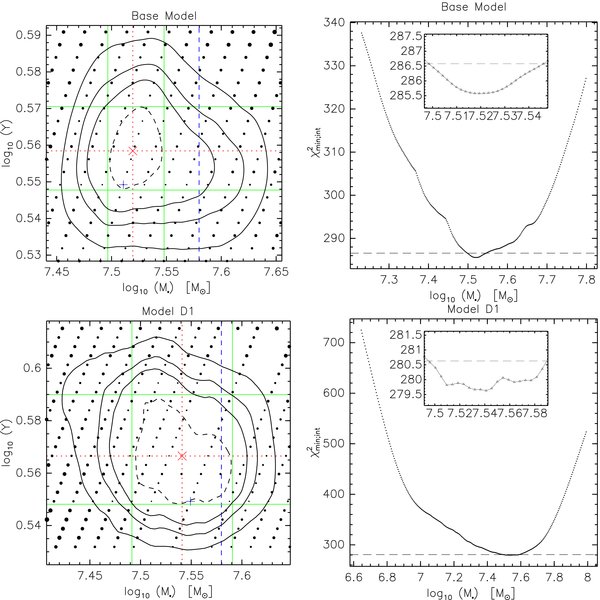
The results from the dynamical modeling are summarized in Table 4, and the corresponding χ2 contour maps are shown in Figure 14. The black hole mass for the base model, which uses the V-band profile without the central peak for both the mass and the kinematic tracer profiles, is M• = 3.31+0.22−0.17 × 10⁷ M☉, with a total (not per degree of freedom) χ2min ≈ 290. The internal velocity moments of the base model are illustrated in Figure 15.
Download figure:
Standard image High-resolution image
Download figure:
Standard image High-resolution image
Download figure:
Standard image High-resolution image
Download figure:
Standard image High-resolution image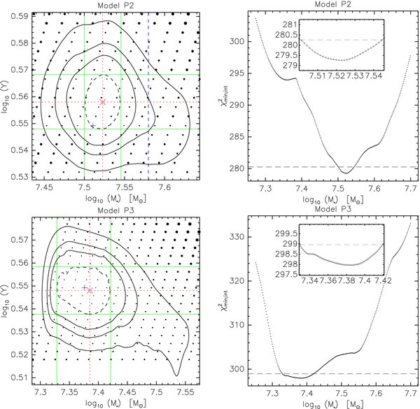
Download figure:
Standard image High-resolution image
Figure 14. Left: contour maps of χ2(M•, ϒ) for the dynamical models bearing the parameters listed in Table 4. Model names are as in Table 4. The stellar M/L ratio (ϒ) refers to the V band. Each dot represents a model, and dot size is proportional to the value of χ2 for that model. The symbol "+" corresponds to the "best" model (χ2min). The symbol "X" corresponds to the minimum interpolated χ2. The contour levels are drawn for Δχ2 ≡ χ2 − χ2min;int = 1.0 (dashed), 2.71, 4.0, and 6.63, corresponding to confidence levels of 68%, 90%, 95%, and 99%, respectively, for one degree of freedom. The horizontal and vertical solid lines indicate the nominal "1σ" one-dimensional uncertainties. The vertical dashed line indicates the maser mass. Right: values of χ2min;int marginalized over the ϒ axis. The horizontal dashed line indicates the Δχ2 = 1 level.
Download figure:
Standard image High-resolution image
Figure 15. Internal moments of the baseline model in the equatorial plane. The red line illustrates the mean rotational velocity 〈vϕ〉 and the dotted line is the velocity dispersion in the ϕ direction  . The solid line is the radial dispersion σr and the dashed line is σθ.
Download figure:
Standard image High-resolution imageTable 4. Dynamical Models
| Model | Massa Profile | Tracera Profile | Kinem.b Data set | ic (°) |  d d |
M•e (107 M☉) | ϒe | Sections |
|---|---|---|---|---|---|---|---|---|
| Base | Vcorr | Vcorr | S+G | 72 | 0.35 | 3.31+0.22−0.17 | 3.6+0.1−0.1 | 5.1 |
| D1 | Vcorr | Vcorr | S+G | 72 | 0.45 | 3.48+0.42−0.38 | 3.7+0.2−0.2 | 5.2.1 |
| D2 | Vcorr | Vcorr | S+G | 62 | 0.35 | 3.62+0.38−0.49 | 3.8+0.1−0.2 | 5.2.2 |
| K1 | Vcorr | Vcorr | S1 + G | 72 | 0.35 | 3.25+0.21−0.13 | 3.6+0.1−0.1 | 5.3 |
| K2 | Vcorr | Vcorr | S3 + G | 72 | 0.35 | 2.20+0.54−0.31 | 3.6+0.1−0.1 | 5.3 |
| K3 | Vcorr | Vcorr | G | 72 | 0.35 | 1.03+1.00−0.28 | 3.7+0.1−0.2 | 5.3 |
| K4 | Vcorr | Vcorr | S+G1 | 72 | 0.35 | 3.33+0.21−0.19 | 3.7+0.1−0.1 | 5.3 |
| P1 | NIRcorr | Vcorr | S+G | 72 | 0.35 | 2.49+0.09−0.10 | 3.5+0.1−0.1 | 5.4 |
| P2 | Vcorr | NIRcorr | S+G | 72 | 0.35 | 3.33+0.18−0.17 | 3.6+0.1−0.1 | 5.4 |
| P3 | NIRcorr | NIRcorr | S+G | 72 | 0.35 | 2.43+0.21−0.30 | 3.5+0.1−0.1 | 5.4 |
| P4 | V | V | S+G | 72 | 0.35 | 3.25+0.22−0.14 | 3.6+0.1−0.1 | 5.4 |
Notes. aMass and tracer profiles named as in Figure 12 (see Section 5.4). bS = All STIS kinematic data listed in Table 3. S1 = As in S but without the central kinematic datapoint.S3 = As in S but without the three central kinematic datapoints. G = All ground-based (Modspec) kinematic data listed in Table 3. G1 = As in G but without the central minor-axis datapoint. cDisk inclination (see Section 5.2.2). Edge-on corresponds to i = 90°. dIsophote ellipticity, assumed constant throughout the galaxy (see Section 5.2.1). eBlack hole mass and stellar M/L ratio (ϒ), assumed constant throughout the galaxy (see Section 5.1). Uncertainty values correspond to the nominal "1σ" one-dimensional uncertainties from the contour maps (Figure 14). The M/L ratio calibration is in the V band.
Download table as: ASCIITypeset image
The total number of parameters is 27 (LOSVDs) times 13 (velocity bins), which is 351. Typically, the reduced χ2 is 0.3–0.5 in our models (Gebhardt et al. 2003), which is less than the expected value of unity because of covariance in the LOSVD components. For NGC 4258, the reduced χ2 is near unity, but most of the contribution to χ2 comes from the minor axis. The velocity centroid on the minor axis varies much more than the stated uncertainties (see Figure 11), whereas an axisymmetric model would have zero velocity along the minor axis. Regardless of whether this contribution is due to underestimated uncertainties or real nonaxisymmetric motion, it is the main cause for the inflated χ2. Along the major axis, the reduced χ2 is about 0.4, which is typical for the orbit-based models.
5.2. Ambiguities in the Deprojection Parameters
5.2.1. Isophotal Ellipticity ()
The (projected) ellipticity profile of NGC 4258 is discussed in Section 3. The profile varies with radius, but the origin of the variation (disk, weak bar, genuine variations in the axis ratios of the bulge isodensity spheroids) is not clear. Therefore, although it is possible to incorporate an arbitrary ellipticity profile (r) in our modeling algorithm, we preferred instead to make models with a constant ellipticity profile, and examine the extent to which M• is affected by the adopted value.
For the base model, we used = 0.35, corresponding to the mean ellipticity in the radial range 2'' ≲ r ≲ 65''. The effect of varying was examined in model D1, for which we used = 0.45. We obtained M• = 3.48+0.42−0.38 × 10⁷ M☉, a slightly higher mass but within the same "1σ" confidence as the base model.
Nonetheless, the assumption of constant ellipticity is clearly problematic because the ellipticity profile varies between ∼0.1 and ∼0.6.
5.2.2. Disk Inclination Angle (i)
We need to know the inclination of the disk to deduce the intrinsic ellipticity of the isophotes from their projected ellipticity, under the assumption that the equatorial plane of the bulge of the galaxy is coplanar with the galactic disk.
The outer disk (beyond r ≈ 200'') has average and maximum ellipticities of = 0.62 and 0.64, respectively. If this disk is infinitesimally thin, the corresponding inclination angles are i = 69° and 70°, respectively, where edge-on corresponds to i = 90°. If this disk were thick with an intrinsic axis ratio of 0.25 (Sandage et al. 1970), then the corresponding inclinations would be i = 73° and 75°, respectively. At large radii, the optical PA is 150°. van Albada (1980), using H i kinematic observations, derives the same PA and i = 72°, which is consistent with the photometrically derived inclination given the uncertainty in the intrinsic thickness of the disk.
We, therefore, adopted i = 72° for the base model, but we also examined the sensitivity of M• to variations in i. Model D2 is identical to the base model except i = 62°, a value close to the lowest inclination angles that we found in the literature. We obtained a ∼10% higher mass, M• = 3.62+0.38−0.49 × 10⁷M☉, which is consistent with a M• ∝ (sin i)−1 dependence. This would be expected in a rotationally supported system. It appears from our models that the inner part of the galaxy is rotating quite rapidly. For this model, χ2min = 303, which is greater than 280, the χ2min for the base model. This could be interpreted as evidence that the base model is more likely to be true, at least within the framework of assumptions of the modeling method.
We did not attempt to obtain a better estimate for the errors due to deprojection (by running models for more combinations or i and ), because the uncertainties in the luminosity profiles (Section 5.4) dominate the errors.
5.3. Ambiguities in the Kinematic Data
In Section 2.2, we mentioned that the presence of an emission line near the CaT in the nuclear STIS spectrum may have affected the reliability of the LOSVD extraction. In fact, the next two STIS spectra (at R = 0 05 and 0''10) show (weaker) signatures of the same emission line, as well. We also mentioned that we have some concerns about the quality of the central LOSVD along the minor axis in the ground-based data. In this section, we remove the suspect LOSVDs from the χ2 fit, and examine the effect on M•.
In models K1 and K2, we isolate the uncertainty introduced to M• by the potentially unreliable LOSVD extraction. Model K1 is identical to the base model, except the nuclear STIS LOSVD is not included as a constraint. In model K2, the three innermost STIS LOSVDs are not included. In model K1, the effect on M• is very small. This is reassuring, since it is the nuclear spectrum that would have been affected the most. Model K2 yields a significantly lower M• = 2.20+0.54−0.31 × 10⁷ M☉ but with a much higher uncertainty, which overlaps with the base model at the ∼1.5σ level.
An interesting question is whether HST spectroscopy is required to find evidence for a black hole. Using ground-based kinematic data alone should, of course, yield a black hole mass consistent with the mass obtained by also including HST data, albeit with larger uncertainties, depending primarily on the angular size of the radius of influence of the black hole on the sky. We address this question for NGC 4258 with model K3, which is identical to the base model, except only ground-based kinematic data are used. It turns out that the stellar M/L ratio can be constrained quite well, but the black hole mass, M• = 1.03+1.00−0.28 × 10⁷ M☉, is very uncertain. This is not surprising, considering that the radius of influence for the black hole in the base model is GM•/σ2e ≈ 0 32, where σe = 105 km s−1 is the velocity dispersion in the main body of the bulge. This is substantially smaller than the spatial resolution of the ground-based kinematic data, for which FWHM = 1''–15. Therefore, HST kinematic data are critical for a well constrained estimate of the black hole mass in this galaxy. HST photometric data are also critical for galaxies where the luminosity profile near the center cannot be reliably extrapolated from the profile farther out, as is also the case with this galaxy (unfortunately, it is still not possible to determine unambiguously the inner mass profile, as discussed in Section 5.4).
We also constructed model K4, which uses all kinematic data (STIS+Modspec) except the central ground-based LOSVD along the minor axis (the central ground-based LOSVD along the major axis was not included in any model). We find that M• is essentially identical to that of the base model.
5.4. Ambiguities in the Mass and Kinematic Tracer Profiles
In Section 4, we saw that stellar population gradients and/or dust extinction in the innermost ∼2'' of the galaxy, as well as light from the unresolved AGN, can induce variations in the measured stellar M/L ratio near the center of the galaxy. These have to be taken into account to determine which, if any, of the available luminosity profiles traces the mass–density profile, and which, if any, corresponds to the luminosity profile of the kinematic tracer population. The latter profile is needed for the luminosity weighting (normalization) of the LOSVDs. Unfortunately, we were unable to make these determinations convincingly, for the reasons explained in Section 4.
Consequently, we decided to identify three possible luminosity profiles, and to make models that use them as either mass or kinematic tracer profiles. The expectation is that these three profiles correspond to limiting cases, and that the true profiles lie somewhere in between. Then, the spread in M• that we obtain from these limiting cases would be a good indication of the M• uncertainty caused by our inability to determine the true profiles.
The profiles, which are depicted in Figure 12, are the following.
- 1.The V profile. This is identical to the V-band profile as measured.
- 2.The Vcorr profile. This is identical to the V profile, with the three innermost points replaced by a shallower core, as explained in Section 4.2.
- 3.
If the observed color gradient is mostly or entirely due to the presence of diffuse dust or metallicity, then the NIRcorr profile is a better tracer of mass than the V or the Vcorr profiles. However, the V-band profile has higher intrinsic resolution and a dimmer AGN, and the WFPC2 is better understood photometrically than NICMOS. For these reasons, we try all three versions as stellar mass profiles.
The kinematic tracer population was observed in the CaT wavelength, which lies in the I band. It would, thus, be natural to use the I-band profile as the kinematic tracer profile. However, we saw in Section 2.1.2 that the I-band image is saturated in the central 009, and thus cannot be deconvolved. The NIR profile shares the same slope with the I-band profile at larger radii (where I is not saturated), and could arguably be used instead. Unfortunately, it is also ill determined near the center due to the AGN and reduced resolution (Section 4.1). Consequently, we decided to again test both NIRcorr and Vcorr as the kinematic tracer profile, and examine the induced uncertainty in M•. For the base model, we adopted Vcorr because of its higher resolution and smaller AGN contamination. This is somewhat arbitrary, but the choice of the kinematic tracer profile turns out to have a very small effect on M•, as we will see below.
These scenarios were tested in models P1 through P4. Models P1–P3 substitute NIRcorr for Vcorr in the mass and/or kinematic tracer profiles, and show that the choice of the stellar mass profile matters much more than the choice of the tracer profile. When Vcorr is used for the mass profile (base model and P2), M• = 3.31+0.22−0.17 × 10⁷ M☉ or M• = 3.33+0.18−0.17 × 10⁷ M☉, depending on whether Vcorr or NIRcorr is used, respectively, for the tracer profile. These numbers become 2.49+0.09−0.10 × 10⁷M☉ and 2.43+0.21−0.30 × 10⁷ M☉, respectively, when NIRcorr is used for the mass profile (models P1 and P3). The relative insensitivity to the choice of the tracer profile is not surprising, considering that, e.g., for a spherical system, the tracer profile ν(r) affects mass M(r) within the radius r only via dln ν/dln r, which by construction is nearly identical for both Vcorr and NIRcorr near the center of the galaxy.
Model P4 substitutes V for Vcorr in the mass profile. It yields M• = 3.25+0.22−0.14 × 10⁷ M☉, very similar to the base model, reflecting the fact that the only difference between P4 and the base model is the small luminosity excess within 004 of the nucleus, well below the spatial resolution of the kinematic data (∼01). The stellar M/L ratio is constrained at larger radii, so that the only difference in the stellar mass profile, M*(r), between P4 and the base model is due to this small luminosity excess. From the M• − M*(r0) degeneracy, discussed in Section 4.2, the only option for the modeling algorithm is to reduce M• by a (small) amount equal to the difference in stellar mass inside r0 ≈ 0 1 between P4 and the base model.
This point is illustrated in Figure 16, which shows the stellar mass profile, M*(r), and the total mass profile, M• + M*(r), for the base model and for models P1 and P4. The mass profiles of these models correspond to the three profile choices (Vcorr, NIRcorr, and V, respectively) discussed above. It is clear that dynamic modeling assigns black hole masses to P4 and to the base model such that they both contain the same total mass inside r ≃ 0 04 (since both models are constrained by the same kinematic data and the same V-band mass profile beyond r ≃ 0 04). This is not the case with model P1 which, although again constrained by the same kinematic data set, is characterized by a different mass profile (NIRcorr) outside of ∼0 1, the spatial resolution of the kinematic data.
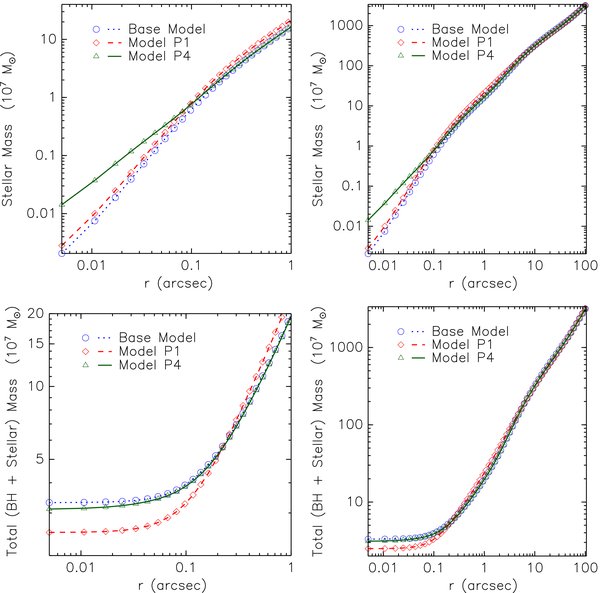
Figure 16. Enclosed stellar mass M* (top row), and sum of the black hole mass and the enclosed stellar mass M• + M* (bottom row), as a function of model radius. The base model and model P4 are constrained by the same kinematic data set, and they share the same mass V-band profile for r > 0 04 (see Table 4). Because of the degeneracy between M• and M* within a small radius r0 ≈ 0 1 from the center, comparable to the spatial resolution of the kinematic data, the modeling algorithm can only constrain the total mass inside that radius. As a result, model P4 is assigned a slightly lower M• to compensate for the excess mass contained in the central "bump" of its mass profile. Model P1 is characterized by the NIRcorr mass profile, which differs from that of both P4 and the base model at r > r0.
Download figure:
Standard image High-resolution image6. DISCUSSION
The determination of the central black hole mass in NGC 4258 from stellar dynamics proved tougher than anticipated. The main source of difficulty (and uncertainty in M•) comes from the presence of a V − J color gradient in the central ∼2'' of the galaxy, which prevents us from determining the stellar mass profile near the center with confidence. The model that we trust most ("base model" in Table 4) yields M• = 3.31+0.22−0.17 × 10⁷ M☉ and assumes that the stellar mass is traced by the "corrected" V-band profile, or Vcorr (Figure 12). This is identical to the V-band profile except for the removal of a small luminous "bump" in the central ∼004, which we attribute to the AGN. Using the uncorrected V-band profile yields a very similar M• = 3.25+0.22−0.14 × 10⁷ M☉ (model P4 in Table 4). This small black hole mass "deficit," compared to the base model, corresponds approximately to the mass of stars in the luminosity "bump" and is a consequence of the degeneracy between stellar mass and black hole mass very near the center (Section 4.2; Figure 16).
Using the steeper J-band (NIR) profile as the mass tracer (model P1), we obtain M• = 2.49+0.09−0.10 × 10⁷ M☉, a factor of 25% lower than in the base case. Although V-band light is more likely to be compromised as an indicator of the stellar mass distribution than J-band light, due to extinction and metallicity gradients, we have greater confidence in the base model because (1) the V-band profile is better determined near the center owing to the higher resolution of the V images, (2) the AGN is considerably fainter in V than in J, making it easier to subtract, and (3) the minimum χ2 for the base model is 280, significantly less than the minimum χ2 for the P1 model using J-band data (which was 303).
The spread in M• introduced by uncertainties in the deprojection parameters (models D1 and D2) is only of order 10%, so it is the uncertainties in the stellar mass profile that dominate the errors.
After all these sources of error are taken into account, our black hole mass determination is ∼15% lower than the "preferred" maser determination [(3.82 ± 0.01) × 107 M☉] and only 7% lower than the lowest maser determination [(3.59 ± 0.01) × 107M☉] (rescaled to our distance for the galaxy). We view this level of agreement (2σ) as evidence that stellar-dynamical mass determinations using similar methods to those in this paper, and with data of comparable quality, are accurate at the 2σ level or better. Our previous work has sought to avoid galaxies with dusty centers such as NGC 4258. In this case, obscuration of high-velocity stars by the compact nuclear dust patch (Section 2.1.2), possibly associated with the masing disk, could be responsible for an underestimate of the black hole mass in our work. To these problems should be added possible systematic effects due to deviations from axisymmetry, which cannot be properly treated by our axisymmetric modeling code. We also note that the discrepancy between the mass determination from stellar dynamics and the maser mass determination in NGC 4258 is smaller than the discrepancy between the stellar-dynamical mass determination and the mass determination from individual orbits for our own Galaxy, which amounts to about a factor of 2 (Chakrabarty & Saha 2001; Ghez et al. 2005). Most concerns about black hole mass estimates from stellar dynamics have stressed the likelihood that the masses are overestimated, whereas here the stellar-dynamical mass is smaller than the maser mass.
Finally, although we regard the maser mass in NGC 4258 as the gold standard in black hole masses, it is conceivable, however unlikely, that some unrecognized effect has led to an overestimate of the mass determined from maser kinematics.
We are grateful to Eric Becklin and Ranga Chary for providing the HST NICMOS images, and to Tom Jarrett for providing the 2MASS images before publication. We thank the referee, Tim de Zeeuw, for comments that improved the manuscript. C.S. is grateful to Seppo Laine and Ranga Chary for useful discussions. Support for proposal GO–8591 was provided by the National Aeronautics and Space Administration (NASA) through a grant from the Space Telescope Science Institute, which is operated by the Association of Universities for Research in Astronomy, Inc., under NASA contract NAS 5-26555. Support for this research was also provided by NASA grant NAG 5-8238 to the University of Michigan. A.V.F. is grateful for the support of NSF grant AST–0607485. This research has made use of the NASA/IPAC Extragalactic Database (NED) which is operated by the Jet Propulsion Laboratory, California Institute of Technology, under contract with NASA.
APPENDIX: DESCRIPTION OF THE ORBIT-SUPERPOSITION METHOD
For over two decades, orbit-superposition methods have been used to study the dynamics of galaxies. Originally invented to construct a model of a triaxial galaxy (Schwarzschild 1979), the methods have become the tool of choice for interpreting data in terms of equilibrium galaxy models. The most important feature of orbit-superposition methods is that they provide a constructive proof that a given set of photometric and kinematic data can (or cannot) be reproduced by an equilibrium stellar system in a specified gravitational field. The computer code described in this appendix has been used to estimate black hole masses in galaxies (Gebhardt et al. 2003) and to determine the relative contributions of dark and luminous matter in elliptical galaxies (Thomas et al. 2004, 2005). It is a descendant of the spherical program described in Richstone & Tremaine (1988), but improved in two major respects: it treats the galaxy as axisymmetric rather than spherical, and it matches the full LOSVD of the galaxy at specified positions on the sky, rather than the second moment only. Similar programs have been developed by van der Marel et al. (1998); Cretton et al. (1999); Valluri et al. (2004).
A number of preliminary steps must be taken to convert the reduced data into inputs for the orbit-superposition method. These include the deprojection of the observed surface brightness to construct a light distribution in three-dimensional space and the reduction of spectra at different locations on the sky to projected velocity distributions. Both of these activities require additional assumptions or choices. We normally deproject under the assumption that level surfaces in stellar density are coaxial spheroids (Gebhardt et al. 1996), and we normally use a penalized maximum-likelihood estimator to construct the LOSVDs (Gebhardt et al. 2000a; Pinkney et al. 2003). Next we compute the gravitational field from the three-dimensional light distribution under the assumption that the mass consists of a black hole of mass M• and stars having a M/L ratio independent of position. Dark matter can be incorporated into such a model, but we have not done so here.
Once the preliminaries are complete, the calculation of a dynamical model by this method consists of two steps. First, a library of orbits is constructed using initial conditions that cover all possible locations in phase space. Each orbit's contribution to the surface brightness and projected velocities is logged. Second, the orbits are combined to match the light distribution and LOSVDs of the galaxy as well as possible (using χ2 parameter to assess the goodness of fit). This procedure is repeated for a set of black hole masses, and limits on the latter are set from χ2 as a function of M•. Note that although different orbit libraries are required for each different ratio of M/L to M•, a single library can be used for various values of M• so long as M/L scales with M•.
A.1. The Orbit Library
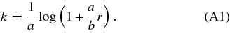
We construct the model on a grid in coordinates r, η, where r is the radius and η is the latitude. We restrict ourselves to potentials (and mass distributions) symmetric about the equator. The grid is evenly spaced in ν = sin (η) from ν = 0 to 1, and in r in even intervals in k defined by
Bins in (r, η) are bounded by the grid points. Below, we also use standard cylindrical coordinates (ϖ, z). It is essential to explore the phase space of orbits with a resolution at least as fine as the resolution used to construct the models.
Orbits in axisymmetric potentials always have two isolating integrals, the energy E, and the z-axis angular momentum Jz. Regardless of the possible presence of a third integral, conservation of E and Jz confine the orbit within a region of (ϖ, z) space defined by a boundary where the orbits' velocities are zero:
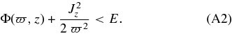
The allowed volume intersects the equator only over a limited range in radius with an upper and a lower limits. We choose (E, Jz) pairs so that there is an orbit with upper and lower limits in the middle of each radial bin. We associate an area with each grid point (ΔE × ΔJz) by halving the distance to adjacent grid points. For each specified (E, Jz), the section of allowed phase space (we ignore ϕ because of the conservation of Jz) that lies on the equator is a two-dimensional surface with coordinates ϖ and vϖ (a surface of section). A regular orbit is defined by a curve on this surface. We systematically tile this surface in the manner invented by Thomas et al. (2004), launching an orbit from the center of each bin and assigning a phase-space volume to each orbit by
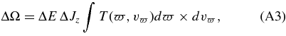
based on the work of Binney et al. (1985), where T is the time between successive crossings of the equatorial plane.
The procedure above gives a starting position for each orbit in the equatorial plane of the model with a well defined ϖ, vϖ, E, and Jz. We use E to determine vz, and we integrate the motion of the orbit in the (ϖ, z) plane. Assuming that all orbits cross the equator, it is a complete survey of orbits. We follow the orbits of stars in spherical coordinates to take advantage of the near sphericity of the mass distribution in the region where a black hole may dominate the gravitational field. Using r as the radial coordinate, η as the equatorial angle, and ϕ as the axial angle, the equations of motion are
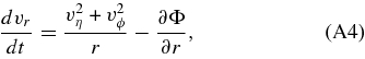
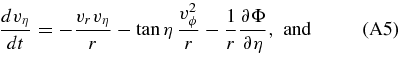
The first two equations are integrated using a standard fourth-order Runge–Kutta method with variable time step, and vϕ is recovered at each time step from Equation (A6). We obtained good energy conservation by letting dt = r/vcirc(r), where vcirc is the velocity of a circular orbit at that radius, with between 0.01 and 0.1. Orbits are followed for about 100 crossing times. We terminate the calculation of an orbit if its energy error exceeds 1%. Typical energy errors are 0.1%. The potential is set equal to zero at ∞.
The accelerations for the orbit integrations are determined by decomposing the assumed galaxy density distribution in spherical harmonics. Specializing immediately to axisymmetry gives
with
and where ν = sin η. The gravitational acceleration on the orbit is determined by differentiating Equation (A7) with respect to r and η.
We tested our expansion in a Kuzmin–Kutusov model (Dejonghe & de Zeeuw 1988) with a/c = 0.5, which corresponds to a very flat galaxy (about E5). This model has analytical density, potential, and accelerations. Truncating the expansion at P6 accurately reproduces the exact accelerations to 1% or better everywhere in the galaxy, so we set lmax = 6 in Equation (A7).
The additional acceleration from a mass point is straightforward to add to the radial component of the accelerations above. We store and model the galaxy in the angular range 0° ⩽ η ⩽ 90°. We store the three lowest order internal moments in each bin for each orbit (mass m, mv, mvv) for later use.
Simultaneously, the projected line-of-sight velocities are binned in a three-dimensional grid in projected radius R, angle β (measured from the major axis of the galaxy on the plane perpendicular to the line of sight), and velocity v. The spacing in R and β is defined as above. Since the orbits are being followed in r and η, ϕ is not defined. At each time step, in order to project the orbit onto the line of sight, we choose 100 values of ϕ, evenly spaced from 0 to π.
A.2. Matching the Light Distribution and Observed Dynamics
The next step is to find the superposition of orbits consistent with the stellar mass distribution that best matches the observed LOSVDs. Richstone & Tremaine (1988) provide an efficient method to match the mass distribution that can be augmented to minimize χ2. Their method maximizes an objective function
while satisfying a set of constraints
We choose to maximize the objective function
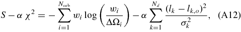
where wi is the weight of the ith orbit and lk is the light in the kth bin in the observational phase space composed of the position on the sky and the line of sight velocity. The more familiar LOSVD is the distribution of light in line of sight velocity at a single position on the sky. Thus, the index k identifies a small range in both projected velocity and projected position. The variable α is an adjustable parameter discussed further below. There are Norb orbits in the orbit library, and k varies from 1 to Nd, where Nd is the number of positions at which the LOSVD has been measured times the number of velocity intervals at each measurement. The first sum in Equation (A12) is an entropy, and the second is a χ2 that measures the goodness of a fit of the model LOSVDs to the observed LOSVDs. The sum of the orbits must also match the deprojected (three-dimensional) light distribution in the Nbin bins:
where mij is the mass contribution of the ith orbit to the jth bin.
In order to put Equation (A12) in the form of Equations (A10) and (A11), we make the following substitutions and identifications. First, we define xi = wi for i = 1, Norb, and add an additional set of variables that measure the error in the light projected into each LOSVD bin  for k = 1, Nd. Since the light in each bin of the model LOSVDs is given by the contribution of each orbit to that projected velocity and position there is an additional set of constraint equations of the form the form
where k = j − Norb, and mij is the contribution of the ith orbit to the kth component of the set of LOSVDs.
Then, we have
defining Ci in Equation (A10), and Equations (A13) and (A14) correspond to Equation (A11). Note that for i > Norb, −Ci is maximized at xi = 0. The first set of Ci (for i ⩽ Norb) effectively keeps the orbit's weight positive. The second set (for i > Norb) minimizes the components of χ2. We then use the method described by Richstone & Tremaine (1988) to iteratively solve the equations.
An important feature of this problem is the choice of the parameter α. Although we have not devised a method to specify appropriate values of this parameter in advance, if the quantity χ2 reflects a satisfactory accounting of the estimates of errors in the recovery of the LOSVDs of the target galaxy, then the choice of α and interpretation of the results are reasonably straightforward. A small α will generally produce a solution. Increasing α slowly decreases χ2, but not beyond some limit. In practice, we start with α = 0 and increase it slowly until the change in χ2 is less than 0.02 in a single iteration.
A.3. A Test with a Black Hole
In this case, we specify a dynamical model with a gravitational potential and a distribution function (DF) for the stars (the starlight need not, and does not, determine the mass in this model). The gravitational potential is
This potential includes a point mass and a flat circular velocity curve (with velocity vcirc) at large r. We investigated Michie-like DFs of the form
where A is normalization, E and Jz are energy and angular momentum, wϖa (an anisotropy distance), N, and σ (a velocity dispersionlike quantity) are model parameters, and E1 and E2 are upper and lower limits of the energy. The function ⊓ is defined by
The DF can be rewritten as
where t2 = v2ϖ + v2z,  and
and  . This function has a number of interesting properties: N > 0 tends to create vϕ enhanced anisotropy and a flattened density distribution;
  tends to depress vϕ and creates a prolate density distribution. The cutoffs in energy avert a divergence in the luminous matter distribution near the black hole.
The density is
where t2 = v22 − v2ϕ and t1 = max(v21 − v2ϕ, 0).
Note that the distribution functions with different choices of parameters can be added to each other (in the same potential), and similarly the densities and density-weighted moments are additive. A Monte Carlo realization of the model is constructed by sampling each density distribution and choosing the velocities randomly from the velocity distribution. Note that we have the additional freedom of choosing an arbitrary fraction of the ϕ velocities in the positive sense, and hence setting the spin of any model between a maximum amount and zero. The total number of random variates chosen sets the normalization.
For the test here, we adopted a potential with vcirc = 220 kms−1 and M• = 1.126 × 10⁸ M☉. We added two DFs. The first had σ = 160 kms−1, ϖa = 600 , N = 0, E1 = Φ(10 ), E2 = Φ(1000 ), with equal numbers of the ϕ velocities chosen in the positive and negative sense. The second DF had σ = 120 kms−1, wa = 200 , N = 2, E1 = 10 , E2 = 1000 and 3/4 of the ϕ velocities were chosen positive. Each DF was assigned 1/2 × 109 random points, so they had equal mass. The second DF, featuring a moderately spinning disky structure, dominates the model near the center of the galaxy, but declines rapidly. The first DF, a mildly prolate structure with no net spin dominates further out. No stars are found beyond a radius of 1000 from the center of the model. The 109 random points each are converted to projected positions and velocities (we assumed the galaxy was edge on), and binned into "observations" mimicing our combined HST and ground-based data, and also producing data mimicing data that would be obtained with an integral field unit. For the example, below we used the IFU data with a resolution of 10 at the center, and lower resolution data extending to a distance of 800 from the center. At each location, the projected velocity variates were binned at a resolution of 20 kms−1. Gaussian noise was added to the data in a series of 20 realizations. These data sets were then fed into the modeling program, which produced (in each case) a χ2 map in vcirc and M•.
Marginalizing over each variable, in turn, produced the determinations of M• and vcirc illustrated in Figure 17. Each data set had LOSVDs at 32 positions with 15 velocity bins, a product of 480. For each realization of this set, the best-fit model had a χ2 near 500. Since the velocity bins are uncorrelated in these data sets, this is about the expected χ2. For the presentation in Figure 17, the plots of χ2 against black hole mass and vcirc were arbitrarily shifted to a minimum of 500. The error bars judged from the individual χ2 profiles are about 20% smaller than the error (above) determined from the spread in minima. The mean values of M• and vcirc from these experiments were (1.15 ± 0.03) × 108 M☉ and 222 ± 5 kms−1, in excellent agreement with the target values.
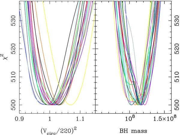
Figure 17. χ2 profiles of orbit-based models of the Monte Carlo model described in Appendix A.3. The left panel illustrates the recovery of the circular velocity of the potential for 20 different realizations of its LOSVDs. The right panel illustrates the recovery of the black hole mass from the same set of realizations. The plots in each panel are marginalized over the variable in the other panel. The mean of the derived black hole masses is 1.15 × 10⁸ M☉, consistent with the model mass.
Download figure:
Standard image High-resolution image
An earlier version of the code suffered from a units conversion error that led to an underestimate of black hole masses (and M/L). All black hole masses obtained with this program published in or prior to 2003 should be multiplied by 1.09.
Footnotes
- 14
Throughout the paper, R refers to distance from the center of the galaxy, while r refers to distance along the isophotal semimajor axis.