


ABSTRACT
We present the first comprehensive examination of the geysering, tidal stresses, and anomalous thermal emission across the south pole of Enceladus and discuss the implications for the moon's thermal history and interior structure. A 6.5 yr survey of the moon's south polar terrain (SPT) by the Cassini imaging experiment has located ∼100 jets or geysers erupting from four prominent fractures crossing the region. Comparing these results with predictions of diurnally varying tidal stresses and with Cassini low resolution thermal maps shows that all three phenomena are spatially correlated. The coincidence of individual jets with very small (∼10 m) hot spots detected in high resolution Cassini VIMS data strongly suggests that the heat accompanying the geysers is not produced by shearing in the upper brittle layer but rather is transported, in the form of latent heat, from a sub-ice-shell sea of liquid water, with vapor condensing on the near-surface walls of the fractures. Normal stresses modulate the geysering activity, as shown in the accompanying paper; we demonstrate here they are capable of opening water-filled cracks all the way down to the sea. If Enceladus' eccentricity and heat production are in steady state today, the currently erupting material and anomalous heat must have been produced in an earlier epoch. If regional tidal heating is occurring today, it may be responsible for some of the erupting water and heat. Future Cassini observations may settle the question.
Export citation and abstract BibTeX RIS
1. INTRODUCTION
The geysering activity at the high southern latitudes of Enceladus has been a focus of the Cassini Imaging Science Subsystem (ISS) investigation ever since it was first sighted in images taken in early 2005 (Porco et al. 2006). Dozens of distinct, narrow jets, visible only at high solar phase angle, have since been seen erupting from four prominent fractures, dubbed "tiger stripes," straddling the moon's south polar terrain (SPT)3. These eruptions consist of two components: solids, in the form of micron-sized water ice particles (Porco et al. 2006; Spahn et al. 2006; Hedman et al. 2009) and vapor (Hansen et al. 2006; Waite et al. 2009; Hansen et al. 2011).
The total mass flux in the solid component, deduced from the analysis of very low resolution ISS images of the spatially integrated plume formed by the jets, is 51 ± 18 kg s−1 (Ingersoll & Ewald 2011). The Ultraviolet Imaging Spectrometer (UVIS) measured a total mass flux in vapor of 200 kg s−1 coming from the entire SPT, with only ∼4% in the form of jets (Hansen et al. 2011). Consequently, the ratio of the mass flux in solids to the total vapor mass flux is roughly 0.3 ± 0.1, and clearly larger than the ∼0.01–0.05 expected if the jet particles were produced by the expansion, adiabatic cooling, and direct condensation of vapor to solids (Schmidt et al. 2008; Ingersoll & Pankine 2010). This argument was used early in the mission to suggest a liquid water source for the jet particles (Porco et al. 2006; Ingersoll & Ewald 2011). A more appropriate comparison, however, is the solid/vapor ratio in the jets alone; this ratio is ∼6, significantly strengthening the conclusion that the source of most of the solids in the jets is liquid water, or, in other words, that the jets are the Enceladus equivalent of geysers. (Throughout this paper, we use the terms "jets" and "geysers" interchangeably.)
The vapor sampled by the Cassini Ion and Neutral Mass Spectrometer includes predominantly water with trace amounts of ammonia, carbon dioxide, and methane, as well as various species of light hydrocarbons (Waite et al. 2009). A full 99% of the mass in the jets' solid component is salt-rich, with salinity between 0.5% and 2%—comparable to that of the Earth's ocean, and in marked contrast to grains collected in the E ring, which are on average salt-poor (Postberg et al. 2011). The abundance of salt in the near-surface particle component, the lack of Na in the near-surface vapor (Waite et al. 2009) and in the E ring (Schneider et al. 2009), the fact that most of the particles fall back to the surface (Porco et al. 2006; Ingersoll and Ewald 2011), and the presence of a vertical stratification in particle size with the largest being closer to the surface (Schmidt et al. 2008; Hedman et al. 2009), strongly suggest that the largest near-surface particles are salt-rich and are frozen droplets of salty liquid water. The most likely source of this water is a global ocean or regional sea sitting directly above a rocky core. The salt-poor particles in the E ring are likely the result of the condensation of relatively salt-free plume vapor (Postberg et al. 2011).
Analysis of medium to low resolution images of the jets spanning the early years of the Cassini mission, from late 2005 to early 2007 (Spitale & Porco 2007), revealed a spatial coincidence between four of the eight most prominent jet features observed by ISS on the tiger stripe fractures and surface hot spots observed in 2005 by the Cassini long wavelength infrared spectrometer (CIRS) in low resolution scans of the SPT (Spencer et al. 2006).
Since 2005, several medium and high resolution thermal scans of the SPT and select regions on the tiger stripes have been made by Cassini infrared instruments. Initial analysis of the thermal data acquired by CIRS in 2008 found at least 15.8 ± 3.1 GW of thermal emission from the tiger stripes (Howett et al. 2011). While this value has since been revised down to ∼5 GW (Spencer et al. 2013), the fractures are still the warmest places on the SPT by far. In addition, the high resolution observations made by CIRS and the Visual and Infrared Mapping Spectrometer (VIMS) on Baghdad Sulcus uncovered very small-scale (tens of meters) hot spots on Baghdad Sulcus (Blackburn et al. 2012; Spencer et al. 2012; Goguen et al. 2013). Modeled temperatures of these spots approach 200K (e.g., Goguen et al. 2013).
The mechanism responsible for such a prodigious heat output has come under close scrutiny. The only plausible source of heat is localized tidal deformation and energy dissipation arising from a 2:1 orbital resonance between Enceladus and Dione that maintains the former's eccentric orbit and allows the tidal distortion raised on Enceladus by Saturn to vary in magnitude and direction over an orbit. These diurnal variations produce cyclical patterns of stress on its surface similar to those studied on Europa (Melosh 1977; Hoppa et al. 1999). Over Enceladus' orbital period of 1.3 days, horizontal stresses at any one locale on the fractures will alternate from compressive to shear to tensile, and back again, in principle opening and closing the fractures and producing shear heating in between. A subsurface liquid layer has the decided advantage of enhancing these tidal stresses, and hence flexure in an ice shell overlying the liquid body, and many models addressing different aspects of Enceladus' interior and shape have assumed one.
A global subsurface ocean is difficult to maintain indefinitely. For the present-day eccentricity, and assuming no heating in the core, a global ocean would freeze out on timescales of a few tens of millions of years (Roberts & Nimmo 2008). However, numerical models (Behounkova et al. 2012) show that, in some evolutionary scenarios, a regional subsurface sea can be maintained indefinitely. Survival of a regional as opposed to a global body of water is also more readily reconciled with the long-term averaged tidal dissipation rate, which does not exceed 1.1 GW based on conventional estimates of Saturn's dissipation (Meyer & Wisdom 2007).
Thus, any liquid body today may be restricted to a region no larger than the southern hemisphere (180° across) or smaller, perhaps only 120° across (Tobie et al. 2008), a result consistent with the suggestion (Collins & Goodman 2007) that a localized sea beneath the SPT produces the present-day ∼0.5 km topographic depression seen in Cassini ISS images (Porco et al. 2006; Thomas et al. 2007). Moreover, Doppler tracking of the Cassini spacecraft during three close flybys of Enceladus in 2010 April, 2010 November, and 2012 May has yielded estimates of the dimensionless polar moment of inertia of ∼0.335 and a largely compensated ice shell with a thickness of 30–40 km (Iess et al. 2014). These results suggest a liquid layer at depth but cannot distinguish between a global ocean and a regional sea. However, taken together with the 0.5 km south polar depression and the energetic constraints, the most likely situation is a spatially limited sea of liquid water, roughly 10 km thick and lying beneath a 30–40 km thick ice shell, though a global water layer (which is thicker at the south pole) is not ruled out.
These and other Cassini results and theoretical models make a subsurface lens of liquid water beneath the SPT virtually certain. Additionally, the presence of organic and nitrogen-bearing compounds within this body of liquid water, in contact with a rocky core—all the hallmarks of an extraterrestrial habitable zone—from which issue surface geysers readily sampled by passing spacecraft, make Enceladus an extraordinarily promising body for astrobiological investigation.
Consequently the remaining questions concerning the activity observed at the south pole are pressing: What are the sources of the eruptive material and the heat, and the mechanisms for producing them? In particular, is the source of material composing the jets in the near-surface region or in the sea below? And how is the heat emitted today partitioned between bulk viscous heating currently ongoing under the SPT, cyclical shear (frictional) heating along the opposing fault planes forming the fractures, and emission from already warm material advected from below and/or heat conducted from depth? Finally, what do the answers to these questions imply about the thermal history of Enceladus, and how long it might have been, or continue to be, active?
The CIRS thermal measurements indicate that the vast majority of Enceladus' observed heat is emitted from the tiger stripe fractures (Spencer et al. 2006; Howett et al. 2011) and present-day shear heating along the fractures was initially proposed as the responsible agent (e.g., Nimmo et al. 2007).4 The jetting activity has been associated with the opening and closing of fractures resulting from the diurnal cycling of normal stresses (Hurford et al. 2007)—a suggestion that has recently received support from the observed time-variability of the plume behavior (Hedman et al. 2013; Nimmo et al. 2014, henceforth Paper 2). The relationships, however, among all three phenomena—tidal stresses, anomalous thermal emission, and jetting—are still unclear. Do the shear stresses and associated frictional heating along the walls of the fractures melt the ice there to form liquid water and vapor which supply the geysers and which in turn are modulated by normal stresses? Or do tidal stresses simply create a deeply rooted system of narrow cracks extending tens of kilometers to the sea below, thereby providing the vertical pathways for sea-derived liquid droplets and water vapor, and the latent heat they carry, to reach the surface? Or is it a bit of both?
We seek to understand the mechanisms of material and heat production and transport to the surface by investigating the relationships between the jet activity, the thermal emission, and the tidal stresses affecting the SPT, and we present here the first high and low resolution comparisons among all three phenomena in the service of that goal. We begin by reporting the results of Cassini's now-completed high resolution imaging survey of the SPT and the determination of the three-dimensional distribution of the jets observed there. At the moment, all the Cassini high resolution imaging sequences of the jets that will ever be taken are in hand and with them, a comprehensive accounting has been made from which an accurate and final map—indeed, a 3D SPT jet model—has been constructed. We examine the spatial relationships between jetting and the thermal emission observed by Cassini, and we compare these results to the spatial distribution of tidal stresses. We also examine here the temporal relationships between the eruption state (on or off) of individual geysers found in our survey and the cycling of normal stresses across the SPT. (In Paper 2, we take the alternate approach and compare the variation in total brightness, and presumably total mass, of the spatially integrated plume above the SPT, formed by all its geysers, with predictions derived from several models describing the phase and variation in magnitude of tidal stresses.) Finally, we discuss the implications of all these results for choosing among different mechanisms for explaining Enceladus' south polar activity.
2. DATA ANALYSIS
Since their discovery in 2005, the unique geological province forming the southern polar cap of Enceladus, and the geysers and thermal anomaly found there, have been major observational targets of the Cassini mission. In particular, imaging sequences were designed and executed that called for repeated high resolution views of the jets from a broad range of azimuthal "look" angles relative to Enceladus' prime meridian, and from a limited range of latitudes that placed, for most imaging sequences, the SPT on the moon's limb as seen from the spacecraft. Figure 1 shows representative images used in this study.

Download figure:
Standard image High-resolution image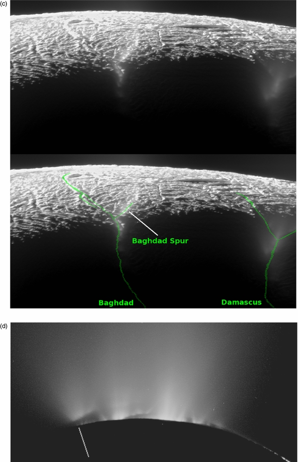
Download figure:
Standard image High-resolution image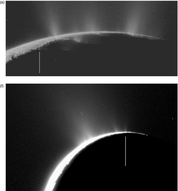
Figure 1. (a) Mosaic of the highest resolution images used in this study. Image scale ∼80 m pixel−1 and a phase angle of ∼145°. (b) Top: an image taken from set BBB at a spatial scale of ∼400 m pixel−1 and a phase angle of ∼163° on 2010 November 30, 1.4 yr after the southern autumnal equinox. The shadow of the body of Enceladus on the lower portions of the jets is clearly seen. Bottom: an ISS image showing the intersection of the shadow of the body of Enceladus with three of the four planes in which the geysers reside. The lines represent the reprojection of Enceladus' shadow on a plane normal to the "top-left" branch of the Cairo fracture (bottom line), normal to the Baghdad fracture (middle line), and normal to the Damascus fracture (upper line). (c) Top: an image from set YY, looking roughly in the direction of Saturn, taken on 2010 August 13, with image scale ∼70 m pixel−1, showing the Saturn-facing ends of Baghdad and its jet-active spur, and Damascus and its split ends. In this set, jets are indistinct and tilts are indeterminate, though their source locations are clearly seen. This set was used for confirmation of source locations triangulated using other images. Bottom: same image with labels. (d) The sole image from set JJJ showing Jet #99, whose location was determined directly by use of the height of the shadow falling on it (Figure 3(b)). (e) The sole image from set XX showing Jet #100, whose location was determined directly by use of the height of the shadow falling on it (Figure 3(b)). (f) An image taken on 2007 September 30 showing Jet #101 seen only in set U. Its source location is indeterminate but the nearly parallel ground tracks derived from two images in this set are shown in Figure 3(b).
Download figure:
Standard image High-resolution imageSuch observations can be used to determine the position and direction of any one jet by the method of triangulation. That is, each jet image yields a line-of-sight "ground track"—a locus of possible surface locations projected onto the surface of the moon. Two images of the same jet from known but well-separated azimuths yield two ground tracks whose intersection gives the surface latitude and longitude of the jet; the closer to α = 90°, where α is the separation angle, the more precise the location determination. With multiple sightings of sufficient angular separation, the position can be further refined; even the tilt of the jet from the zenith may be accurately determined, especially with a separation in azimuths close to 90°. This simple technique was used in analyzing the medium to low resolution images taken early in the mission to ascertain preliminary locations and directions of the most easily identified jets (Spitale & Porco 2007).
We have here superceded that work by utilizing all the useful, high resolution jet images taken by Cassini ISS over the course of the mission—almost all of them acquired since 2007—for the express purpose of surveying the SPT, locating the jets, and creating a 2D map of their surface locations and a 3D model including their tilts. In total, we have reduced 107 images taken from 18 separate observational sequences (each no longer than 3.75 hr but most typically 1–2 hr in duration) comprising a maximum of 25 independent viewing geometries (or "look angles") ranging, by design, over ∼198° in longitude (Figure 2); the observations were taken primarily during close satellite flybys when the spacecraft passed more or less on the side of the moon facing away from Saturn, a result of the inherent design of the Cassini trajectory. The sub-spacecraft latitudes on the moon, from −16 35 to +094, were almost always nearly equatorial; this too was a result of trajectory design and the placement in time of the ISS imaging observations. The images range in pixel scale from 1.34 km pixel−1 to 40 m pixel−1, and in phase angle from 126° to 165°. The identifying names of the 18 observational sets used in this work, the timing, observational characteristics, the number of images within each that was used in this work, and other relevant information are given in Table 1.

Figure 2. Distribution of sub-spacecraft longitudes covered by the 18 imaging sequences used in this study. The observations were taken primarily during close satellite flybys when the spacecraft passed more or less on the side of the moon facing away from Saturn, a result of the inherent design of the Cassini trajectory. The sub-spacecraft latitudes on the moon were almost always near equatorial; this too was a result of trajectory design and the placement in time of the ISS imaging observations.
Download figure:
Standard image High-resolution imageTable 1. Imaging Observation Sets
| Set | Observation Set | Date | Number of | Image Scale | Phase Angle | Sub-s/c | Sub-s/c | Separation | Mean Anomaly | Navigation Procedure |
|---|---|---|---|---|---|---|---|---|---|---|
| ID | Images | [km/px] | (°) | Latitude (°) | W Longitude (°) | α (°) | (°) | |||
| A | ISS_018EN_HIPHAS001_PRIME | 27 Nov. 2005 | 10 | 0.86–0.89 | ∼161.4 | 0.92 to 0.94 | 130.7–138.4 | 0.1–7.7 | 131.1–138.0 | Limb fitting (least-square) |
| U | ISS_050EN_PLUMES001_PRIME | 30 Sep. 2007 | 2 | 1.12–1.19 | 156.5–159.0 | −1.33 to −0.85 | 116.2–117.1 | 0.9 | 289.0–293.1 | Limb fitting (least-square) |
| II | ISS_121EN_ENCEL001_VIMS | 21 Nov. 2009 | 1 | 0.37 | 145.5 | −1.54 | 177.5 | N/A | 126.7 | Manual repointing |
| JJ | ISS_121EN_PLMHR001_PRIME | 21 Nov. 2009 | 9 | 0.04–0.10 | 143.3–145.4 | −14.83 to −6.11 | 194.3–197.3 | 0.2–3.0 | 143.5–147.4 | Limb fitting (least-square) + Tie-points in image N163746187 |
| WW | ISS_136EN_DRKPLUME001_CIRS | 13 Aug. 2010 | 1 | 0.59 | 154.6 | −11.18 | 173.3 | N/A | 26.9 | Limb fitting (least-square) |
| XX | ISS_136EN_PLMHRHP002_PRIME | 13 Aug. 2010 | 8 | 0.18–0.37 | 154.4–154.6 | −16.35 to −12.97 | 186.4–200.3 | 1.5–13.9 | 39.6–52.7 | Limb fitting (least-square) |
| BBB | ISS_141EN_PLMHPHR001_PIE | 30 Nov. 2010 | 6 | 0.39–0.57 | 158.8–162.6 | −0.08 to 0.01 | 288.2–300.4 | 1.2–12.2 | 62.8–79.2 | Tie-points to Enceladus' south polar map |
| CCC | ISS_142EN_PLMHPHR001_PIE | 20 Dec. 2010 | 9 | 0.68–0.91 | 156.1–162.0 | −0.15 to −0.07 | 228.6–275.9 | 3.4–47.3 | 1.1–42.0 | Limb fitting (least-square) |
| DDD | ISS_142EN_NITEMAP001_CIRS | 20 Dec. 2010 | 4 | 0.63–0.64 | 156.7–156.9 | −0.06 to −0.05 | 280.2–281.0 | 0.2–0.8 | 46.9–47.8 | Limb fitting (least-square) |
| EEE | ISS_142EN_PLMHPHR002_PIE | 20 Dec. 2010 | 6 | 0.16–0.31 | 163.3–165.1 | 0.12 to 0.40 | 304.3–314.2 | 1.9–9.9 | 78.3–90.5 | Tie-points to Enceladus' south polar map |
| GGG | ISS_144EN_PLMHPHR002_PIE | 31 Jan. 2011 | 6 | 0.37–0.47 | 126.3–153.5 | −1.25 to −0.97 | 278.5–293.9 | 0.2–15.4 | 95.4–107.7 | Tie-points to Enceladus' south polar map or Manual repointing |
| III | ISS_154EN_PLMHPHR001_PIE | 1 Oct. 2011 | 9 | 0.44–1.23 | 149.6–152.1 | 0.17 to 0.26 | 144.2–178.9 | 2.1–34.7 | 176.7–214.1 | Limb fitting (least-square) and/or Manual repointing |
| JJJ | ISS_155EN_PLMHPHR001_PIE | 19 Oct. 2011 | 9 | 0.60–1.30 | 149.3–152.6 | 0.18 to 0.22 | 141.5–168.9 | 0.5–27.4 | 168.6–199.6 | Limb fitting (least-square) and/or Manual repointing |
| KKK | ISS_156EN_PLMHPHR001_PIE | 5 Nov. 2011 | 6 | 1.03–1.34 | 148.2–149.9 | 0.22 | 140.8–151.6 | 0.4–10.8 | 161.7–174.3 | Limb fitting (least-square) and/or Manual repointing |
| MMM | ISS_161EN_PLMHPMR001_PIE | 20–21 Feb. 2012 | 6 | 0.37–0.64 | 139.4–161.3 | 0.21–0.41 | 127.5–137.2 | 0.1–9.7 | 167.4–183.6 | Limb fitting (least-square) and/or Manual repointing |
| NNN | ISS_163EN_PLMHPHR001_PIE | 27 Mar. 2012 | 7 | 0.71–1.24 | 158.6–160.3 | 0.50–0.52 | 143.6–164.2 | 3.3–20.6 | 133.9–157.1 | Limb fitting (least-square) |
| OOO | ISS_164EN_PLMHPMR001_PIE | 14 Apr. 2012 | 5 | 0.73–1.25 | 158.2–160.0 | 0.46–0.49 | 143.3–163.3 | 3.3–20.0 | 127.8–150.3 | Limb fitting (least-square) |
| QQQ | ISS_165EN_PLMHPHR002_PRIME | 2 May 2012 | 3 | 0.69–0.82 | 159.3–159.6 | 0.47 | 159.2–164.8 | 2.8–5.6 | 140.5–146.5 | Limb fitting (least-square) |
| Sets that were used for confirmation but not triangulation | ||||||||||
| YY | ISS_136EN_HIRES001_CIRS | 13 Aug. 2010 | 4 | 0.07–0.12 | 150.7–153.6 | −25.30 to −18.95 | 204.8–209.0 | 0.4–4.2 | 56.9–61.1 | |
Download table as: ASCIITypeset image
2.1. Image Calibration and Navigation
All images were photometrically calibrated using the default options in version V.3.6 of CISSCAL, the ISS calibration software package released on 2009 March 25 (West et al. 2010). In most cases, contrast enhancement was used to increase the visibility of the jets for easier identification. Only a handful of images had missing lines that were infilled by averaging the lines around them.
In order to assign accurate planetocentric coordinates to any pixel falling on the surface of Enceladus, the 3D locations of the spacecraft and the moon as well as the orientations in space of the moon and the camera at the time the image is taken must be known accurately. The first three items are supplied by JPL in files called kernels. (Accurate spatial coordinates of the spacecraft during a satellite encounter as a function of time are not available, of course, until the spacecraft's trajectory is reconstructed after the event, primarily from radio tracking of the spacecraft from Earth.) The target-relative location and orientation of the camera and its field of view, respectively, however, must be calculated for each image by the process of image navigation.
In most cases, the observed locations in the image of the points forming the limb of Enceladus and/or some other notable feature on its surface whose position relative to the moon's center is accurately known, serve as a set of fiducials for aligning the expected and observed position and orientation of the moon in the image. This can be done manually through selection by cursor of individual fiducial points (such as particular features on the surface); these are called "tie points." Or the locus of points in the image delineating a feature, like a planetary limb, can be extracted algorithmically from the image. In both cases, these selected points are then compared to the positions of the limb and/or feature computed from the reconstructed spacecraft trajectory and camera orientation; the difference between the two is the correction required in the camera pointing and its orientation that is then applied to all pixels in the image. The final result is a "navigated" image of the moon on which has been projected an accurate coordinate system.
All measurements used in this work have been made on navigated images. Table 1 gives the different navigation methods applied to each of the observation sets used in our analyses.
2.2. Jet Identification and Triangulation Within Each Observation Set
To visualize and understand the relationship between jetting and geological features like the tiger stripe fractures, jet locations need to be placed on an accurate "controlled" polar map of Enceladus. The map used here was especially created for this work and extends from −65° latitude down to the south pole and was produced using ISS images taken from early 2005 through late 2008 and stereographically projected onto a polar plot assuming a spherical Enceladus with radius = 252 km (see Roatsch et al. 2009). It has a spatial scale at the pole of 120 m pixel−1; at the edges, where the latitude is −65°, the scale is ∼114 m pixel−1. Mapping errors inherent in it can be as large as ∼5 pixels or ∼0.6 km. It was produced using the rotational elements for Enceladus that were calculated during the Voyager era, and differs from the IAU coordinate system (Archinal et al. 2011) by 35. Our measurements in ISS images have all been based on the Voyager era rotational elements, and consequently all our planetocentric coordinates reported in this paper are based on these Voyager elements and are given in the Voyager longitude system.
Jets are identified in any image by one of two methods. Prominent jets can easily be identified by eye.5 For much fainter jets and in image sets A, U, II, JJ, WW, and XX (Table 1), taken before the shadow of Enceladus, with the advance of southern autumn, achieved too high an altitude on the jets, identifications were made in scans of brightness (i.e., I/F values) versus longitude along the limb and taken at different altitudes above the limb (i.e., "limb scans"); these are generally 3 pixels wide in the altitude direction. In these scans, faint jets were identified by looking for local maxima and inflection points. In any one observation set in which there are multiple images taken close in time and from a similar look angle, jet identification is confirmed by ensuring that the candidate jet can be seen in consecutive images.
The direction of each jet thus identified in each image is easily determined by selecting a point close to the base of the jet and one at higher altitude. The vectors from these two points to the camera define a plane containing the jet feature. The intersection of this plane with the ellipsoidal surface of Enceladus yields a line-of-sight "ground track." The jet or jets that make up the observed feature must lie somewhere along that ground track. Each jet feature seen in multiple images in an observational sequence is initially labeled by the observation set name and given a unique number for easy accounting.
Once the jet features in all the images of a single observation sequence have been identified and labeled, we can proceed with their triangulation using first this single set of images. This is possible only because, in a single sequence, we are using images taken generally very close in time and at very high resolution, so that even small geometry changes (i.e., separation angles, α, as small as ∼28) make triangulation and estimates of the surface location possible. The tilt of the jet from vertical, however, cannot be well determined until the next step when we include images from other observation sets which were well separated in look angle from the first.
Within a single observation set, when the same jet feature can be easily recognized from one image to the next, the triangulation process is generally simple. (Note: triangulation within the single set was not possible for the following sets: U, with only two images; II and WW, with only one image each; and DDD with four images of insufficient α.)
As a result of this initial step, for any one jet, we arrive at N maximum intersections, where N is the number of pairs of images in the observation set containing that particular jet: for, say, n = 4 images containing a particular jet, N = (n −1)*(n/2) = 6. In the end, we are confident of, and report, the 3D model—i.e., the surface {lat, lon} and tilt {zen, az} coordinates—of only those jets that were seen in at least three images, and for which we retained at least two intersections.
We then assign a "weight" to each intersection that accounts for the resolution of the images used to determine the intersection: i.e., in the computation of the intersection coordinates, we weight the result with the quantity (1/p2), where p is the image scale in km pixel−1. Since each intersection is obtained from two images, to be conservative, we use the larger pixel scale (or lower resolution) of the two to determine the weight. We compute the coordinates latitude, longitude, angle from the zenith, and azimuth—or {lat, lon, zen, az}—of each intersection to find where on the surface they are "clustered" and in what direction they tilt, though at this point the coordinates {zen, az} are not well determined except for those few observation sets (CCC, III, JJJ, NNN, and OOO) that were high in resolution and sufficiently long in duration that they had large α from beginning to end. In some cases, single intersections are far afield from the main cluster; this can happen when an intersection is computed from two images taken so close in time, with such small α, that the triangulation is very poor. Such wayward intersections, with poor triangulation, are often discarded.
Sometimes, at this stage, there is not one cluster containing all intersections for a given jet, but a few. In these cases, the "best" cluster is selected by looking primarily at how many intersections it contains (the larger, the better) and then the standard deviations (the smaller, the better). Generally, the best intersections are those that come from images having α closest to 90°, which means the greatest separation in time.
At this stage, we compute the mean coordinates {lat, lon, zen, az}—i.e., a mean source location and jet direction—and standard deviations of the best clusters, all of which have at least two intersections. (Though the uncertainty in the source location should be greater in the line of sight direction than in the direction perpendicular to it, for convenience we take the final uncertainty to be symmetrical.)
We check that the positions of the final sources make sense by visual inspection, i.e., we examine the relationship of the jet's derived location to the terminator and the limb on the map and compare to the original image, and check that they are consistent.
For those sets taken after equinox—i.e., BBB, CCC, EEE, GGG, III, JJJ, KKK, MMM, NNN, OOO, and QQQ—we draw the line or lines cast by Enceladus' shadow on the original image (e.g., Figure 1(b)) and again make sure that the final source location—e.g., on Baghdad Sulcus or Damascus Sulcus or somewhere in between—is consistent with the altitude at which the shadow cuts the jet.
Finally, in some cases we distinguish between one branch of the fracture versus another using images from set YY (Figure 1(c)). The images from this set have very high spatial resolution (as high as our best set JJ), and the sources of jets can be readily seen. However, their vertical extension is not visible because the spacecraft's latitude (∼−25°) was too high to see the vertical component against the sky. Also, this set clearly shows the two active branches of Bahgdad and Damascus in the Saturn-facing hemisphere, so while set YY was not suitable for the usual triangulation, it was very useful for jet identification and confirmation.
In no case did any of the jet locations determined by the techniques described here violate any of these checks, giving us confidence that our procedures for locating jet sources are robust.
Even at this stage, it was obvious that the sources fall on or close to one of the main four fractures. Some fall on a small branch of Baghdad, confirmed in images from the YY set and consistent with the obscuration of the lower parts of these jets caused by Enceladus' shadow.
2.3. Jet Triangulation Using All Observation Sets
Once all the observational sequences have been reduced in this fashion, and all the identified jets therein have been sourced within them, for each individual jet we next combine the results obtained from all the reduced images in our different observation sets. (This step of course assumes that the jet locations and their 3D directions do not change with time, though as we see (below) some of the jets turn on and off without apparently changing location or direction.)
To this end, we either plot the candidate source locations found from each set on the south polar map of Enceladus, noting those locations that more or less overlap, or, for those cases in which we only have a ground track and no source location from the first iteration (i.e., for those jets observed in too few images or images of insufficient α to yield an initial source location), we make note of the already-identified sources that the ground track intersects, and include the images from which this source-less ground track was derived into the collection used for that source location. In both cases, this yields, for any one jet, a larger set of images, and a larger separation in look angles, that can be used in a new attempt at more accurate triangulation. We use this new list as the input into the second triangulation iteration.
The process of triangulation for multiple sets is the same as for a single set described above, except in the following six ways.
- 1.We have added a new, more stringent condition for acceptance or rejection of an "intersection": we keep only those combinations of images, and intersections derived there from, for which the separation angle α > 16°. In doing so, we impose a degree of orthogonality among all the acceptable views of the jets that are used at this stage of the analysis, yielding a more precise location. On rare occasions, when we had no other choice, we use a smaller limit.
- 2.We now use different conditions to define the clusters. At this stage, we say a group of intersections forms a cluster if the coordinates {lat, lon, zen, az} of each intersection fall within 1° of latitude, 7° of longitude, and 10° of tilt of each other. These limits were chosen as a compromise between the need to constrain the size of a cluster so that it did not include poor-quality intersections and a size that is commensurate with the resolution of the images.In the end, the "best" cluster defining the position of a jet is one that has (a) the largest number of intersections and, if more than one cluster satisfies (a), then (b) the lowest standard deviation.
- 3.We have determined the uncertainties in the zenith angles in a way analogous to that used to determine the uncertainty in the surface locations, i.e., determining the (weighted) standard deviation of the scatter in the zenith angles derived from our triangulation method.
- 4.In some cases, because either α or the number of images used, or both, were small, the cluster of source locations or tilts was unusually tight and resulted in unrealistically small uncertainties. (For these jets, the number of images used was about 20 or less.) To these jets, we assigned uncertainties equal to the average uncertainty of the rest of the group: i.e., 023 in {lat, lon} and 56 in {zen}. The jets whose characteristics were altered in this way are indicated in Table 2 with an asterisk.
- 5.For the zenith errors only, we compute for each jet the average α,
 , and divide the zenith error computed at the end of step (4) by sin (). This final division is meant to adjust uncertainties that are too small because the look angles of the images used to calculate them were not sufficiently orthogonal.
 - 6.Finally, to determine the uncertainty in the azimuths, we merely projected the zenith uncertainties obtained at the end of step (5) into the plane tangent to the surface.


The methods described above for locating the sources of the jets and determining their tilts yielded the 3D coordinates for 93 jets, seen in two or more observation sets: 5 on Alexandria, 24 on Cairo, 35 on Baghdad (6 of these fall on a spur on the Saturn-facing end of the fracture), and 29 on Damascus (6 of these fall on the Saturn-facing split end of the fracture). Five additional jets seen in at least three images of only one observation sequence and with no counterparts in other observations, but of whose source locations we are confident, are: Jet #98 on Alexandria (from set CCC), #94 on Cairo (from set EEE), #95 on Cairo (from set GGG), and #96 and #97 on Baghdad (from set JJJ). The lack of identification in multiple observation sets for these five jets means their zenith angles are more uncertain than usual; their azimuths are completely indeterminate.
In total, we have identified and sourced 98 jets whose identifying numbers, coordinates, and other relevant information are given in Table 2. Figure 3(a) is our polar stereographic basemap of the SPT, poleward of −65°, on which all 98 jets have been plotted, either with their native 2σ uncertainties or, if the statistical uncertainty was unrealistically small, then with the average uncertainty of the group. (The uncertainty reported in Table 2 is 1σ.)
Table 2. Jet Source Characteristics
| ID | Source Lat | Source Wlon | Source Error | Tilt Ze | Tilt Az | Zen Error | Az Error | Mean α | # Images | # Intersections | Sulcus | Normalized |
|---|---|---|---|---|---|---|---|---|---|---|---|---|
| (°) | (°) | (°) | (°) | (°) | (°) | (°) | (°) | # of Sightings | ||||
| 01 | −75.82 | 56.78 | 0.21 | 28 | 36 | 4 | 8 | 47 | 24 | 115 | Cairo | 0.57 |
| 02 | −75.93 | 57.43 | 0.14 | 3 | 341 | 6 | 360 | 58 | 37 | 307 | Cairo | 0.64 |
| 03 | −76.25 | 58.64 | 0.22 | 10 | 236 | 5 | 25 | 58 | 22 | 97 | Cairo | 0.40 |
| 04 | −76.81 | 62.59 | 0.23* | 12 | 160 | 7* | 30* | 56 | 16 | 48 | Cairo | 0.50 |
| 05 | −77.56 | 65.19 | 0.15 | 33 | 234 | 4 | 7 | 58 | 30 | 194 | Cairo | 0.64 |
| 06 | −78.44 | 70.08 | 0.22 | 20 | 143 | 14* | 37* | 24 | 9 | 8 | Cairo | 0.23 |
| 07 | −80.24 | 81.40 | 0.29 | 7 | 184 | 14 | 360 | 33 | 8 | 12 | Cairo | 0.31 |
| 08 | −81.08 | 83.31 | 0.23* | 2 | 14 | 6* | 360* | 76 | 4 | 3 | Cairo | 0.15 |
| 09 | −81.98 | 88.83 | 0.23 | 1 | 260 | 9 | 360 | 46 | 16 | 44 | Cairo | 0.46 |
| 10 | −83.08 | 98.01 | 0.23* | 47 | 262 | 6* | 8* | 84 | 11 | 28 | Cairo | 0.15 |
| 11 | −83.07 | 104.90 | 0.23* | 10 | 246 | 6* | 32* | 67 | 12 | 36 | Cairo | 0.36 |
| 12 | −83.20 | 116.30 | 0.13 | 20 | 124 | 5 | 15 | 59 | 21 | 97 | Cairo | 0.64 |
| 13 | −82.85 | 128.22 | 0.16 | 29 | 280 | 3 | 6 | 65 | 22 | 116 | Cairo | 0.55 |
| 14 | −82.55 | 135.22 | 0.09 | 38 | 293 | 8 | 13 | 72 | 28 | 178 | Cairo | 0.73 |
| 15 | −82.17 | 146.37 | 0.23* | 29 | 241 | 6* | 12* | 79 | 8 | 14 | Cairo | 0.18 |
| 16 | −81.29 | 155.01 | 0.26 | 15 | 216 | 12* | 41* | 27 | 6 | 5 | Cairo | 0.18 |
| 17 | −80.62 | 161.11 | 0.23* | 13 | 312 | 6* | 26* | 68 | 13 | 42 | Cairo | 0.45 |
| 18 | −79.04 | 173.53 | 0.26 | 20 | 234 | 20 | 360 | 41 | 14 | 34 | Cairo | 0.75 |
| 19 | −77.51 | 176.84 | 0.16 | 15 | 220 | 14* | 43* | 25 | 16 | 29 | Cairo | 0.71 |
| 20 | −76.72 | 178.43 | 0.23* | 4 | 144 | 14* | 360* | 24 | 11 | 19 | Cairo | 0.57 |
| 21 | −76.17 | 183.83 | 0.28 | 10 | 107 | 8 | 40 | 37 | 15 | 35 | Cairo | 1.00 |
| 22 | −72.59 | 180.39 | 0.2 | 8 | 97 | 16* | 360* | 21 | 5 | 3 | Cairo | 0.33 |
| 23 | −72.81 | 199.92 | 0.17 | 3 | 15 | 18* | 360* | 18 | 5 | 4 | Cairo | 0.38 |
| 24 | −71.51 | 201.00 | 0.23* | 8 | 72 | 18* | 360* | 18 | 5 | 4 | Cairo | 0.38 |
| 25 | −75.30 | 33.31 | 0.24 | 6 | 344 | 10 | 360 | 46 | 37 | 260 | Baghdad | 0.55 |
| 26 | −75.99 | 32.75 | 0.22 | 8 | 85 | 5 | 31 | 59 | 30 | 180 | Baghdad | 0.36 |
| 27 | −77.18 | 30.20 | 0.3 | 12 | 250 | 12* | 44* | 29 | 6 | 6 | Baghdad | 0.13 |
| 28 | −77.95 | 30.64 | 0.17 | 10 | 62 | 11 | 360 | 54 | 27 | 187 | Baghdad | 0.35 |
| 29 | −78.76 | 31.73 | 0.14 | 8 | 117 | 10 | 360 | 62 | 22 | 102 | Baghdad | 0.26 |
| 30 | −79.18 | 29.44 | 0.26 | 30 | 12 | 7 | 13 | 49 | 29 | 169 | Baghdad | 0.35 |
| 31 | −80.38 | 29.65 | 0.26 | 6 | 9 | 9 | 360 | 50 | 32 | 203 | Baghdad | 0.39 |
| 32 | −81.16 | 25.96 | 0.22 | 3 | 208 | 6 | 360 | 55 | 43 | 467 | Baghdad | 0.50 |
| 33 | −82.83 | 22.04 | 0.2 | 11 | 248 | 5 | 24 | 52 | 32 | 145 | Baghdad | 0.42 |
| 34 | −84.42 | 17.36 | 0.24 | 8 | 229 | 6 | 37 | 50 | 54 | 651 | Baghdad | 0.50 |
| 35 | −84.40 | 16.76 | 0.19 | 31 | 299 | 12 | 22 | 33 | 12 | 22 | Baghdad | 0.21 |
| 36 | −85.15 | 11.87 | 0.15 | 13 | 156 | 7 | 29 | 57 | 48 | 480 | Baghdad | 0.48 |
| 37 | −86.19 | 11.50 | 0.33 | 4 | 62 | 7 | 360 | 51 | 39 | 279 | Baghdad | 0.42 |
| 38 | −86.98 | 6.89 | 0.23* | 3 | 95 | 8 | 360 | 57 | 16 | 72 | Baghdad | 0.21 |
| 39 | −88.25 | 358.17 | 0.15 | 3 | 182 | 3 | 360 | 53 | 22 | 79 | Baghdad | 0.27 |
| 40 | −88.72 | 339.63 | 0.13 | 4 | 44 | 5 | 360 | 56 | 30 | 106 | Baghdad | 0.41 |
| 41 | −89.21 | 322.42 | 0.15 | 62 | 6 | 16* | 18* | 21 | 6 | 5 | Baghdad | 0.15 |
| 42 | −88.80 | 272.23 | 0.23* | 4 | 102 | 9 | 360 | 40 | 11 | 27 | Baghdad | 0.25 |
| 43 | −87.85 | 239.35 | 0.23* | 24 | 42 | 6* | 14* | 84 | 6 | 5 | Baghdad | 0.11 |
| 44 | −86.14 | 232.38 | 0.23* | 21 | 44 | 7* | 17* | 59 | 12 | 34 | Baghdad | 0.26 |
| 45 | −84.00 | 228.81 | 0.19 | 10 | 279 | 4 | 24 | 58 | 13 | 29 | Baghdad | 0.31 |
| 46 | −82.98 | 226.93 | 0.23* | 5 | 120 | 6* | 360* | 65 | 5 | 4 | Baghdad | 0.21 |
| 47 | −80.76 | 230.20 | 0.23* | 14 | 62 | 6* | 23* | 68 | 4 | 3 | Baghdad | 0.15 |
| 48 | −79.02 | 228.28 | 0.18 | 14 | 247 | 11 | 38 | 53 | 9 | 14 | Baghdad | 0.33 |
| 49 | −77.64 | 228.12 | 0.28 | 23 | 77 | 8* | 20* | 44 | 17 | 42 | Baghdad | 0.60 |
| 50 | −75.69 | 229.55 | 0.43 | 12 | 234 | 16* | 360* | 21 | 10 | 15 | Baghdad | 0.40 |
| 51 | −72.45 | 227.42 | 0.32 | 17 | 262 | 15* | 42* | 22 | 13 | 16 | Baghdad | 0.50 |
| 52 | −71.42 | 224.77 | 0.33 | 13 | 47 | 14* | 360* | 23 | 7 | 6 | Baghdad | 0.50 |
| 53 | −70.92 | 225.61 | 0.32 | 21 | 266 | 16 | 38 | 23 | 33 | 76 | Baghdad | 1.00 |
| 54 | −77.70 | 16.09 | 0.41 | 6 | 254 | 9* | 360* | 36 | 15 | 26 | Baghdad | 0.25 |
| 55 | −78.54 | 18.00 | 0.37 | 5 | 245 | 8* | 360* | 43 | 11 | 14 | Baghdad | 0.21 |
| 56 | −79.52 | 13.81 | 0.31 | 2 | 205 | 9 | 360 | 46 | 55 | 367 | Baghdad | 0.71 |
| 57 | −80.46 | 13.78 | 0.23 | 10 | 33 | 10 | 360 | 56 | 27 | 105 | Baghdad | 0.33 |
| 58 | −81.72 | 14.73 | 0.17 | 12 | 42 | 9 | 39 | 42 | 42 | 305 | Baghdad | 0.48 |
| 59 | −82.69 | 15.80 | 0.2 | 8 | 229 | 8 | 45 | 52 | 41 | 355 | Baghdad | 0.44 |
| 60 | −76.11 | 348.33 | 0.33 | 11 | 183 | 40* | 360* | 8 | 9 | 15 | Damascus | 0.11 |
| 61 | −76.56 | 343.99 | 0.23* | 12 | 179 | 9* | 39* | 37 | 14 | 23 | Damascus | 0.19 |
| 62 | −77.50 | 339.72 | 0.16 | 11 | 181 | 10* | 43* | 34 | 18 | 80 | Damascus | 0.22 |
| 63 | −77.96 | 336.33 | 0.23* | 7 | 273 | 19* | 360* | 17 | 3 | 2 | Damascus | 0.09 |
| 64 | −77.94 | 332.02 | 0.23* | 6 | 359 | 7* | 360* | 54 | 14 | 49 | Damascus | 0.26 |
| 65 | −78.88 | 327.56 | 0.23* | 54 | 127 | 10* | 13* | 33 | 9 | 17 | Damascus | 0.09 |
| 66 | −78.56 | 323.82 | 0.36 | 24 | 339 | 7 | 18 | 71 | 35 | 189 | Damascus | 0.55 |
| 67 | −78.82 | 321.01 | 0.22 | 7 | 343 | 6 | 43 | 55 | 52 | 738 | Damascus | 0.68 |
| 68 | −79.69 | 314.97 | 0.23 | 4 | 72 | 8 | 360 | 41 | 48 | 366 | Damascus | 0.62 |
| 69 | −79.86 | 310.73 | 0.22 | 7 | 20 | 7 | 360 | 56 | 56 | 797 | Damascus | 0.71 |
| 70 | −80.25 | 304.77 | 0.15 | 5 | 38 | 6 | 360 | 53 | 55 | 670 | Damascus | 0.81 |
| 71 | −80.31 | 302.85 | 0.23* | 35 | 277 | 16* | 27* | 20 | 3 | 2 | Damascus | 0.10 |
| 72 | −79.90 | 294.38 | 0.5 | 56 | 111 | 9 | 11 | 42 | 27 | 125 | Damascus | 0.40 |
| 73 | −80.32 | 291.57 | 0.39 | 23 | 184 | 6 | 16 | 39 | 33 | 168 | Damascus | 0.50 |
| 74 | −80.49 | 283.19 | 0.3 | 6 | 355 | 9 | 360 | 53 | 56 | 623 | Damascus | 0.89 |
| 75 | −79.97 | 277.06 | 0.32 | 8 | 323 | 10 | 360 | 54 | 34 | 172 | Damascus | 0.58 |
| 76 | −79.82 | 272.63 | 0.26 | 19 | 73 | 8 | 25 | 43 | 37 | 178 | Damascus | 0.68 |
| 77 | −77.95 | 263.80 | 0.28 | 22 | 234 | 12 | 30 | 43 | 49 | 282 | Damascus | 0.88 |
| 78 | −76.99 | 260.62 | 0.21 | 31 | 101 | 14 | 25 | 28 | 31 | 79 | Damascus | 0.81 |
| 79 | −76.39 | 255.44 | 0.31 | 4 | 223 | 6 | 360 | 47 | 13 | 37 | Damascus | 0.31 |
| 80 | −75.14 | 251.73 | 0.39 | 11 | 267 | 8 | 36 | 27 | 21 | 43 | Damascus | 0.50 |
| 81 | −73.14 | 249.07 | 0.23 | 9 | 268 | 12 | 360 | 24 | 22 | 48 | Damascus | 0.64 |
| 82 | −72.43 | 246.77 | 0.4 | 27 | 74 | 15* | 29* | 23 | 11 | 11 | Damascus | 0.29 |
| 83 | −71.97 | 337.85 | 0.23* | 13 | 355 | 6* | 24* | 82 | 5 | 4 | Damascus | 0.22 |
| 84 | −72.87 | 337.20 | 0.23* | 7 | 2 | 6* | 41* | 81 | 4 | 3 | Damascus | 0.22 |
| 85 | −73.60 | 336.59 | 0.23* | 10 | 360 | 7* | 35* | 57 | 7 | 9 | Damascus | 0.44 |
| 86 | −74.64 | 336.34 | 0.17 | 13 | 6 | 7* | 26* | 59 | 9 | 23 | Damascus | 0.36 |
| 87 | −75.55 | 333.09 | 0.16 | 12 | 9 | 6* | 27* | 62 | 12 | 38 | Damascus | 0.50 |
| 88 | −76.55 | 329.33 | 0.16 | 12 | 51 | 7* | 29* | 55 | 10 | 29 | Damascus | 0.25 |
| 89 | −75.07 | 116.16 | 0.23 | 7 | 157 | 7* | 43* | 55 | 7 | 9 | Alexandria | 0.43 |
| 90 | −74.56 | 153.20 | 0.37 | 14 | 223 | 11* | 38* | 30 | 9 | 18 | Alexandria | 0.50 |
| 91 | −73.17 | 156.72 | 0.23* | 20 | 82 | 9* | 25* | 39 | 4 | 5 | Alexandria | 0.50 |
| 92 | −70.56 | 164.46 | 0.23* | 23 | 85 | 16* | 36* | 21 | 3 | 2 | Alexandria | 0.40 |
| 93 | −69.58 | 165.51 | 0.23* | 21 | 84 | 13* | 33* | 26 | 8 | 10 | Alexandria | 0.75 |
| Jets whose locations and tilts were determined using images from one observation set alone | ||||||||||||
| 94 | −74.10 | 184.81 | 0.19 | 9 | 106 | N/A | N/A | 5 | 3 | 3 | Cairo | 0.17 |
| 95 | −74.07 | 199.21 | 0.75 | 42 | 277 | N/A | N/A | 3 | 3 | 2 | Cairo | 0.14 |
| 96 | −72.99 | 33.13 | 0.47 | 60 | 49 | N/A | N/A | 1 | 4 | 4 | Baghdad | 0.05 |
| 97 | −74.04 | 32.78 | 0.51 | 7 | 263 | N/A | N/A | 5 | 5 | 5 | Baghdad | 0.05 |
| 98 | −75.95 | 131.55 | 0.23* | 5 | 239 | 24 | 360 | 17 | 3 | 3 | Alexandria | 0.22 |
| Jets whose locations were determined from one image and the height of Enceladus' shadow on the jet | ||||||||||||
| 99 | −71.24 | 30.85 | N/A | N/A | N/A | N/A | N/A | 0 | 1 | 0 | Baghdad | N/A |
| 100 | −73.94 | 107.27 | N/A | N/A | N/A | N/A | N/A | 0 | 1 | 0 | Alexandria | N/A |
In a few cases (Figure 3(b)), all we have is a single ground track from the sighting of a jet in one image only. In set JJJ, there is only one image that shows a jet—#99—clearly on Baghdad (deduced from the altitude of Enceladus' shadow on it), but no cross-track position or other possible jet candidate can be accurately identified for it; it is indicated in Figure 1(d). Likewise, in set XX, there is only one image that shows a jet—#100—clearly on Alexandria (deduced from the shadow), but again, no additional jet candidate can be identified; it is indicated in Figure 1(e). The locations of these two jets, the only two whose sources have been directly determined by use of the height at which Enceladus' shadow cuts them, are indicated on our source map by white crosses. However, neither of these two jets are used in any further analysis.
In set U, which has only two images taken in one observation, an obvious, reasonably robust jet—#101—has been sighted at a lower latitude than any other jet we have identified, somewhere between −686 and −65° (Figure 1(f)). Unfortunately, the α between the two ground tracks is not large enough to compute an accurate position. As these two ground tracks do not pass through any other already identified jet, and there is no shadow crossing the jet from which to determine a fracture association, the location cannot be even approximately determined. However, we note that the two ground tracks pass through a large and isolated "hot spot" observed by CIRS that is coincident with a region of high shear stress (Section 6).
In summary, we have sighted 101 distinct jets on the SPT, 93 of which have been triangulated from a substantial range of look angles and whose 3D configurations are known reasonably well, 5 of which have been located using at least 3 images taken closely in time yielding a source location but not a tilt, 2 of which have been located using a single ground track plus the height at which Enceladus' shadow cuts the jet but whose 3D configuration is uncertain, and 1 whose surface location is confined to two ground tracks. To check that the positions of the final sources are sensible, we projected the 3D model of all the final jet locations and directions (Figure 3(c)) into each image geometry to compare with the original image. In images taken with a line-of-sight approximately parallel to the stripes, it is difficult to discern a precise position or direction for a jet, as many jets fall on top of others; images with a line-of-sight almost perpendicular to the fractures allow a better check of jet location and tilt (e.g., Figure 4). (For two jets—#1 and #22—dropping the set of images with a "parallel" line of sight from the final calculation yielded a better result, with smaller sigma, for the final jet 3D direction.)
3. MAPPING JET ACTIVITY
Knowledge of the strength of each jet is important for understanding the relationship between the eruption mechanism and the other phenomena examined here. The true measure of strength is the jet's ejected mass flux or mass production rate, in kg s−1. ISS images record only solids; any reference to mass flux here considers only the solid component.
Because individual jets are very seldom seen in isolation against the sky, the determination of solid mass production rate (in kg s−1) for individual jets is a big challenge and left to a future investigation. In this work, lacking a definitive measure of mass flux for every jet, we take the number of sightings we have of a jet as a proxy for its strength and in this way ultimately arrive at a measure of the spatial distribution of jet activity across the entire SPT. The choice of the number of sightings as a proxy is based on the premise that if a jet is viewed from a variety of look directions, most of which place it among a crowded field, sometimes in front of, sometimes behind, other jets, and if under those visually confusing circumstances it is still readily identifiable, then it must be bright or tall or otherwise prominent, i.e., strong.
In order to use the number of sightings in this way, we need to remove the observational biases that result from the fact that not all regions, and therefore not all jet source locations, across the SPT have been imaged the same number of times. Relevant to this determination for any source location are the imaging frequency of that location, the vertical extent of a jet, and its position relative to the limb and relative to the terminator. We address these issues in the next section.
(In our indexing of jets and their sightings, we have also cataloged those jets that appear to have turned "off" in a particular image when our catalog and our 3D model tell us they should be visible, and vice versa. Of nearly 100 jets, 34 are obviously variable in this way. We present the variability of individual jets, and the inferences drawn from those observations, in Section 5.)
3.1. Determination of Observational Bias, the Visibility Map, and Nnorm
The rather narrow range of sub-spacecraft latitudes on Enceladus from which our imaging sequences were taken immediately injects a bias into our coverage; the portions of the fractures that were significantly "over the limb" of the moon and at relatively low southern latitudes were unfortunately either not well imaged or imaged infrequently. Of course, it is still possible to see jets residing there if they are well-collimated and sufficiently tall, but in general, the minimum height a jet has to have in order to be seen is location-dependent.
To remove observational bias, we need to scale or normalize the number of times we sight a jet by the number of opportunities we had to see it, or the number of independent looks we had of its source region. In determining the number of independent looks, both in time and in space, that we have of a location on the SPT during our imaging sequences, we specify that two images are independent if the sub-spacecraft longitudes on Enceladus, at the times the two images were taken, differ by more than 16° if the images were from the same observation set, or if the two images were taken at different times (i.e., they were part of different observation sets). This results in each of our 18 observation sets, ranging over 198° in sub-spacecraft longitude on Enceladus (Figure 2), having independent looks from each other, and those sets (CCC, III, JJJ, NNN, and OOO) that have large internal α's between first and last images having more than one independent look each. In total, over our entire collection of observations spanning 6.5 yr, we have a maximum of 25 independent looks, so defined, of some regions on the SPT.

Download figure:
Standard image High-resolution image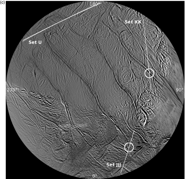
Figure 3. (a) Polar stereographic basemap of Enceladus' south polar terrain (SPT) on which has been plotted all 100 jets sourced in this work. The circles are the 2σ uncertainties; the associated numbers are the jet IDs used in this work. Five sources are indicated by dashed circles because each of these jets appeared in only one observation set; i.e., we are confident of their source locations, but their tilts remain indeterminate. Two crosses indicate two jets, each observed in one image only but each intersected by the shadow of Enceladus, allowing a determination of the fracture they lie on. (b) A 3D map of all 98 jets found in this work whose tilts have been determined. While some jets are strongly tilted, it is clear the jets on average lie in four distinct "planes" that are normal to the surface at their source location. Dotted vectors indicate jets whose sources were determined from images acquired in one observation set only and consequently have a large uncertainty on their tilt. (c) The ISS basemap on which has been plotted the four ground tracks derived from images within sets JJJ, XX, and U. The source locations indicated (Jet #99 in set JJJ) on Baghdad and (Jet #100 on set XX) on Alexandria are the only two determined by direct use of the height of Enceladus' shadow on the jet plus a single ground track. The Set U ground track is discussed in Section 6.(A color version and animation of this figure are available in the online journal.)
Download figure:
Standard image High-resolution image
Figure 4. Top: one image, from set EEE, looking approximately broadside to the fractures and showing a handful of obviously tilted jets. Bottom: the 3D models for the selected jets are projected onto the image. (The bright specks are cosmic ray hits recorded in the ISS detector.)
Download figure:
Standard image High-resolution imageFor each of these independent looks, we wish to determine which portions of the surface were well imaged and how frequently. Consequently, we calculate all across the SPT the minimum height, hmin, that a jet (perpendicular to the surface) needs to reach to be seen by Cassini for each independent look. In this calculation, for each point on Enceladus' SPT, we take into account both the distance from the limb and the curvature of the surface; we also account for the distance from the terminator and, concomitantly, the height of the shadow of Enceladus on the jet. Obviously, for the full vertical extent of a jet to be visible, its source should be located exactly on the limb and this location on the limb should be illuminated by the Sun. However, we can still identify jets even when the bottom portion of them is obscured either by the limb or by the shadow of Enceladus.
In computing the visibility of a selected surface region in a particular viewing geometry, we take as a criterion hmin</= 7 km. Recall that, by early 2012, ∼7 km of the lower portion of the jets residing exactly at the south pole were in darkness. (The majority of our images—86—were taken prior to the start of 2012.) So, with a choice of hmin = 7 km that a region must have in order to be assigned greatest visibility, there is a sizable portion of the SPT whose minimum-sized jets would still be seen in our entire observational sequence according to this criterion. Most jets that are too far over the limb or too far into the dark side of the terminator will escape detection if they fall in a region having hmin>/=7 km, though some very collimated ones might still be detected. The distance from the limb at which a fully illuminated jet that is 7 km tall, seen from equatorial latitudes (as is mostly the case in our data set), would disappear over the horizon is about 58 km.
We take such factors into account in crafting a "visibility" map, Figure 5, which shows, at a glance, the variation in the jet-detection opportunity on the SPT across our observation sequence. Visual inspection of this map shows that the whitest area, the one with the greatest imaging coverage and highest visibility (which corresponds to the number of independent looks being equal to 25, the maximum possible in our data set), is the one closest to the south pole; this results from the near-equatorial sub-spacecraft latitudes from which Cassini images were often acquired. The areas of minimal coverage are on Alexandria Sulcus, with 5–8 independent looks, since often Alexandria Sulcus was too far beyond the limb. The darkest areas have zero visibility.

Figure 5. Map showing the distribution of the visibility of jets across the south polar terrain. The brightest regions have the greatest visibility.
Download figure:
Standard image High-resolution imageThe maximum number of possible independent sightings of any one jet is the same as the maximum number of independent looks, 25; the actual largest number of sightings anywhere on the SPT during the entire 6.5 yr span of our observational sequences is 17, since obscuration of a jet by others makes some observational opportunities fruitless. (Only two jets on Damascus and one jet on a spur of Baghdad have 17 sightings each.) We divide the number of sightings of a jet by the number of independent looks the Cassini ISS had of the surface region containing its source—i.e., the information encoded in our visibility map (Figure 5)—to arrive at a discrete function, Nnorm, giving the normalized number of sightings for all 98 jets; this is our adopted measure of the strength of an individual jet, which is tabulated in Table 2.
(In actuality, the value of hmin = 7 km was chosen a posteriori, as it yields the normalized number of sightings Nnorm = 1, for two jets—one (#21) is on the upper part of Cairo with 6 sightings, and one (#53) is on the spur of Baghdad with 10 sightings—and does not yield any normalized number of sightings greater than 1. (See below.) By coincidence, it also matched the altitude of the shadow of Enceladus on the jets in 2012 March, near the end of our observing sequence.)
3.2. Conversion of Data to Common Format
One of the objectives in this work is to compare the distribution of jetting activity, thermal emission, and tidal stresses across the SPT and search for spatial correlations among them. At the time of writing, Cassini thermal data come in two forms: a low resolution map of CIRS data in which different levels of thermal emission are assigned different colors (Howett et al. 2011), and the much higher resolution "hot spots" detected by (1) VIMS, showing excess 4–5 μm emission very close to Baghdad Sulcus near the south pole (Blackburn et al. 2012), (2) CIRS at high resolution on Baghdad Sulcus (Spencer et al. 2012), and (3) an even higher resolution VIMS detection of one of the hot spots mentioned in (1) (Goguen et al. 2013). At the moment, these high resolution data can be directly compared to our jet source locations and we do so below. However, visually evaluating the correlation between the low-resolution thermal emission and jetting activity is made easier if we present the data from both at the same spatial resolution. This is true of the tidal stresses as well: these can be calculated at every pixel (∼117 meters) along the fractures. However, the horizontal length scale over which the fractures respond to the stresses will be controlled by the brittle layer thickness (a few km), while shorter length-scale variations—conceivably as short as the 0.5 m width of a jet—will arise from variations in local mechanical properties and/or fracture topography, which are not incorporated in our model (below). It is therefore more appropriate to evaluate the similarity of the predicted stresses to the other data, both visually and numerically, if we convert them also to a similar resolution.
For computations of tidal stresses, we use the model described in the supplementary information section of Nimmo et al. (2007). In this model, the instantaneous radial, tangential, and shear stresses due to tides may be calculated at any point within a deforming, spherically symmetric ice shell. Here we assume an ice shell decoupled from the silicate interior by a global ocean. The major simplification that this model makes is its assumption of radially symmetric layers. The extent to which lateral variations in mechanical properties (e.g., Behounkova et al. 2012) will change the answers is currently uncertain, but should be investigated in the future.
Using this simple model, the tidal stresses are resolved onto a particular plane, here assumed to be vertical, representing an individual tiger stripe segment. We calculate the magnitudes of the time-averaged absolute shear stress and the maximum normal stress at each pixel lying along the jet-active portions of each tiger stripe fracture. As we are initially interested in the spatial variations in these stress components and their relation to jet activity and thermal emission, rather than the absolute magnitudes, we have scaled the largest stress values to 1. Time-averaged shear stresses range from ∼20 to 30 kPa and, on individual fault segments, vary by about ±30% around the average value; for simple frictional heating, the local power output should vary by ±70%. Maximum normal stresses range from ∼14 to 85 kPa and on individual fault segments vary up to ±50%; they can be up to three times larger than the shear stresses. (In fact, the current orientation of the tiger stripes with respect to the tidal axis results in near-maximum normal stresses (Nimmo et al. 2007); apparently Enceladus' SPT has settled on the configuration that maximizes normal stresses.) The raw data from these stress calculations are converted to a color map in the same manner described in the next section and displayed in Figure 6.
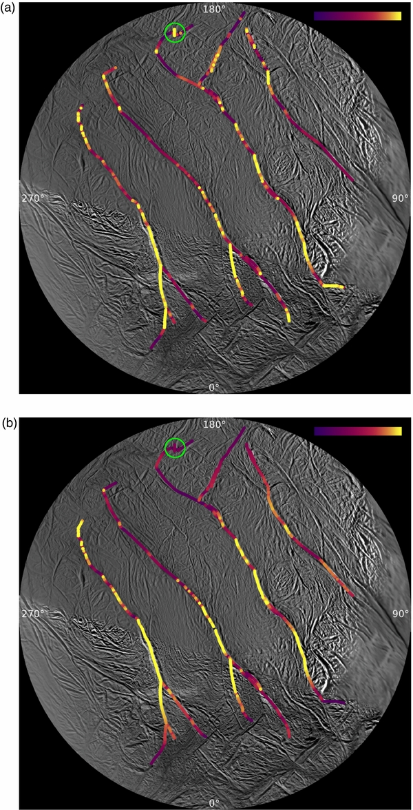
Figure 6. (a) ISS basemap of the SPT on which has been plotted the color-coded relative magnitudes of predicted time-averaged shear stresses. Yellow is the largest, and purple is the smallest. An isolated region of high shear stress is circled. (b) ISS basemap of the SPT on which has been plotted the color-coded relative magnitudes of predicted maximum normal stresses. Yellow is the largest, and purple is the smallest. See the text.
Download figure:
Standard image High-resolution imageNext, we convert the normalized jet activity, Nnorm, and the two components of tidal stress—time-averaged shear stress and maximum normal stress—to the same resolution and ultimately to color-coded maps, similar to the CIRS map, in which the colors have a consistent meaning across all maps.
To begin, we convert the discrete function describing the variation in the normalized number of jet sightings along the fractures, Nnorm, to a smooth, low resolution map by convolving it with a 40 × 40 pixel, or ∼5 × 5 km box. In all cases, we manually adjusted the measured coordinates {lat, lon} of the jet sources to fall exactly on the fractures by locating the point on the fracture nearest the source; that point becomes the adjusted source location, used in performing the convolution. We refer to this convolved quantity as Jet Activity. At this point, we have a smoothed, low resolution 2D array of numbers representing jetting activity and position along each fracture.
In the same manner, we convolve the raw stress calculations shown in Figure 6 with a 5 km square box to produce two smoothed, low resolution 2D arrays representing the two components of stress—shear and normal—versus position along each fracture. We scale the highest values of shear stress and normal stress to 1 and compute frequency histograms of the values contained in these smoothed arrays of scaled time-averaged shear stress, scaled maximum normal stress, and jet activity (already normalized) values; these are shown in Figure 7. Cumulative distributions of these values (i.e., the percentage of the total number of surface points plotted in the histograms that fall below a certain value of activity or stress) are also presented in Figure 7. It is these cumulative distributions to which we assign consistent color mapping.
We assign the color index = 255 (yellow) to the top 15% in all three histograms, and assign the remaining color indices linearly from the 85th percentile downward. The only modification we make is an accommodation of the very likely possibility that there may well be low levels of jetting activity that the ISS cameras cannot image, either because the jets are too short and/or feeble, or because the activity does not take the form of a discrete jet and therefore our procedures do not identify and catalog it. Put another way: shear and normal stresses have been computed along every linear segment of the fractures on the SPT, but discrete jets are not observed everywhere, despite the fact that diffuse activity may be present. To account for this, we assume that scaled shear values </=0.71 and scaled maximum normal stress values </=0.54 in Figure 7 have no counterparts in the histogram of observed jet activity and we thus do not include them in the cumulative distributions (Figure 7). The rough similarities in the shapes of the lower ends of all three cumulative histograms when we exclude the lowest stress values both motivated, and also appear to be consistent with, this approach. The resulting color mapping is shown at the top of each histogram in Figure 7. Using these color assignments, we produce maps of observed jet activity and predicted mean shear stress and maximum normal stress. These, as well as the CIRS map, are shown in Figure 8.
4. CORRELATIONS AMONG SPT PHENOMENA
Visual inspection of these maps immediately reveals their striking similarities. Referring to the Saturn-opposing (lon = 180°) and Saturn-facing (lon = 0°) ends of the fractures as being "upper" and "lower" in the figures, and keeping in mind that the statistics of small numbers will most affect the areas where we had the least number of independent looks—both ends of all the fractures and especially Alexandria Sulcus—we readily see that where ISS finds the greatest jet activity (excepting Alexandria which has the poorest statistics), CIRS finds the greatest thermal emission. Even the relative strengths between the two data sets match nicely: the lower two-thirds of the main trunk of Damascus is hottest (Howett et al. 2011) and also sees the greatest concentration of jetting; the next warmest is the lower part of Baghdad, where we have decreased but still strong jet activity; next, the correspondence is reasonably good in the lowest part of Cairo, and the portion sitting exactly where the upper end of Cairo splits; and finally, to a lesser degree, there is a jetting/thermal emission correspondence in the upper one-third of Alexandria.
From these comparisons we conclude that across the SPT, on large spatial scales, jet activity and thermal emission are well correlated, though which one is producing the other is not evident at this point.
Comparing now the jet activity with the stress maps, we note the following.
- 1.The upper end of Damascus and the lower half of its main trunk (excluding the split-end portion) are sites of both high stresses—shear and normal—and high jet activity.
- 2.The same observations can be made of Baghdad Sulcus, though in neither map are the active regions as spatially extensive on Baghdad as on Damascus.
- 3.Excluding the upper split end of Cairo and its lowest "bend," the three main areas of jetting—upper, middle, and lower—on the remainder of the fracture are also generally regions of greatest stresses of both kinds.
- 4.Only on Alexandria, the fracture that is likely to be most beset by poor statistics, is the correlation between normal stress and jet activity rather poor, though shear and jetting are better matched in the upper part of the fracture.
To assess the statistical significance of these similarities, we compute the linear correlation coefficient between both data sets. That is, we move pixel by pixel along the fractures and at those positions where we have values for all three variables, we read the values from the corresponding maps. From the resulting 1:1:1 arrays of jet activity, shear stress, and normal stress, a standard calculation of the linear correlation coefficient between each pair is computed, giving the degree of correspondence between the two. The coefficient between jetting and shearing is 0.268; the statistical noise in this sample is σ = 0.016. The linear correlation coefficient between jetting and maximum normal stress is 0.267 ± 0.015. To within the uncertainties, these coefficients are identical, and though not large, are positive and statistically significant. This should not be surprising: the correlation coefficient between each of the stress maps on the jet-active segments is 0.70. It is clear that heating and jetting are well correlated across the SPT and concomitantly (Figure 8) all four phenomena exhibit significant correlations among themselves. These results tell us that, though jetting and excess thermal radiation are clearly related, we cannot, on the basis of these comparisons, distinguish which stress component is dominant in its relation to either jet activity or heat emission.

Figure 7. Frequency histograms of the (a) scaled jet activity, (b) scaled time-averaged shear-stress, and (c) scaled maximum normal stress, and their respective cumulative histograms; i.e., the percentage of the total number of surface points that fall below a particular value of (d) jet activity, (e) shear stress, and (f) normal stress. The color-mapping scheme, determined from examination of the cumulative histograms and shown at the top of each histogram, was determined by assigning the top 15% of the distribution to yellow, and linearly scaling the "lower" colors to the lower stress or activity values, taking the lowest value to be either 0 in the jet activity distribution, or the indicated cutoff value in the stress histograms. These color assignments were used in our resulting maps.
Download figure:
Standard image High-resolution imageExamination of the higher resolution VIMS results are far more telling. The IAU system coordinates of two of the three hot spots seen by VIMS during the E11 2010 August 13 close flyby of Enceladus were originally reported in Figure 1 of Blackburn et al. (2012); more carefully measured coordinates of all three hot spots made in the original VIMS data, along with their estimated uncertainties, were supplied by J. Gogeun (2013, private communication). When these coordinates are shifted into the Voyager coordinate system used in this paper, and plotted on our jet source map (Figure 9(a)), we note that they come very close to four source locations (Table 2): #33 (yellow), #34 and #35 (green and cyan, respectively), and #36 (deep blue). (To within their 2σ uncertainties, two of our sources, #34 and #35, with very different tilt directions fall on top of one another and form the middle "composite source location" of this trio.) However, a slight shift of {−20, 12} pixels on the map, equivalent to ∼2.8 km, places the hot spots exactly on the fracture, yields an excellent match between the spatial arrangement of the observed hot spots and that of our jet sources, and leaves the cold spot off the fracture where we have no jets (Figure 9(b)). A shift of this magnitude is well within the estimated VIMS uncertainties of ∼4 km, which includes instrument resolution plus navigation. Contributing uncertainties from the underlying ISS base map can be as high as ∼5 pixels or ∼0.6 km.
An even higher resolution VIMS detection of the hot spot with the lowest southern latitude of the three above occurred during the much closer E18 2012 April 14 flyby (Goguen et al. 2013). This single spot detection, when translated into the Voyager system, also falls within all uncertainties onto jet #33 (Figure 9(a)); a shift of {−13, −3} pixels, equivalent to 1.6 km and equal to the sum of the VIMS error of ±1 km and the error in the underlying map, ∼0.6 km, places it well within the 2σ uncertainty circle of Jet #33 (Figure 9(b)).
Thus, we regard as robust these spatial coincidences between jet sources and hot spots, and we conclude that each of these VIMS hot spots is the thermal footprint of an individual jet (or two) seen in ISS images. Modeling of the spectrum of the thermal emission arising from the VIMS detection of jet #33 revealed the horizontal scale to be ∼9 m and the temperature to be 197 K ± 20 K (Goguen et al. 2013). The significance of these results is discussed in Section 6.
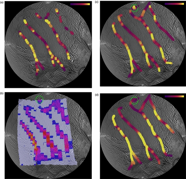
Figure 8. (a) ISS basemap of the SPT on which has been plotted the observed normalized jet activity, calculated and color-coded as described in the text. (b) A CIRS low-resolution map created from thermal emission data collected in 2008 and 2010 (Figure 3 of Howett et al. 2011), laid on the ISS basemap used in this work. From coldest to hottest, the color mapping is pale blue, deep blue, magenta, red, and dark yellow. Note the isolated hot spot at the top of Cairo Sulcus, which is coincident with a location of maximum shear stress, and through which passes a single jet groundtrack. (See the text and Figures 1(f) and 3(b).) (c) The map in Figure 6(a), showing the distribution of time-averaged shear stresses, smoothed with a 40 pixel (or ∼5 km) square sliding box. The same color scheme is used. (d) The map in Figure 6(b), showing the distribution of maximum normal stresses, smoothed with a 40 pixel (or ∼5 km) square sliding box. The same color scheme is used.
Download figure:
Standard image High-resolution image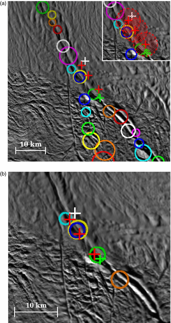
Figure 9. (a) Three VIMS hot spots and one cold "calibration" spot from the E11 Enceladus flyby (Blackburn et al. 2012), and another VIMS hot spot detected during the E18 flyby (Goguen et al. 2013), overlaid as crosses on a magnified portion of Baghdad Sulcus (Figure 3(a)). Translated into the Voyager system coordinates, the {lat, lon} coordinates in degrees are: for E11—lower {−83.00, 26.00}, middle {−84.30, 23.70}, upper {−85.20, 21.50}, and cold spot {−85.75, 24.98}; for E18—{−82.36, 24.74}. The inset shows the absolute 1σ uncertainties in the locations of the E11 VIMS sources (∼4 km) and those of the E18 spot (∼1.0 km). (Note that the coordinates of the E11 hot spots (shown in red) have been kindly re-computed from the original VIMS data by J. Goguen (2013, private communication); the coordinates of the cold spot (shown in white) are taken from Blackburn et al. 2012.) (b) Same as (a), except the VIMS E11 spots have been shifted in unison by {−20, 12} pixels, corresponding to ∼2.8 km, to coincide exactly with the jets' locations on the fracture; the E18 spot has been shifted by {−13, −3} pixels, or ∼1.6 km, also to coincide with the jet's position. These shifts are comparable to the 1σ uncertainties assigned to the VIMS measurements plus the positional errors in the underlying map of ∼0.6 km. To within all uncertainties, the lowest latitude E11 spot and the E18 spot are one and the same and coincide with (green) Jet #33.
Download figure:
Standard image High-resolution image5. TEMPORAL VARIABILITY
One outstanding and obvious question, noted by Hurford et al. (2007), is whether the geysers cycle on and off in synchronicity with the tidal stresses: i.e., does the opening and closing of fractures on a daily schedule turn eruptions on and off? Of course, nature is complex and jets may not completely turn off but merely diminish in vigor during a compressive cycle. Also, other effects can alter the phase of the eruption state from the simple model. Librations in the orientation of Enceladus could change the phase of this cycle and, depending on the type of libration, its periodicity. Possible candidates are physical (1:1) librations, and longer-period librations forced either by Dione or resulting from a secondary spin/orbit resonance; 1:3 (Wisdom 2004) and 1:4 (Porco et al. 2006) have been suggested as the most plausible candidates, although neither is supported by the Iess et al. (2014) gravity measurements.
If individual jets are periodic in their eruptions in accord with this model, it would provide dramatic additional support for the suggestion that normal tidal stresses control the jetting phenomenon, and any difference in phase from that expected from pure tidal forcing might constitute evidence of a libration, which could in turn yield insights into the moon's rotation state and interior structure (Rambaux et al. 2010). Current published upper limits on any librations are 15 (Porco et al. 2006), though this number will certainly be refined in the future. Alternatively, the phase of the eruption might be altered by a delayed response of the ice shell to the tidal forcing, or a delay in the eruption itself. In the first case, the observations may yield insights into the viscoelastic properties of the ice; in the second, into the hydrodynamics of the eruptions and the plumbing of cracks in the ice shell.
A periodicity in the brightness of the plume of material erupting from the south pole was detected in near-infrared data collected by the VIMS instrument (Hedman et al. 2013), lending strong support to the basic tidal control hypothesis, though no attempts were made to model the VIMS data. In Paper 2, we report the discovery of a similar diurnal variation in the spatially integrated brightness of the plume as observed in ISS images, and present our attempts to explain both ISS and VIMS observations in terms of the collection of models mentioned above. At this point, neither the models nor any data set—either the ISS or VIMS plume observations or measurements of Enceladus' surface features made on high resolution Cassini images—are sufficiently precise to distinguish among the various tidal-variation models. Nonetheless, tidal control of the modulation of plume mass production is obvious.
The survey of individual jets we have conducted in this work, where we have multiple observations of the same jet taken at various times and different Enceladus orbital positions, allows us to investigate the temporal variability of individual jets and compare them to the same models used in the integrated study reported in Paper 2. We have in fact found in the present work that 34 jets are demonstrably time-variable and not observed at times and geometrical circumstances when they should have been easily seen: i.e., they are neither obstructed by other jets, too far over the limb, nor in the dark. Of course, even jets observed in their "on" state can be compared to model predictions: finding jets "on" when the model predicts "off" is as informative as the converse.
Since tidal stresses were computed in Paper 2 for the loci of points along the jet-active fractures, and since all jets are located, to within the measurement uncertainties, on either the trunks or split end of the four main fractures, we take as the actual location of an individual jet its adjusted location computer earlier: i.e., that point on the fracture that is nearest the measured location of the jet and consistent with its measured uncertainties. This ensures that the location of the computed stress is the same as the (adjusted) location of the jet.
Paper 2 investigates three classes of models describing plume activity: one in which normal stresses due to eccentricity tides plus a time delay are responsible; a second in which normal stresses due to eccentricity tides plus a 1:1 in-phase libration control the activity; and a third in which activity occurs when tidal stresses are right lateral. For each of the 3 models investigated in Paper 2, we computed the magnitude and phase of the relevant stresses at the adjusted locations of each of the 98 jets at the time it was, or was unambiguously not, observed. (For illustrative purposes, we show in Figure 10, for one jet, #73, how the normal stress at the adjusted jet location should vary over an Enceladus orbit for one model, and compare those results to the observed states of the jets.)

Figure 10. Plot of the variation in normal tidal stresses, expected for the model that includes eccentricity tides plus a 1:1 physical libration of 07 amplitude (Paper 2), at the adjusted location of Jet #73. Positive stresses are extensional, negative, compressional. The black dots mark those observations where either the eruption state was ambiguous or the jet, even if on, would not have been clearly visible, for example, it was beyond the terminator, obscured by other jets, over the limb, etc.
Download figure:
Standard image High-resolution imageThen, for each jet, we culled from the entire set of observations the ones of which we were most confident that the jet was clearly present or clearly not present when it should have been: i.e., it was not out of the field of view, obscured by other jets, beyond the limb, beyond the terminator, or difficult to see because of Enceladus' shadow or low resolution. From this reduced set, we produced histograms binning the frequency of jet observations of a particular eruptive state, either on or off, across the spectrum of tidal stresses, normalized to vary from −1 to 1: positive values are tensile (open fractures) or right-lateral, and negative compressive (narrow or closed) or left-lateral. We produced such histograms for each of the three tidal stress models used in Paper 2. These histograms are shown in Figure 11. If the eruption states of the entire collection of jets were, on average, being controlled by the tidal stresses as predicted by Hurford et al. (2007), we should find a greater correlation of "on" with positive stresses and "off" with negative. To test this expectation, we also computed the statistic

Figure 11. Histograms showing the number of jets unambiguously observed in both "on" (above) and "off" (below) eruption states that occupy particular (scaled) stress intervals for each of the three models examined in Paper 2: (a) time delay, (b) 1:1 physical libration, and (c) right-stepping shear motion. The statistical quantity γ for each model measures the likelihood of an orbital correlation. Values close to unity indicate no statistical correlation.
Download figure:
Standard image High-resolution imageThe numerator of this quantity evaluates whether jets are seen more frequently when they are predicted to be active; the denominator normalizes this quantity appropriately, by correcting for the fact that positive stress cases may be seen more frequently than negative stress cases (or vice versa). For all three models, we find γ ∼ 1. It is clear from this that for no model is there on average a correlation between the eruption state of individual jets and the expected phase of the local normal stress. That is, despite the clear variation in the brightness, hence mass, of the integrated plume with orbital phase that both ISS and VIMS see (Hedman et al. 2013; Paper 2), we find that the on and off states of individual jets are not related, on average, to local tidal stress in the same manner. We discuss this result below.
6. DISCUSSION
The obvious spatial correspondences, at low resolution, of thermal emission, jet activity, and tidal stresses along the jet active segments of the tiger stripe fractures, and the correspondences at high resolution between individual jets and hot spots, have important implications for the generation and transport of the heat observed radiating to space, the source of the material producing the jets, the mechanisms driving these two phenomena, and the current state and thermal history of Enceladus.
Earlier work (Nimmo et al. 2007) suggested that shear stresses were likely responsible for producing the (bulk of the) observed heat and vapor. Ice shell models predict surface fractures that extend to rather shallow depths, just a few kilometers, into the shell's brittle layer. If the jet-active fractures we see at the surface are shallow and do not connect to the sea below, then the water and vapor in the jets must arise from melting and vaporization of the crack walls due to heating in the brittle layer. This could in theory explain the association of jetting and thermal emission with the locales of the greatest shear stresses.
However, this interpretation has several problems. First, it would not explain the salinity of the near-surface jet particles which would be expected if the icy particles are frozen droplets of salty water deriving from a sea in contact with the rocky core of the moon (Postberg et al. 2011).
Second, shear stresses will be greatest at the base of the brittle layer where the pressure is largest, and will produce a surface hot spot with a horizontal spatial scale comparable to its thickness: i.e., a few kilometers. This is inconsistent with the observed sizes of the small-scale hot spots detected by VIMS and which are shown in this work to be the thermal signature of individual geysers. In contrast, the size of a thermal spot produced by deposition of latent heat in the near-surface region of a narrow, <1 m conduit delivering vapor from below will be a few tens of meters (Nakajima & Ingersoll 2012; M. Nakajima 2014, private communication), consistent with the observations. Third, the CIRS spectral data (Abramov & Spencer 2009) are inconsistent with conduction from a laterally distributed subsurface source of the kind shear heating would produce, and instead argue for small fractions of the surface being heated to high temperature.
Finally, while jet activity and thermal emission are correlated with shear stresses, they are also correlated with normal stresses, making it unclear that shear stresses are the driving mechanism. Our interpretation that normal stresses are playing the starring role is consistent with the observations of time-variable plume strength found in both VIMS (Hedman et al. 2013) and ISS (Paper 2) data. Moreover, the shear-heating model implies a rate of tidal heating that is constant over the diurnal tidal cycle, an interpretation that is inconsistent with the observations.
A more plausible explanation is that the associations we find exist because water-filled cracks can propagate upwards from the base of the ice shell through the already weakened ice of a deep tiger stripe fracture zone and extend through tens of kilometers of ductile ice (Figure 12). This system would provide ready pathways for liquid and vapor and the latent heat they carry to reach the surface and produce what is observed.

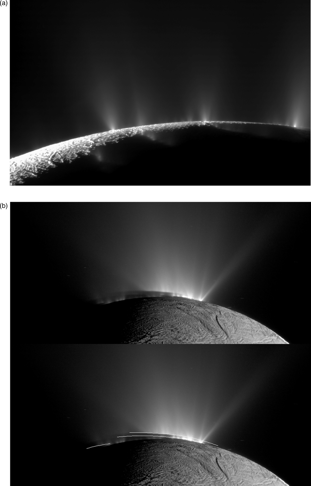
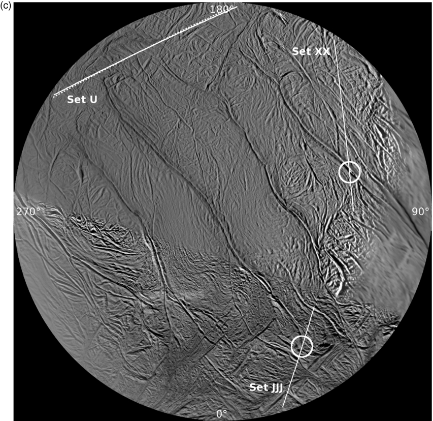
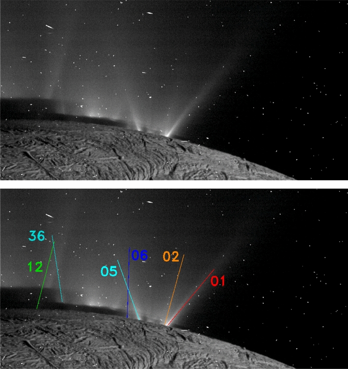
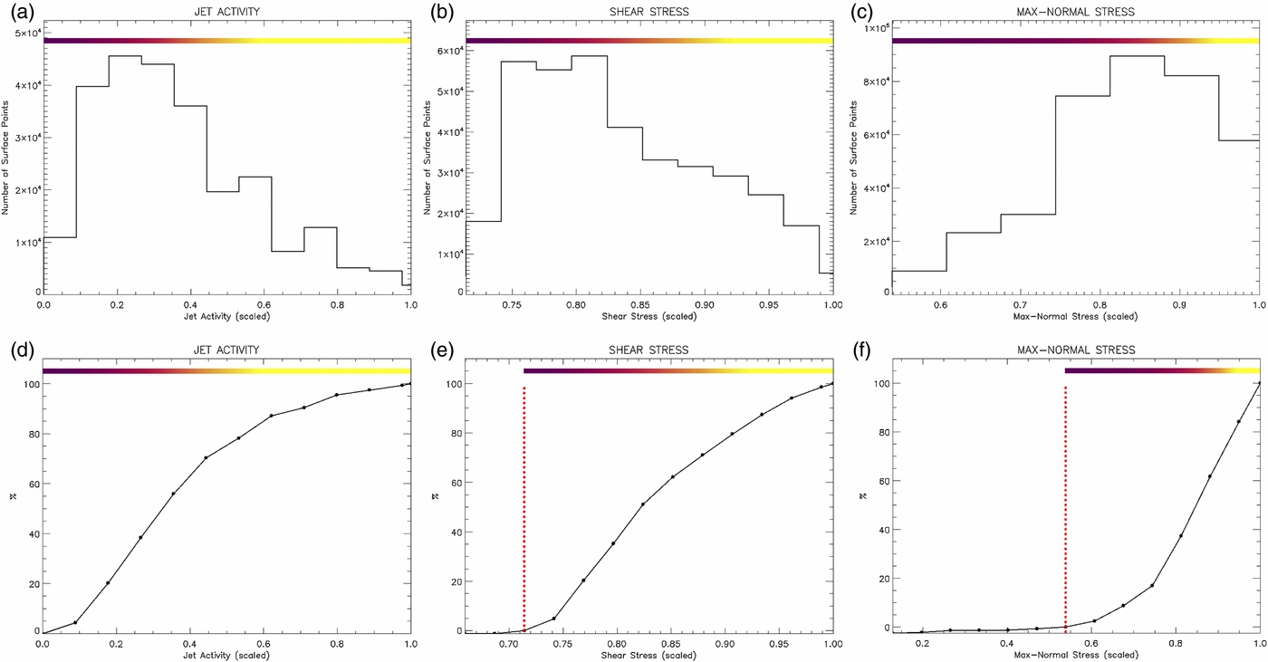
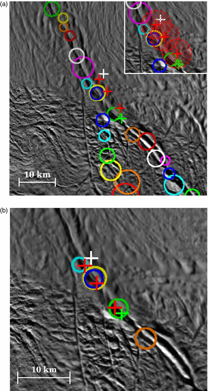
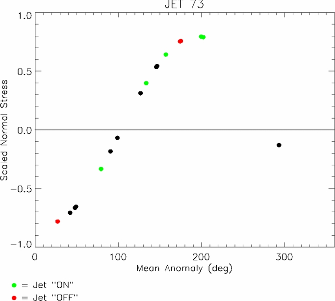
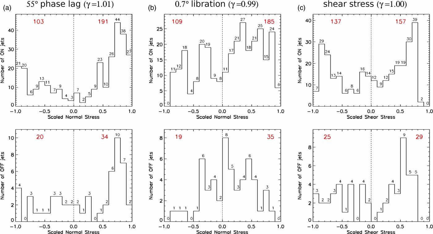
Figure 12. Schematic illustrating current knowledge of the (a) global, (b) regional, and (c) small-scale physical and thermal structure and processes relevant to Enceladus' geysering activity, within and at the surface of the moon, inclusive of the results presented in this work. In the south polar region, the sea is ∼10 km thick; the ice shell above it is ∼30–40 km thick (Iess et al. 2014), comparable to the separation between the main fractures. Narrow cracks extend upwards from the sub-surface sea all the way to the surface, through both ductile and brittle layers of the ice shell. Liquid water under pressure fills the cracks, keeping them open even throughout the ductile layer and providing a conduit for vapor and sea water to reach the near-surface. Other processes, such as exsolution of volatiles, can drive vapor and water droplets all the way to the surface, forming geysers and condensing close to the surface, depositing latent heat. This heat is observed by Cassini's long-wavelength infrared instruments as the anomalous thermal radiation from the jet-active regions of the fractures. The subsurface regions immediately surrounding the sea and the cracks bearing water and vapor are expected to be warm. Regional heating from tidal flexing is also expected to be present, but is so far undetected. The ice shell beneath the SPT is likely the only place on the moon today where convection is occurring.
Download figure:
Standard image High-resolution image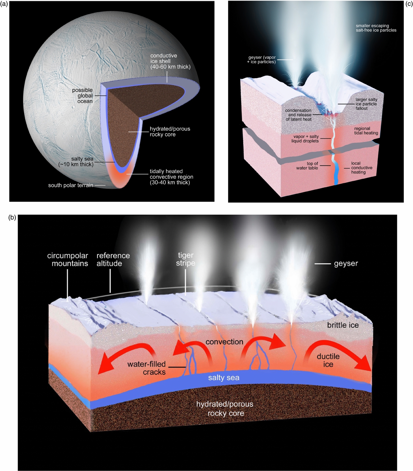
In this scenario, narrow cracks must extend through the ice shell all the way down to the sea. The thickness of the ice shell at the south pole above the liquid layer has been estimated to be ∼30–40 km (Iess et al. 2014). Crack propagation through the brittle layer only a few kilometer thick is easy; not so for the ductile layer, which first must be opened—i.e., the crack must be initiated—and then kept open by some mechanism.
Crawford & Stevenson (1988) point out that despite the expectation that warm ice would have to be strained faster than the diurnal cycle time of the tidal stresses in order to crack, warm ice may be weaker than cold ice (Parameswaran & Jones 1975) and if the stress is applied continuously and periodically, stress-corrosion cracking can initiate a narrow fracture. In fact, water-filled fractures are known to exist at the base of terrestrial ice sheets (e.g., Jezek & Bentley 1983), despite the warm temperatures of the ice there; in some cases, these fractures develop because of ocean tidal flexing (e.g., Vaughan 1995).
Once initiated, water-filled cracks can propagate upwards through a ductile layer. For this to occur, two conditions—mechanical and thermal—must be satisfied. The mechanical condition requires that the stresses driving crack propagation are sufficient to overcome the fracture toughness of ice; the thermal condition requires that the water in the crack not freeze significantly during propagation.
Following the approach of Crawford & Stevenson (1988), it can be shown that there exists a minimum tensile stress σmin for crack propagation to occur based on a balance between the work required to overcome fracture toughness and the work available through the tidal stresses. It is given by

where K is the fracture toughness of ice, g is gravity, and Δρ is the ice–water density contrast. Taking g = 0.11 ms−2, Δρ = 80 kg m−3, and K = 105 Pa m1/2 (Van der Veen 1998), we find that the minimum tensile stress is 5 kPa. Since tidal stresses on Enceladus are likely ∼100 kPa (e.g., Nimmo et al. 2007), there is no problem in propagating cracks. The maximum crack length lmax is given by
where σ is the stress. For Enceladus, crack lengths of ∼20 km—within a factor of two of Enceladus' ice shell thickness at the south pole—are expected with tidal stresses of 100 kPa. Cracks propagating through thicker shells, as has Enceladus, are possible if additional sources of tensile stress, such as ice shell freezing and thickening (Manga & Wang 2007) or thermoelastic stresses, are present.
The combined thermal-mechanical problem is addressed by Alley et al. (2005) and (for silicates) by Rubin (1995). Two timescales are important: the crack propagation timescale (tp)—which is limited by the ability of turbulent water to flow up the crack—and the freezing timescale (tf). The ratio of these two quantities determines whether a crack will propagate before freezing or not. From Crawford & Stevenson (1988) we can write:
where w is the crack width, l the length, and ρ the water density. For Enceladus parameters, the propagation velocity is a few cm s−1 for w = 0.1 m and ∼0.1 m s−1 for w = 1 m. The freezing timescale is tf ∼ w2/κ, where κ is the thermal diffusivity. We can therefore calculate a critical crack width wcrit for propagation to occur

Taking κ = 10−6 m2 s−1, we find that cracks wider than half a meter or so will propagate through the bulk of Enceladus' ice shell before freezing. An alternative to Equation (4) incorporating viscosity (Schubert et al. 2001, Equation (4.5.46)) results in a velocity roughly one order of magnitude faster, so our minimum crack width estimate is conservative.
If such cracks exist, they must be filled with liquid water. If the liquid column is connected to a subsurface sea at the bottom, its upper surface will adjust to a height that is ∼92% (the ratio of the densities of ice to pure liquid water) of the distance between the sea and the surface (Crawford & Stevenson 1988), or ∼3 km from the surface for a 30 km thick ice shell. This value will change somewhat depending on the heat flux, thermal conductivity of the ice, friction between the fluid and the crack walls, the composition of the ice shell (pure ice or a dense clathrate), etc. But whatever the equilibrium level of the liquid, it could, from there, get all the way to the surface with assistance from a suite of possible processes: the rapid exsolution of gases (Crawford & Stevenson 1988; Matson et al. 2012), pressure due to topographic variations (Showman et al. 2004), or pressurization of the underlying sea due to freezing and ice-shell thickening (Manga & Wang 2007). Also, if any cracks propagating from above in the brittle layer join a crack coming from below, the immediate exposure to vacuum will presumably cause violent release (Matson et al. 2012).
The solids in this scenario are the salty water droplets entrained in the pinched-off bubble of vapor that rises from the top of the water column in the cracks (Crawford & Stevenson 1988); i.e., maybe from a depth of only a few kilometers. Once the upward traveling water droplets encounter vacuum, they freeze and are observed as jets by ISS. One consequence of this scenario is that liquid water may exist within a few kilometers of the surface or even, in limited amounts, reach the surface.
Germane to this discussion is the prediction that jets will turn on and off in synchronicity with the opening and closing of fractures under normal tidal stresses (Hurford et al. 2007). While we have demonstrated here that such behavior is not observed on a jet-by-jet basis, there is solid evidence that the entire plume of material escaping the SPT does vary in phase with the orbital position of Enceladus (Hedman et al. 2013; Paper 2). There may be no inconsistency here. In Paper 2, we present evidence that the strength of the plume, and presumably the average strength of individual geysers, is modulated by varying tidal stresses over the course of an orbit but never fully goes to zero: i.e., the jet-active regions of the fractures, on average, never fully close but only narrow during the compressive phase of the cycle. The geysers eventually fail and turn off not on a daily timescale but when an individual vent becomes clogged with ice from condensed vapor, probably on a much longer timescale (Porco et al. 2006; Ingersoll & Pankine 2010).
Of course, it is not implausible that there are local variations and in some locales, within the brittle layer, shearing is the dominant effect at least for a time. One such locale may be at the upper end of Cairo where we find a region of high shear but not of high normal stress (Figure 6) coincident with a large-scale, isolated "hot spot" seen in the CIRS map (Figure 8(b)). It is a location where the "hook" of Cairo is crossed by a short but prominent fracture of high mean shear stress; it is also a site that is crossed by one of our source-less ground tracks from the sighting of a jet in only one set of images (Figure 3(b)). If shearing, and not tension, is responsible for the thermal emission there, we would expect the size of the hot spot to be kilometers in size. Perhaps Cassini's last flybys of Enceladus at the end of 2015 will be able to address this. Of course, such a geyser is likely not long lived, as abundant liquid water production will reduce the friction coefficient and cause shear heating eventually to cease.
It appears from this work that normal stresses are playing the dominant role in the activity, including the emitted heat, observed across the SPT of Enceladus, and that shear heating is of at most minor importance. And while this work lends support to the notion that heat and material stored below in a regional sub-ice-shell sea are transported to the surface via conduits that rise to the surface in the tiger stripe fractures, what is not yet clear is whether any of the water erupting from below and its latent heat are being produced today. If so, regional tidal heating (as opposed to localized shear heating) must be taking place today, and Enceladus' eccentricity is currently decreasing because the equilibrium heating rate is exceeded (Meyer and Wisdom 2007). CIRS may be able to detect this regional heating later in the Cassini mission, during southern winter: uncertainties in the thermophysical properties and albedo of the SPT mean that a background regional heat flow of at least several GW could be present but indistinguishable from solar heating (Howett et al. 2011).
Alternatively, Enceladus' eccentricity and heat production could be in steady state, in which case it is heat produced at an earlier epoch that is currently being mined. In this case, the regional sea will be shrinking due to direct mass loss at ∼200 kg s−1 and perhaps also progressively freezing (Roberts & Nimmo 2008; Behounkova et al. 2012). Geyser activity and mass loss, however, may be self-limiting as the result will be subsidence of the ice shell, resulting in compression and prolonged closure of the fractures.
Why are the tiger stripe fractures the sites of jetting and thermal emission and not other fractures on the SPT? Though the SPT is highly fractured on various spatial scales, the stripes are clearly the most prominent: they are the longest continuous fractures, with the greatest surface relief and the largest widths. They also have the widest separations: from fracture to fracture, about 35 km (Porco et al. 2006). If they are in fact tension cracks, perhaps produced in an earlier epoch of much larger eccentricity and tidal stresses, as in the model of Behounkova et al. (2012), their 35 km spacing should reflect the depth to which they have propagated and hence, very likely, the thickness of the ice shell during that epoch. It is notable, and consistent with the tensile crack hypothesis, that the thickness of the SPT ice shell, deduced from Cassini's gravity results, is 30–40 km (Iess et al. 2014), and that the tiger stripe fractures are oriented perpendicular to the direction of the largest tensile stress (Nimmo et al. 2007). Today these fractures would be the vertical zones of greatest weakness carved through the ice shell, and the planes in which today's maximum normal stresses would first open narrow cracks to be filled with water under pressure.
However, it is important to note that the majority of the vapor observed by the Cassini UVIS as well as particles coming from Enceladus observed by the CDA, point to a source of material broadly distributed across the SPT (Hansen et al. 2011; Postberg et al 2011). Could finer fractures across the SPT be deep enough to reach a subsurface sea? Or are the widely distributed particles and vapor arising instead from evaporation from the warm surfaces of shallow cracks across a tidally heated SPT, with some of the vapor undergoing adiabatic expansion and condensation into solids? Or could there be lower speed eruptions along broad regions of the tiger stripe fractures so that sheets of material instead of collimated jets are formed? In this last case, the gas and entrained particles would emerge from the fractures with a (relatively) more rapid lateral expansion, forming a diffuse, broadly distributed cloud. The answer is not presently clear and may need to await both a detailed comparison among CDA, UVIS, and ISS results, and a final determination of the level of regional thermal emission, if any, during Cassini's last flybys near the end of 2015.
We note finally that maximum geysering activity, as well as maximum stresses, are not uniformly distributed over the SPT but instead are concentrated in the Saturn-facing hemisphere (Figure 8). The analyses of two stellar occultations and one solar occultation by the vapor plume above the SPT observed by UVIS all give consistent fluxes of 200 kg s−1 if an elongate shape, offset from the pole into the Saturn-facing hemisphere, is assumed (Hansen et al. 2011). This is consistent with the spatial distribution of jetting across the SPT and all these observations agree with the predicted orientation of the stress patterns as well: the tiger stripes in the Saturn-facing hemisphere are on average more nearly aligned with the tidal axis direction. Why the tiger stripes should have this particular configuration is unclear, but may be related to the evolution of tidal deformation experienced by Enceladus across time.
7. CONCLUSIONS
In a survey conducted with the Cassini Imaging Science Subsystem experiment (ISS), ∼100 distinct, narrow geysers have been identified and found to erupt from either the main trunks or split ends of the four main "tiger stripe" fractures crossing the south polar terrain (SPT) of Enceladus. Comparison of the results presented here with the results of other Cassini instruments, e.g., UVIS and CDA, indicates that the material erupting in the form of distinct jets is only part of the total amount of material (solids and vapor) leaving the SPT. Nonetheless, the greatest jetting activity is clearly correlated with those locales along the fractures exhibiting greatest thermal emission; it is also correlated with the regions along the fractures undergoing the greatest tidal stresses.
Individual jets along Baghdad Sulcus near the south pole have been found from this work to be spatially coincident, to within all considered uncertainties, with several small-scale (tens of meters) hot spots detected by the VIMS instrument. We conclude from this that the hot spots are the thermal signature of the geysering process. The small size of these hot regions, with temperatures near 200K, rules out shear heating in the brittle layer as the origin of the jets and heat; instead, their size is consistent with the thermal signature expected from near-surface condensation of vapor (and liquid) erupting through narrow conduits and the subsequent release of latent heat.
Normal (tensile) stresses are the main mechanism "driving" the south polar activity by opening narrow vertical pathways within the tiger stripe fractures zones that reach a body of liquid below, thereby allowing the delivery of water vapor and liquid, and the latent heat they carry, to reach the surface, forming the geysers and depositing near-surface latent heat. Theoretical considerations of the propagation and maintenance of water-filled cracks support the notion that these water-delivering pathways can extend through the entire SPT ice shell. Along with the rather large average solid/vapor ratio in the geysers and the salinity of the jet particles, the work presented here points to a deep sea, below the SPT ice shell, as the source of the eruption materials and the observed heat. The top of the liquid water table within the cracks supplying the geysers may lie within a few kilometers of the surface; liquid water in small quantities may in fact reach all the way to the surface. These results have important implications for future studies of, and missions to, Enceladus.
About one-third of the geysers surveyed in this work have been observed to cycle on and off over the 6.5 yr spanned by our data set, but do not do so with phases predicted by the three variants of the basic eccentricity-tide model, examined in depth in Paper 2, that describes the diurnal variation in SPT tidal stresses, even though the spatially integrated plume is clearly tidally modulated. From this we conclude that the strength, or mass production rate, of individual geysers is modulated by the tides, but a different process turns them on and off. It is most likely that the vents supplying the geysers are ultimately choked off by the very process that makes them warm: the near-surface condensation into ice of vapor and liquid.
Our findings have important implications for the present state and thermal history of Enceladus' interior. If, as we have shown, the heat emitted from the tiger stripe fractures is not being produced by shear stresses, then some fraction of the erupting water (vapor and liquid) and its latent heat must have been generated at an earlier time. Whether any of it is the result of melting from present-day regional tidal dissipation remains to be seen.
Bulk viscous heating by tidal flexing of the ice shell underlying the SPT is expected at some level and might be detectable by the CIRS instrument in the form of broadly distributed, regional thermal emission. Opportunities to make such observations of the SPT during the moon's southern winter, when the SPT will be in total darkness and sunlight will not be a contaminating factor, will present themselves during the last few months of 2015, when Cassini will make its final close encounters with Enceladus.
We appreciate the assistance of the members of the CICLOPS group in planning, sequencing, and executing the image sequences used in this work. We thank Thomas Roatsch and the ISS DLR group for the creation of the ISS basemap. We thank Jay Goguen for assistance in the interpretation of VIMS high resolution data, Paul Helfenstein for fruitful conversations about uncertainties, Juergen Schmidt for useful comments about styles of eruptions, and Ron Miller for his patience in the construction of Figure 12. Finally, we thank the referee, Dave Stevenson, for his insights and very helpful suggestions. C.C.P. acknowledges support from NASA CDAP and the Cassini project, and F.N. from the CDAP-PS program.
Footnotes
- 3
The South Polar Terrain (SPT) is identified as the region poleward of ∼55° S latitude that is circumscribed by a continuous chain of mountain ridges and valleys, and crossed by four prominent fractures.
- 4
It is plausible that significant regional heat is also present but its flux is below the detection limit of the CIRS instrument. Consequently, the direct contribution of bulk viscous heating today is at the moment unknown.
- 5
What is first identified may be not a single jet but a row of several jets, one behind the other, along the line of sight. Only with images taken from look angles sufficiently separated from the first image can each jet be eventually identified by triangulation.