


ABSTRACT
We report the discovery of HATS-5b, a transiting hot Saturn orbiting a G-type star, by the HATSouth survey. HATS-5b has a mass of Mp ≈ 0.24 MJ, radius of Rp ≈ 0.91 RJ, and transits its host star with a period of P ≈ 4.7634 days. The radius of HATS-5b is consistent with both theoretical and empirical models. The host star has a V-band magnitude of 12.6, mass of 0.94 M☉, and radius of 0.87 R☉. The relatively high scale height of HATS-5b and the bright, photometrically quiet host star make this planet a favorable target for future transmission spectroscopy follow-up observations. We reexamine the correlations in radius, equilibrium temperature, and metallicity of the close-in gas giants and find hot Jupiter-mass planets to exhibit the strongest dependence between radius and equilibrium temperature. We find no significant dependence in radius and metallicity for the close-in gas giant population.
Export citation and abstract BibTeX RIS
1. INTRODUCTION
Transiting planets are the best characterized planets outside of our solar system. The transit geometry allows us to measure the mass and radius and characterize the atmosphere (e.g., Charbonneau et al. 2002; Deming et al. 2005) and dynamics (e.g., Queloz et al. 2000) of individual planets. As a result of the discoveries from wide-field ground- and space-based photometric surveys (e.g., Bakos et al. 2004, 2013; Pollacco et al. 2006; Borucki et al. 2010), statistical studies have revealed that close-in gas giants are rare (e.g., Howard et al. 2012; Fressin et al. 2013), have relatively dark albedos (e.g., Cowan & Agol 2011), and are found preferentially around metal-rich stars (e.g., Santos et al. 2004; Buchhave et al. 2012).
Previous studies have also explored the effect of irradiation and composition in inflating the radius of gas giants (e.g., Guillot et al. 2006; Enoch et al. 2011; Béky et al. 2011; Enoch et al. 2012). In particular, Enoch et al. (2011, 2012) found that the radii of Saturn-mass planets are more dependent on metallicity than those of Jupiter-mass planets, revealing a mass dependence to the inflation mechanisms.
Intensive ground-based follow-up observations are extremely important for the characterization of transiting gas giants. Due to the mass degeneracy in the gas giant regime, Saturns, Jupiters, and brown dwarfs cannot be distinguished from discovery transit photometry alone. The mass degeneracy is a major limitation against using the Kepler candidate sample to study mass-dependent statistics of close-in gas giant planets. The rarity of close-in gas giants, as well as the relative difficulty of characterizing hot Saturns compared to hot Jupiters, leaves the hot Saturn regime still poorly explored. Of the 299 confirmed transiting planets,14 only 23 have masses in range of Saturn (0.1 < Mp < 0.5 MJ) and are found in close-in orbits (P < 10 days). As a result, our statistical understanding of the hot Saturn population is relatively less mature.
In this study, we report the discovery of the transiting hot Saturn HATS-5b by the HATSouth survey. The HATSouth discovery and photometric and spectroscopic follow-up observations are detailed in Section 2. Analyses of the results, including derivation of host star parameters, global modeling of the data, blend analyses, and constraints on the wavelength-radius relationship, are described in Section 3. In Section 4, we revisit some of the statistical trends for the close-in gas giant population and discuss HATS-5b in the context of the known hot Saturns and hot Jupiters.
2. OBSERVATIONS
2.1. Photometric Detection
The transit signal around HATS-5 was first detected from photometric observations by the HATSouth survey (Bakos et al. 2013). HATSouth is a network of identical, fully robotic telescopes located at three sites spread around the Southern Hemisphere, allowing continuous coverage of the surveyed fields. Altogether 8066 observations of HATS-5 were obtained by the HATSouth units HS-1 in Chile, HS-3 in Namibia, and HS-5 in Australia from 2009 September to 2010 December. Each unit consists of four 0.18 m f/2.8 Takahasi astrographs and Apogee 4K × 4K U16M Alta CCD cameras. Each telescope has a field of view of 4° × 4°, with a pixel scale of 3 7 pixel−1. The observations are performed with 4 minute exposures through the Sloan r' filter.
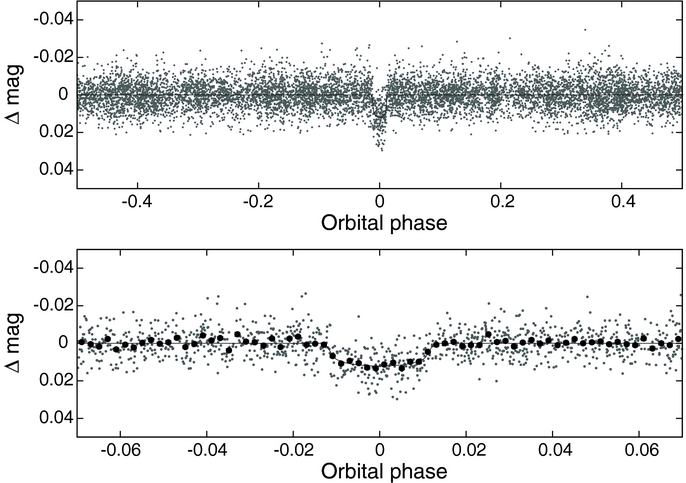
Discussions of the HATSouth photometric reduction and candidate identification process can be found in detail in Bakos et al. (2013) and Penev et al. (2013). Aperture photometry was performed and detrended using External Parameter Decorrelation (EPD; Bakos et al. 2007) and Trend Filtering Algorithm (TFA; Kovács et al. 2005). Transit signals were identified using the Box-fitting Least Squares analysis (Kovács et al. 2002). Table 1 summarizes the photometric observations for HATS-5. The HATSouth discovery light curve is plotted in Figure 1.

Figure 1. HATSouth r'-band discovery light curve, unbinned, and folded with a period of P = 4.7633872 days, as per the analysis in Section 3. Solid line shows the best-fit transit model. The lower panel shows the transit region of the light curve. Dark filled points represent the light curve binned at 0.002 in phase.
Download figure:
Standard image High-resolution imageTable 1. Summary of Photometric Observations
| Facility | Date(s) | Number of Imagesa | Cadence (s)b | Filter |
|---|---|---|---|---|
| HS-1 (Chile) | 2009 Nov–2010 Dec | 3953 | 290 | Sloan r |
| HS-3 (Namibia) | 2009 Sep–2010 Dec | 3241 | 288 | Sloan r |
| HS-5 (Australia) | 2010 Sep–Dec | 900 | 287 | Sloan r |
| ESO/MPG 2.2 m/GROND | 2012 Oct 10 | 178 | 93 | Sloan g |
| ESO/MPG 2.2 m/GROND | 2012 Oct 10 | 107 | 93 | Sloan r |
| ESO/MPG 2.2 m/GROND | 2012 Oct 10 | 214 | 93 | Sloan i |
| ESO/MPG 2.2 m/GROND | 2012 Oct 10 | 211 | 93 | Sloan z |
| ESO/MPG 2.2 m/GROND | 2012 Dec 11 | 159 | 144 | Sloan g |
| ESO/MPG 2.2 m/GROND | 2012 Dec 11 | 160 | 144 | Sloan r |
| ESO/MPG 2.2 m/GROND | 2012 Dec 11 | 162 | 144 | Sloan i |
| ESO/MPG 2.2 m/GROND | 2012 Dec 11 | 162 | 144 | Sloan z |
Notes. aOutlying exposures have been discarded. bMode time difference between points in the light curve. Uniform sampling was not possible due to visibility, weather, and pauses.
Download table as: ASCIITypeset image
2.2. Spectroscopy
Spectroscopic confirmation of HATS-5b consisted of separate reconnaissance observations to exclude most stellar binary false-positive scenarios that can mimic the transit signal of an exoplanet. High-resolution, high signal-to-noise (S/N) measurements of the radial velocity (RV) variation for HATS-5 were then obtained to confirm the planetary status of HATS-5b. The spectroscopic follow-up observations are presented in Table 2.
Table 2. Summary of Spectroscopic Observations
| Telescope/Instrument | Date Range | Number of Observations | Resolution | Observing Mode |
|---|---|---|---|---|
| Reconnaissance | ||||
| ANU 2.3 m/WiFeS | 2012 Aug 4 | 1 | 3000 | RECON Speca |
| ANU 2.3 m/WiFeS | 2012 Aug 4–6 | 3 | 7000 | RECON RVb |
| Euler 1.2 m/Coralie | 2012 Aug 21–2013 Feb 27 | 9 | 60,000 | ThAr/RECON RV |
| ESO/MPG 2.2 m/FEROS | 2012 Nov 21–2013 Feb 27 | 14 | 48,000 | ThAr/RECON RV |
| High resolution radial velocity | ||||
| Subaru 8.2 m/HDS | 2012 Sep 20–22 | 9 | 60,000 | I2/RVc |
| Magellan 6.5 m/PFS | 2012 Dec 28–2013 Mar 4 | 12 | 76,000 | I2/RV |
Notes. aReconnaissance observations used for initial spectral classifications. bReconnaissance observations used to constrain the radial velocity variations. cHigh-precision radial velocities to determine the spectroscopic orbit of the planet.
Download table as: ASCIITypeset image
Low-resolution reconnaissance observations were performed using the Wide Field Spectrograph (WiFeS; Dopita et al. 2007) on the Australian National University (ANU) 2.3 m telescope at Siding Spring Observatory, Australia. A flux-calibrated spectrum was obtained at R ≡ λ/Δλ = 3000 to provide an initial spectral classification of HATS-5 as a G dwarf with Teff = 5300 K, log g = 4.5, and [Fe/H] = 0. These stellar parameters are later refined by higher resolution observations (Section 3). Multi-epoch observations at R = 7000 confirmed that the candidate did not exhibit >1 km s−1 RV variations. Such velocity variations are indicative of eclipsing stellar binaries, which have so far made up  of HATSouth candidates. Details of the WiFeS follow-up procedure and stellar binary identification process can be found in Bayliss et al. (2013) and Zhou et al. (2014). Candidates that pass the WiFeS vetting process are passed on to higher resolution observations.
HATS-5 received nine high-resolution (R = 60, 000) reconnaissance RV observations with the CORALIE spectrograph on the Swiss Leonard Euler 1.2 m telescope at La Silla Observatory, Chile, and 14 R = 48, 000 observations with the FEROS spectrograph on the ESO/Max Planck Gesellschaft (MPG) 2.2 m telescope at La Silla. Detailed descriptions of the acquisition, reduction, and analyses of the CORALIE and FEROS observations can be found in the previous HATSouth discovery papers (Penev et al. 2013; Mohler-Fischer et al. 2013; Jordán et al. 2014). Velocities from these observations allowed us to constrain the RV orbit semi-amplitude to be <45 m s−1.
The upper limit RV constraints from CORALIE, FEROS, and WiFeS indicated that HATS-5b is a low-density gas giant. High-S/N, high-resolution observations were required to determine the RV orbit of the system. Velocities of HATS-5 were obtained by the Planet Finding Spectrograph (PFS) on the 6.5 m Magellan Baade telescope at Las Campanas Observatory, Chile, and the High Dispersion Spectrograph (HDS) on the 8.2 m Subaru telescope at Manua Kea Observatory, Hawaii. The PFS and HDS velocities and bisector spans are presented in Table 3, and the RV orbit is plotted in Figure 2.

Figure 2. Top panel: radial velocities (RVs) phase folded according to the period from the global modeling are shown. Measurements from Magellan/PFS are plotted as dark filled circles, Subaru/HDS as open triangles. The best-fit model is plotted by the solid line. The best-fit absolute velocity offset from each instrument has been subtracted from the observations. An independent Lomb–Scargle analysis of the RV data set was performed, showing that the RV period is consistent with the photometric transits. Middle panel: residuals of the RV measurements from the best-fit model. The error bars have been inflated such that the χ2 per degree of freedom is unity for each instrument. Bottom panel: bisector spans (BSs) are plotted for velocities from Subaru/HDS. Note the different scales for each panel.
Download figure:
Standard image High-resolution imageTable 3. Relative Radial Velocities and Bisector Span Measurements of HATS-5
| BJD | RVa | σRVb | BS | σBS | Phase | Instrument |
|---|---|---|---|---|---|---|
| (2 400 000+) | (m s−1) | (m s−1) | (m s−1) | |||
| 56190.07247 | ⋅⋅⋅ | ⋅⋅⋅ | −12.2 | 32.1 | 0.425 | Subaru (I2 free)c |
| 56190.08373 | ⋅⋅⋅ | ⋅⋅⋅ | −15.3 | 29.4 | 0.427 | Subaru (I2 free) |
| 56190.09502 | ⋅⋅⋅ | ⋅⋅⋅ | −19.4 | 31.8 | 0.429 | Subaru (I2 free) |
| 56191.05697 | 24.85 | 6.66 | 12.1 | 29.7 | 0.631 | Subaru |
| 56191.07042 | 18.93 | 7.04 | 18.7 | 30.8 | 0.634 | Subaru |
| 56191.08294 | 24.24 | 5.97 | −14.8 | 31.7 | 0.637 | Subaru |
| 56192.05128 | 23.95 | 5.36 | 10.3 | 30.5 | 0.840 | Subaru |
| 56192.06253 | 25.71 | 5.57 | −0.7 | 30.2 | 0.842 | Subaru |
| 56192.07379 | 18.94 | 6.40 | 18.5 | 25.1 | 0.845 | Subaru |
| 56193.04260 | 2.96 | 6.68 | −20.6 | 32.5 | 0.048 | Subaru |
| 56193.05386 | −6.50 | 6.59 | −1.5 | 26.4 | 0.051 | Subaru |
| 56193.06522 | −11.85 | 5.82 | −4.7 | 31.1 | 0.053 | Subaru |
| 56289.54439 | −31.21 | 3.04 | ⋅⋅⋅ | ⋅⋅⋅ | 0.307 | PFS |
| 56289.55987 | −27.51 | 3.19 | ⋅⋅⋅ | ⋅⋅⋅ | 0.311 | PFS |
| 56290.68128 | 5.01 | 2.26 | ⋅⋅⋅ | ⋅⋅⋅ | 0.546 | PFS |
| 56290.69567 | 11.78 | 2.39 | ⋅⋅⋅ | ⋅⋅⋅ | 0.549 | PFS |
| 56291.70608 | 26.14 | 2.45 | ⋅⋅⋅ | ⋅⋅⋅ | 0.761 | PFS |
| 56291.72039 | 35.20 | 2.67 | ⋅⋅⋅ | ⋅⋅⋅ | 0.764 | PFS |
| 56292.65654 | 5.09 | 2.78 | ⋅⋅⋅ | ⋅⋅⋅ | 0.961 | PFS |
| 56292.67135 | 12.18 | 2.99 | ⋅⋅⋅ | ⋅⋅⋅ | 0.964 | PFS |
| 56344.52893 | 20.99 | 2.92 | ⋅⋅⋅ | ⋅⋅⋅ | 0.850 | PFS |
| 56344.54311 | 26.12 | 2.91 | ⋅⋅⋅ | ⋅⋅⋅ | 0.853 | PFS |
| 56355.51803 | −28.79 | 3.80 | ⋅⋅⋅ | ⋅⋅⋅ | 0.157 | PFS |
| 56355.53239 | −19.60 | 4.73 | ⋅⋅⋅ | ⋅⋅⋅ | 0.160 | PFS |
Notes. aAn instrumental offset in the velocities (γrel) from each instrument was fitted for and subtracted in the analysis and the values presented in this table. Observations without an RV measurement are I2-free template observations, for which only the bisector span (BS) is measured. bInternal errors excluding the component of astrophysical/instrumental jitter considered in Section 3. cHDS template observations made without the iodine cell. We only measure the BS values for these observations.
Download table as: ASCIITypeset image
The Subaru/HDS (Noguchi et al. 2002) observations were carried out on the nights of 2012 September 19–22 UT. Observations were made using an I2 cell on four of the nights (Kambe et al. 2002), and without the I2 cell on one of the nights. We used the KV370 filter, the 06 × 20 slit, and the StdI2b setup, yielding spectra with a resolution of R = 60, 000 and wavelength coverage of 3500–6200 Å. On each night we obtained three consecutive observations yielding a total S/N per resolution element of ∼100. The observations are split into three to reduce the impact of cosmic-ray contamination and changes in the barycentric velocity correction over the course of an exposure. The I2-free observations were used to create a template spectrum needed to measure precise relative RV values from the observations made with the I2 cell. The individual spectra were reduced to RV measurements using the procedure of Sato et al. (2002, 2012), which in turn is based on the method of Butler et al. (1996). Additionally, we measured spectral line bisectors following Bakos et al. (2007) for each observation. The rms scatter of the HDS velocities from the best-fit Keplerian curve is 4.8 m s−1.
HATS-5 was also observed with the Carnegie Planet Finder Spectrograph (PFS; Crane et al. 2010) on Magellan II at Las Campanas Observatory, Chile, on the UT nights of 2012 December 28–31, 2013 February 21, and 2013 February 4. We obtained one iodine-free spectrum, and all other spectra were taken using the iodine cell and a slit width of 05. To increase the S/N of each spectrum, we read out with 2×2 binning and in slow readout mode. Consecutive pairs of 20 minute exposures were taken on each night. The RV for each spectrum was determined using the spectral synthesis technique detailed in Butler et al. (1996). The rms scatter of the PFS velocities from the best-fit Keplerian curve is 3.8 m s−1.
2.3. Photometric Follow-up Observations
High-precision photometric follow-ups of a partial and a full transit of HATS-5b were performed on 2012 October 10 and 2012 December 11, respectively, using GROND on the ESO/MPG 2.2 m telescope (Greiner et al. 2008). The GROND imager provides simultaneous photometric monitoring in four optical bands (g', r', i', z') over a 5 4 × 54 field of view at 0158 pixel−1 sampling. Details of the GROND observation strategy, reduction, and photometry procedure can be found in Penev et al. (2013) and Mohler-Fischer et al. (2013). The GROND light curves are presented in Table 4 and plotted in Figure 3.

Figure 3. Left: GROND follow-up transit light curves in the g', r', i', and z' band are plotted. The light curves have been treated with EPD simultaneous to the transit fitting (Section 3). The best-fit model is plotted as a solid line for each observation. Right: residuals for each transit observation are plotted.
Download figure:
Standard image High-resolution imageTable 4. Differential Photometry of HATS-5
| BJD | Maga | σMag | Mag(orig)b | Filter | Instrument |
|---|---|---|---|---|---|
| (2 400 000+) | |||||
| 55547.37447 | −0.01041 | 0.00339 | ⋅⋅⋅ | r | HS |
| 55456.87046 | 0.00039 | 0.00321 | ⋅⋅⋅ | r | HS |
| 55485.45085 | −0.00200 | 0.00337 | ⋅⋅⋅ | r | HS |
| 55518.79459 | −0.00569 | 0.00345 | ⋅⋅⋅ | r | HS |
| 55499.74154 | −0.00095 | 0.00326 | ⋅⋅⋅ | r | HS |
| 55461.63555 | −0.00360 | 0.00332 | ⋅⋅⋅ | r | HS |
| 55547.37789 | 0.00305 | 0.00349 | ⋅⋅⋅ | r | HS |
| 55456.87378 | 0.00536 | 0.00324 | ⋅⋅⋅ | r | HS |
| 55518.79794 | −0.00583 | 0.00346 | ⋅⋅⋅ | r | HS |
| 55499.74522 | 0.00102 | 0.00328 | ⋅⋅⋅ | r | HS |
Notes. aMagnitudes have the out-of-transit level subtracted. HATSouth magnitudes (HS) have been treated with EPD and TFA prior to the transit fitting. The detrending and potential blending may cause the HATSouth transit to be up to 8% shallower than the true transit. Follow-up light curves from GROND have been treated with EPD simultaneous to the transit fitting. bPre-EPD magnitudes are presented for the follow-up light curves.
Only a portion of this table is shown here to demonstrate its form and content. Machine-readable and Virtual Observatory (VO) versions of the full table are available.
Download table as: Machine-readable (MRT)Virtual Observatory (VOT)Typeset image
3. ANALYSIS
The stellar parameters for HATS-5 are derived from the PFS iodine-free spectrum using the Stellar Parameter Classification (SPC) process described in Buchhave et al. (2012). The derived values for effective temperature, surface gravity, metallicity, and projected rotational velocity are Teff = 5300 ± 50 K, log g = 4.51 ± 0.10 cgs, [Fe/H] = 0.19 ± 0.08 dex, and vsin i = 0.8 ± 0.5 km s−1, respectively. The surface gravity is later confirmed from transit light-curve fitting as per Sozzetti et al. (2007). The SPC-derived stellar parameters agree with the classifications made by the reconnaissance spectroscopic observations to within 10 K in Teff, 0.4 dex in log g, and 0.2 dex in [Fe/H].
To derive the system parameters, we performed a global analysis of the HATSouth discovery light curves, follow-up photometry from GROND, and RV orbit measurements from PFS and HDS. The best-fit parameters and posteriors are determined using a Markov chain Monte Carlo (MCMC) analysis; the global analysis procedure is fully described in Bakos et al. (2010) and Penev et al. (2013). Following Sozzetti et al. (2007), we use the stellar density from the light curve in the global fit and the spectroscopic stellar parameters, Teff and [Fe/H], to sample from the Yonsei–Yale theoretical isochrones (Yi et al. 2001), deriving the stellar mass and radius for HATS-5 (Figure 4). The resulting log g from the isochrone sampling matches the spectroscopic log g from SPC. The full list of final spectroscopic and derived stellar properties is presented in Table 5, the fitted system parameters and derived planet properties in Table 6. In addition, we performed a Lomb–Scargle analysis (Lomb 1976; Scargle 1982) on the RV measurements alone, recovering an RV period consistent to within 0.2 day of the period obtained from photometric transits.

Figure 4. Model isochrones from Yi et al. (2001) for HATS-5 are plotted. The isochrones for [Fe/H] = +0.19, ages of 0.2 Gyr (lowest dashed line), and 1 to 13 Gyr in 1 Gyr increments are shown from left to right. The SPC values for Teff⋆ and a/R⋆ are marked by the open triangle, and the 1σ and 2σ confidence ellipsoids are marked by solid lines.
Download figure:
Standard image High-resolution imageTable 5. Stellar Parameters for HATS-5
| Parameter | Value | Source |
|---|---|---|
| Catalog Information | ||
| GSC | 5897-00933 | |
| 2MASS | 04285348-2128548 | |
| R.A. (J2000) | 04h28m53 47 47 |
2MASS |
| Decl. (J2000) | −21°28'549 |
2MASS |
| Spectroscopic properties | ||
| Teff⋆ (K) | 5304 ± 50 | SPCa |
| [Fe/H] | 0.19 ± 0.08 | SPC |
| vsin i (km s−1) | 0.8 ± 0.5 | SPC |
| Photometric properties | ||
| V (mag) | 12.630 ± 0.030 | APASS |
| B (mag) | 13.439 ± 0.010 | APASS |
| J (mag) | 11.199 ± 0.023 | 2MASS |
| H (mag) | 10.772 ± 0.023 | 2MASS |
| Ks (mag) | 10.703 ± 0.023 | 2MASS |
| Derived properties | ||
| M⋆ (M☉) | 0.936 ± 0.028 | YY, a/R⋆, SPC b |
| R⋆ (R☉) | 0.871 ± 0.023 | YY, a/R⋆, SPC |
| log g⋆ (cgs) | 4.53 ± 0.02 | YY, a/R⋆, SPC |
| L⋆ (L☉) | 0.54 ± 0.04 | YY, a/R⋆, SPC |
| MV (mag) | 5.60 ± 0.09 | YY, a/R⋆, SPC |
| MK (mag, ESO) | 3.69 ± 0.06 | YY, a/R⋆, SPC |
| Age (Gyr) |  |
YY, a/R⋆, SPC |
| Distance (pc) | 257 ± 8 | YY, a/R⋆, SPC |
Notes. aSPC: the stellar parameters are derived from the PFS iodine-free spectrum using the Stellar Parameter Classification (SPC) pipeline (Buchhave et al. 2012). These parameters also have small dependences on the global model fit and isochrone search iterations. bYY, a/R⋆, SPC: based on the YY isochrones (Yi et al. 2001), a/R⋆ as a luminosity indicator, and the SPC results.
Download table as: ASCIITypeset image
Table 6. Orbital and Planetary Parameters
| Parameter | Value |
|---|---|
| Light Curve Parameters | |
| P (days) | 4.763387 ± 0.000010 |
| Tc (BJD)a | 2456273.79068 ± 0.00010 |
| T14 (days)a | 0.1244 ± 0.0004 |
| T12 = T34 (days)a | 0.0124 ± 0.0003 |
| a/R⋆ | 13.38 ± 0.34 |
| ζ/R⋆b | 17.85 ± 0.03 |
| Rp/R⋆ | 0.1076 ± 0.0004 |
| b ≡ acos i/R⋆ |  |
| i (deg) | 89.3 ± 0.3 |
| Limb-darkening coefficientsc | |
| ar (linear term) | 0.4723 |
| br (quadratic term) | 0.2542 |
| aR | 0.4405 |
| bR | 0.2628 |
| ai | 0.3571 |
| bi | 0.2823 |
| RV parameters | |
| K (m s−1) | 30.0 ± 1.4 |
 |
0.017 ± 0.090 |
 |
-0.015 ± 0.121 |
| ecos ω | 0.001 ± 0.016 |
| esin ω | -0.001 ± 0.024 |
| e | 0.019 ± 0.019 |
| ω | 204 ± 107 |
| PFS RV jitter (m s−1)d | 2.0 |
| HDS RV jitter (m s−1) | 0.0 |
| Planetary parameters | |
| Mp (MJ) | 0.237 ± 0.012 |
| Rp (RJ) | 0.912 ± 0.025 |
| C(Mp, Rp)e | −0.01 |
| ρp (g cm−3) | 0.39 ± 0.04 |
| log gp (cgs) | 2.85 ± 0.03 |
| a (AU) | 0.0542 ± 0.0006 |
| Teq (K) | 1025 ± 17 |
| Θf | 0.030 ± 0.002 |
| 〈F〉 (108 erg s−1 cm−2)g | 2.50 ± 0.17 |
Notes.
aTc: reference epoch of mid-transit that minimizes the correlation with the orbital period. BJD is calculated from UTC. T14: total transit duration, time between first to last contact. T12 = T34: ingress/egress time, time between first and second or third and fourth contact.
bReciprocal of the half duration of the transit used as a jump parameter in our MCMC analysis in place of a/R⋆. It is related to a/R⋆ by the expression  (Bakos et al. 2010).
cValues for a quadratic law given separately for the Sloan g, r, and i filters. These values were adopted from the tabulations by Claret (2004) according to the spectroscopic (SPC) parameters listed in Table 5.
dThis jitter was added in quadrature to the RV uncertainties for each instrument such that χ2/dof = 1 for the observations from that instrument. In the case of HDS, χ2/dof < 1, so no jitter was added.
eCorrelation coefficient between the planetary mass Mp and radius Rp.
fThe Safronov number is given by Θ = 1/2(Vesc/Vorb)2 = (a/Rp)(Mp/M⋆) (see Hansen & Barman 2007).
gIncoming flux per unit surface area, averaged over the orbit.
(Bakos et al. 2010).
cValues for a quadratic law given separately for the Sloan g, r, and i filters. These values were adopted from the tabulations by Claret (2004) according to the spectroscopic (SPC) parameters listed in Table 5.
dThis jitter was added in quadrature to the RV uncertainties for each instrument such that χ2/dof = 1 for the observations from that instrument. In the case of HDS, χ2/dof < 1, so no jitter was added.
eCorrelation coefficient between the planetary mass Mp and radius Rp.
fThe Safronov number is given by Θ = 1/2(Vesc/Vorb)2 = (a/Rp)(Mp/M⋆) (see Hansen & Barman 2007).
gIncoming flux per unit surface area, averaged over the orbit.
Download table as: ASCIITypeset image
To rule out the possibility that HATS-5 is a blended eclipsing stellar binary system, rather than a transiting planet system, we carried out a blend analysis following Hartman et al. (2011). Based on the light curves, spectroscopically determined atmospheric parameters, and absolute photometry, we are able to exclude scenarios involving a stellar binary blended with a third star (either physically associated, or not associated with the binary) with 7σ confidence. In order to fit the light curves, the blend scenarios require a combination of stars with redder broadband colors than are observed. Moreover, the best-fit blend model would produce RV variations of several km s−1 and bisector variations of several hundred m s−1, which are substantially greater than the observed variations. We conclude that the observations of HATS-5 are best explained by a model consisting of a planet transiting a star. Companions that are similar in brightness to the host star would give rise to bisector span variations that are anti-correlated with the velocity variations, which we do not see. However, lower mass companions could go undetected and cause us to underestimate the transit radius. High spatial resolution follow-up imaging can help address this issue, such as the survey of Bergfors et al. (2013).
To search for rotational modulations of the host star, we perform a Lomb–Scargle analysis of the HATSouth discovery light curves, with the transits masked. No statistically significant peaks were identified in the TFA light curves. The expected rotation period from the spectroscopic vsin i measurement is 34 days, which is difficult to measure from ground-based photometry (most of the HATSouth photometric data for HATS-5b were gathered over ∼3 months). We find no emission features in the calcium H and K lines in the iodine-free HDS and PFS spectra, indicating minimal chromospheric activity. The slow rotation rate and the lack of chromospheric activity are both consistent with the isochrone age estimate for HATS-5.
3.1. Constraining the Radius–Wavelength Dependency of HATS-5b
Multi-band transit observations by GROND can provide constraints on the dependency between planet radius and wavelength (e.g., Nikolov et al. 2013; Mancini et al. 2013) and potentially probe for molecular absorption and Rayleigh scattering features in the transmission spectrum of a planet. We performed a separate fitting of the GROND full transit data from 2012 December 11, simultaneously fitting for the transit parameters Tc, a/R⋆, and i, and the individual Rp/R⋆ for each passband. The fitting is performed using the JKTEBOP eclipsing binary model (Nelson & Davis 1972; Southworth et al. 2004), with both quadratic limb-darkening coefficients fixed to that of Claret (2004) and freed and parameterized according to Kipping (2013). The best-fit parameters and uncertainties are explored by the emcee implementation of an MCMC routine (Foreman-Mackey et al. 2012) under Python. Simultaneous EPD is performed on the residuals for each iteration with a linear combination of the first-order terms for time, target star X position, Y position, FWHM, and airmass. The final Rp/R⋆ values are consistent with each other to within errors for the fixed and free limb-darkening coefficient analyses.
The deviation from mean radius for each passband is plotted in Figure 5. For comparison, we also plot the wavelength–radius variation of HD 189733b, as measured using the Hubble Space Telescope (HST) by Pont et al. (2008) and Sing et al. (2011), and scaled to match the scale height (500 km) and Rp/R⋆ of HATS-5b, assuming an H2-dominated atmosphere (following Snellen et al. 2008). HD 189733b is a pL-class planet according to Fortney et al. (2008), in a similar temperature range and exhibiting similar spectra to L-type brown dwarfs. HATS-5b is mildly irradiated, similar to HD 189733b, and may be of the same spectral class. The results of the GROND observations are consistent with both a null detection of atmospheric features and that expected from the scaled measurements of HD 189733b. We do not see obvious starspot crossing events in the transit light curve, although unocculted spots can also cause a slope in the broadband Rp/R⋆ measurements (e.g., Pont et al. 2008; Sing et al. 2011). While we do not detect any atmospheric features on HATS-5b, the large scale height makes HATS-5b an appealing target for future transmission spectroscopy observations. Future observations in the bluer U band may also reveal opacity variations in the atmosphere by H2 Rayleigh scattering (e.g., Sing et al. 2011, 2013; Jordán et al. 2013; Nascimbeni et al. 2013).

Figure 5. Variations in Rp/R⋆ over the optical passbands for the GROND full transit on 2012 December 11. A mean radius ratio has been subtracted for each passband. The radius ratios from the limb-darkening fixed (blue) and free (red) analyses are plotted. We also plot the transmission spectrum of HD 189733b as observed using HST by Pont et al. (2008) and Sing et al. (2011), and scaled to match the scale height and radius ratio of HATS-5b. The transmission curves for each filter are plotted at the bottom.
Download figure:
Standard image High-resolution image4. DISCUSSION
4.1. The Teq–[Fe/H]–Radius Relationship
The mass and radius of HATS-5b are plotted in the context of existing close-in transiting gas giants in Figure 6. A number of previous studies have investigated the relationship between the planet radius distribution, host star metallicity, and levels of insolation (e.g., Guillot et al. 2006; Enoch et al. 2012, 2011; Béky et al. 2011). The factors that impact the radius of a gas giant should be mass dependent. For example, the level insolation should have a less significant impact on the radius of the denser, more massive gas giants and brown dwarfs than on the less dense Saturn-mass planets. Here we revisit the mass dependence of the planet radius on the host star metallicity and the planet equilibrium temperature.

Figure 6. Mass–radius distribution of transiting gas giants (as of 2013 December 12, exoplanets.org; Mp > 0.1 MJ, P < 10 days) is plotted. HATS-5b is marked in red. Confirmed planets with masses and radii are plotted in gray. The isochrone from Fortney et al. (2007) for 4.5 Gyr old gas giant planets, with 10 MEarth core sizes, orbiting 0.045 AU from the host star, is shown by the solid line.
Download figure:
Standard image High-resolution imageWe bin the planet population into samples of 20 and perform a least-squares fit for a linear dependence between radius, mass, equilibrium temperature Teq(K), and metallicity  :
:

where the magnitudes of c1 and c2 are used to judge the level of correlation for Teq and [Fe/H], respectively. c3 takes into account a linear dependence between mass and radius within the mass bin. c4 is an arbitrary offset in the fit. We adopt normalized versions of effective temperature  and [Fe/H]
  such that the correlation coefficients are comparable between the two. The population means, maxima, and minima are Teq, mean = 1490 K, Teq, max = 2583 K, Teq, min = 665 K, [Fe/H]mean = 0.03, [Fe/H]max = 0.45, [Fe/H]min = −0.46. The errors in the coefficients are derived by bootstrapping the analysis within each mass bin. Since each mass bin covers a relatively small mass range, a linear dependence is sufficient (see Figure 7 for the sizes of each mass bin). We find a peak in the mass dependence of the Teq correlation at Mp ∼ 1 MJ and a general lack of overall correlation between Rp and [Fe/H]. The correlation coefficients are plotted against their respective mass bins in Figure 7. We repeated the exercise using only planets with solar-mass hosts (0.8 < M⋆ < 1.2 M☉), to reduce any potential selection effects in the target selection and spectral classifications of the surveys.

Figure 7. Correlation between planet radius, equilibrium temperature, and metallicity is plotted. For each mass bin of size 20, we calculate the correlation coefficients c1 and c2 (Equation (1)). The vertical error bars are derived from bootstrapping the sample. The horizontal error bars show the extent of each mass bin.
Download figure:
Standard image High-resolution image
Smaller planets are found in longer periods (e.g., Mazeh et al. 2005; Davis & Wheatley 2009), biasing the Teq–mass distribution. To reduce the effect of the bias, we re-perform the analysis using only mildly irradiated planets (Teq < 1500 K). In addition, the radius–Teq dependence is nonlinear over the general population (Demory & Seager 2011), and limiting the Teq range has the added benefit of reducing the effect of the nonlinear dependence on the analysis. In all cases we find the peak dependence to Teq to be ∼1 MJ, and a lack of dependence on [Fe/H]. We also note a minor correlation between c1 and c2, suggesting a correlation between the host star [Fe/H] and the irradiation received by the hot Jupiters, although the result is dependent on selection effects of the host star sample. For example, a correlation between the Teff and [Fe/H] in the sampled host star population, potentially due to the age–metallicity relationship, can directly influence the relation between the planet Teq and host star metallicity.
We also perform the same analysis for the entire population of hot gas giants, fitting for a second-order polynomial in mass–radius, and linear dependence to Teq and [Fe/H]. We find a strong correlation in Teq, with c1 = 0.81 ± 0.17, and an insignificant correlation in [Fe/H], with c2 = −0.25 ± 0.14. Increasing the order of the polynomial does not affect the coefficient values within errors. We find the overall dependence to [Fe/H] to be weak at best. Miller & Fortney (2011) suggests that the [Fe/H]–radius dependence is more prominent for the least irradiated planets; we limit the analysis to planets with Teq < 1500 K, but still find a lack of correlation with [Fe/H], with c1 = 0.37 ± 0.11 and c2 = −0.15 ± 0.10.
We find that the radii of Saturn-mass planets are less affected by their equilibrium temperature than those of Jupiter-mass planets, in agreement with the singular value decomposition analysis performed by Enoch et al. (2012). In addition, we also find that the radii of planets with Mp > 1 MJ are less dependent on equilibrium temperature. This effect is reproduced by the isochrones from Fortney et al. (2007). The isochrones can also reproduce a drop in the correlation strength between irradiation and radius for the least massive gas giants (Mp < 0.3 MJ), but require the presence of a large core (Mc > 10 MEarth). Interestingly, we find no statistically significant dependence of radius on the host star metallicity, contrary to previous examinations (e.g., Guillot et al. 2006; Béky et al. 2011; Enoch et al. 2011, 2012). It is not clear how the host star metallicity affects the metallicity and radius of the planet. A higher metallicity disk may produce planets with more massive cores, leading to a smaller overall radius (e.g., Guillot et al. 2006), but a higher opacity atmosphere is more efficient at retaining heat, reducing the rate of contraction, leading to a more inflated radius (e.g., Burrows et al. 2007, 2011).
4.2. Summary
We have presented the discovery of HATS-5b, a transiting hot Saturn with mass of 0.237 ± 0.012 MJ and radius of 0.912 ± 0.025 RJ. HATS-5b is the lowest mass and radius planet to date reported by the HATSouth survey. The host star is a quiet, slowly rotating G dwarf with a stellar mass of 0.936 ± 0.028 M☉ and radius of 0.871 ± 0.023 R☉. The large scale height of HATS-5b makes it favorable to further atmospheric characterizations via transmission spectroscopy.
The radius of HATS-5b is consistent with the model of an irradiated gas giant that formed via core accretion (Fortney et al. 2007). The radius is also consistent within 1σ to the empirical radius relationship for Saturn-mass planets from Enoch et al. (2012). We examined the correlation between the planet radius, equilibrium temperature, and host star metallicity within the known gas giant population and confirmed the strong correlation between planet radius and equilibrium temperature at ∼1 MJup. We report no robust correlation between metallicity and the planet radius.
Development of the HATSouth project was funded by NSF MRI grant NSF/AST-0723074, operations are supported by NASA grant NNX12AH91H, and follow-up observations receive partial support from grant NSF/AST-1108686. Work at the Australian National University is supported by ARC Laureate Fellowship Grant FL0992131. Follow-up observations with the ESO 2.2 m/FEROS instrument were performed under MPI guaranteed time (P087.A-9014(A), P088.A-9008(A), P089.A-9008(A)) and Chilean time (P087.C-0508(A)). A.J. acknowledges support from FONDECYT project 1130857, BASAL CATA PFB-06, and projects IC120009 "Millennium Institute of Astrophysics (MAS)" and P10-022-F of the Millennium Science Initiative, Chilean Ministry of Economy. V.S. acknowledges support form BASAL CATA PFB-06. M.R. acknowledges support from FONDECYT postdoctoral fellowship No3120097. R.B. and N.E. acknowledge support from CONICYT-PCHA/Doctorado Nacional and Fondecyt project 1130857. This work is based on observations made with ESO Telescopes at the La Silla Observatory under program IDs P087.A-9014(A), P088.A-9008(A), P089.A-9008(A), P087.C-0508(A), and P089.A-9006(A). We acknowledge the use of the AAVSO Photometric All-Sky Survey (APASS), funded by the Robert Martin Ayers Sciences Fund, and the SIMBAD database, operated at CDS, Strasbourg, France. Operations at the MPG/ESO 2.2 m telescope are jointly performed by the Max Planck Gesellschaft and the European Southern Observatory. The imaging system GROND has been built by the high-energy group of MPE in collaboration with the LSW Tautenburg and ESO. We thank Rgis Lachaume for his technical assistance during the observations at the MPG/ESO 2.2 m telescope. Australian access to the Magellan Telescopes was supported through the National Collaborative Research Infrastructure Strategy of the Australian Federal Government. We thank Albert Jahnke, Toni Hanke (HESS), and Peter Conroy (MSO) for their contributions to the HATSouth project.
Footnotes
- *
The HATSouth network is operated by a collaboration consisting of Princeton University (PU), the Max Planck Institute für Astronomie (MPIA), and the Australian National University (ANU). The station at Las Campanas Observatory (LCO) of the Carnegie Institute is operated by PU in conjunction with collaborators at the Pontificia Universidad Católica de Chile (PUC), the station at the High Energy Spectroscopic Survey (HESS) site is operated in conjunction with MPIA, and the station at Siding Spring Observatory (SSO) is operated jointly with ANU. This paper includes data gathered with the 6.5 m Magellan Telescopes located at Las Campanas Observatory, Chile.
- 14
http://www.exoplanets.org, 2013 December 21.