
ABSTRACT
The Antarctic Submillimeter Telescope and Remote Observatory, a 1.7 m diameter telescope for astronomy and aeronomy studies at wavelengths between 200 and 2000 μm, was installed at the South Pole during the 1994–1995 austral summer. The telescope operates continuously through the austral winter and is being used primarily for spectroscopic studies of neutral atomic carbon and carbon monoxide in the interstellar medium of the Milky Way and the Magellanic Clouds. The South Pole environment is unique among observatory sites for unusually low wind speeds, low absolute humidity, and the consistent clarity of the submillimeter sky. Especially significant are the exceptionally low values of sky noise found at this site, a result of the small water vapor content of the atmosphere. Four heterodyne receivers, an array receiver, three acousto‐optical spectrometers, and an array spectrometer are currently installed. A Fabry‐Perot spectrometer using a bolometric array and a terahertz receiver are in development. Telescope pointing, focus, and calibration methods as well as the unique working environment and logistical requirements of the South Pole are described.
Export citation and abstract BibTeX RIS
1. INTRODUCTION
Most submillimeter‐wave radiation from astronomical sources is absorbed by irregular concentrations of atmospheric water vapor before reaching the Earth's surface; ground‐based submillimeter‐wave observations are beset by nearly opaque, variable skies. Astronomers have therefore sought high, arid sites for new submillimeter telescopes, to find better transparency and reduced sky noise. Among the most promising sites for submillimeter‐wave astronomy is the South Pole, an exceptionally dry and cold site which has unique logistical opportunities and challenges.
Summer‐only submillimeter observations from the South Pole were begun by Pajot et al. (1989) and Dragovan et al. (1990). A year‐round observatory has been established in the past decade by the Center for Astrophysical Research in Antarctica (CARA), a National Science Foundation (NSF) Science and Technology Center. CARA has fielded several major telescope facilities: AST/RO (the Antarctic Submillimeter Telescope and Remote Observatory, a 1.7 m telescope; see Fig. 1), Python and Viper (cosmic microwave background experiments), DASI (the Degree‐Angular Scale Interferometer), and SPIREX (the South Pole Infrared Explorer, a 60 cm telescope, now decommissioned). These facilities are conducting site characterization and astronomical investigations from millimeter wavelengths to the near‐infrared (Novak & Landsberg 1998).13 AST/RO was installed at the South Pole in austral summer 1994–1995 (Lane & Stark 1996) and was the first submillimeter‐wave telescope to operate on the Antarctic Plateau in winter. AST/RO is designed for astronomy and aeronomy with heterodyne and bolometric detectors at wavelengths between 3 mm and 200 μm. An up‐to‐date list of scientific publications and technical memoranda from AST/RO may be found at the observatory Web site.14 Observing time on AST/RO is open to proposals from the worldwide astronomical community.
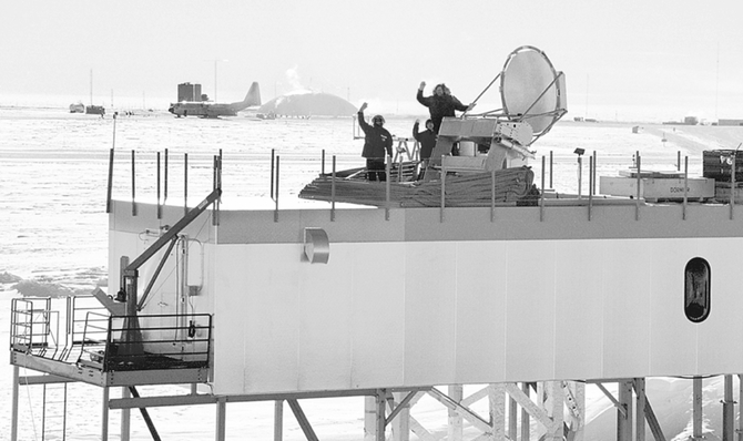
Fig. 1.— The Antarctic Submillimeter Telescope and Remote Observatory atop its building at the South Pole in 1997 February. Standing next to the telescope are G. Wright of Bell Labs and X. Zhang and A. Stark of Smithsonian Astrophysical Observatory. The telescope rests on a steel support tower which is structurally isolated from the building and can be covered by a fold‐off canopy made of canvas and aluminum tubing. The main part of the Amundsen‐Scott South Pole Station lies beneath the dome, which is about 1 km distant. An LC130 cargo aircraft is parked on the skiway. The South Pole itself is slightly below and to the right of the tail of the airplane. (Photo credit: A. Lane.)
This paper describes observing operations at AST/RO. A summary of logistical support requirements and measured site characteristics is given in § 2. The instrument and observatory facilities are described in § 3 and in Stark et al. (1997). Telescope pointing, calibration, and observing methods are described in § 4.
2. SITE CHARACTERISTICS
2.1. Logistics
The AST/RO telescope is located in the Dark Sector of the US NSF Amundsen‐Scott South Pole Station. The station provides logistical support for the observatory: room and board for on‐site scientific staff, electrical power, network and telephone connections, heavy‐equipment support, and cargo and personnel transport. The station power plant provides about 25 kW of power to the AST/RO building out of a total generating capacity of about 490 kW. The South Pole has been continuously populated since the first station was built in 1956 November. The current station was built in 1975, and new structures have been added in subsequent years to bring the housing capacity to 210 people in austral summer and 45 in austral winter. New station facilities are under construction and are expected to be operational by 2005. These include living quarters for a winter‐over staff of 50, a new power plant with greater generating capacity, and a new laboratory building.
Heavy equipment at the South Pole Station includes cranes, forklifts, and bulldozers; these can be requisitioned for scientific use as needed. The station is supplied by over 200 flights each year of LC130 ski‐equipped cargo aircraft. Annual cargo capacity is about 3500 tons. Aircraft flights are scheduled from late October to early February, so the station is inaccessible for as long as 9 months of the year. This long winter‐over period is central to all logistical planning for polar operations.
The SIS receivers used on AST/RO each require about 2 liters of liquid helium per day. As of mid‐2000, total usage of liquid helium at the South Pole averages 30 liters per day for all experiments. One or two helium‐filled weather balloons are launched each day. There is an ongoing loss of helium from the station, as it is used for a variety of experiments. The NSF and its support contractors must supply helium to the South Pole, and the most efficient way to transport and supply helium is in liquid form. Before the winter‐over period, one or more large (4000–12,000 liter) storage dewars are brought to the South Pole for winter use; some years this supply lasts the entire winter, but in 1996 and 2000 it did not. In 1998 December, no helium was available during a period scheduled for engineering tests, resulting in instrumental problems for AST/RO during the subsequent winter. The supply of liquid helium has been a chronic problem for AST/RO and for South Pole astronomy, but improved facilities in the new station should substantially improve its reliability.
Internet and telephone service to the South Pole is provided by a combination of two low‐bandwidth satellites, LES‐9 and GOES‐3, and the high‐bandwidth (3 Mbps) NASA Tracking and Data Relay Satellite System TDRS‐F1. These satellites are geosynchronous but not geostationary, since their orbits are inclined. Geostationary satellites are always below the horizon and cannot be used. Internet service is intermittent through each 24 hour period because each satellite is visible only during the southernmost part of its orbit; the combination of the three satellites provides an Internet connection for approximately 12 hours within the period 01:00–16:00 Greenwich local sidereal time. The TDRS link helps provide a store‐and‐forward automatic transfer service for large computer files. The total data communications capability is about 5 Gbytes per day. AST/RO typically generates 1–2 Mbytes per day. Additional voice communications are provided by a fourth satellite, ATS‐3, and high‐frequency radio.
At AST/RO, all engineering operations for equipment installation and maintenance are tied to the annual cycle of physical access to the instrument. Plans and schedules are made in March and April for each year's deployment to the South Pole: personnel on‐site, tasks to be completed, and the tools and equipment needed. Orders for new equipment must be complete by June and new equipment must be tested and ready to ship by the end of September. For quick repairs and upgrades, it is possible to send equipment between the South Pole and anywhere serviced by commercial express delivery in about 5 days during the austral summer season.
AST/RO group members deploy to the South Pole in groups of two to six people throughout the austral summer season, carry out their planned tasks as well as circumstances allow, and return, after stays ranging from 2 weeks to 3 months. Each year there is an AST/RO winter‐over scientist, a single person who remains with the telescope for 1 year. The winter‐over scientist position is designed to last 3 years: 1 year of preparation and training, 1 year at the South Pole with the telescope, and 1 year after the winter‐over year to reduce data and prepare scientific results. If there are no instrumental difficulties, the winter‐over scientist controls telescope observations through the automated control program OBS (see § 4), carries out routine pointing and calibration tasks, tunes the receivers, and fills the liquid helium dewars. If instrumental difficulties develop, the winter‐over scientist carries out repairs in consultation with AST/RO staff back at their home institutions and with the help of other winter‐over staff at the South Pole.
AST/RO is located on the roof of a dedicated support building across the aircraft skiway in the Dark Sector, a grouping of observatory buildings in an area designated to have low radio emissions and light pollution. The AST/RO building is a single story, 4 m × 20 m, and is elevated 3 m above the surface on steel columns to reduce snow drifts. The interior is partitioned into six rooms, including laboratory and computer space, storage areas, a telescope control room, and a Coudé room containing the receivers on a large optical table directly under the telescope.
2.2. Instrument Reliability
AST/RO is a prototype, the first submillimeter‐wave telescope to operate year‐round on the Antarctic plateau. As such, its operation has been an experiment, minimally staffed and supported, intended to demonstrate feasibility and to identify areas of difficulty. A unique challenge of South Pole operations is the lack of transport for personnel and equipment during the 9 month winter‐over period. Spare or replacement parts for most of the critical system assemblies have been obtained, shipped to the South Pole Station, and stored in the AST/RO building. In a typical year, failure occurs in two or three system subassemblies, such as a drive system power supply or a submillimeter‐wave local oscillator chain. Usually a repair or workaround is effected by the winter‐over scientist. There are, however, single points of failure which can cause the cessation of observatory operations until the end of the winter. Between 1995 and 2000, observations or engineering tests were planned for a total of 54 months, of which about half were successful. The most important cause of telescope downtime has been incapacitation of the single winter‐over scientist, resulting in 14 months of lost time. Failure of the liquid helium supply was responsible for a further 11 months of lost time. In future, both of these causes for failure will be substantially reduced. Starting in 2002, it is planned that AST/RO will field two winter‐over scientists. Beginning in 2003, the completion of a new liquid helium supply facility as part of the new South Pole Station modernization plan will eliminate single points of failure for the liquid helium supply.
2.3. Site Testing
The sky is opaque to submillimeter wavelengths at most observatory sites. Submillimeter astronomy can be pursued only from dry, frigid sites, where the atmosphere contains less than 1 mm of precipitable water vapor (PWV). Water vapor is usually the dominant source of opacity, but thousands of other molecular lines contribute (Waters 1976; Bally 1989) a dry air component to the opacity. Chamberlin & Bally (1995), Chamberlin, Lane, & Stark (1997), and Chamberlin (2001) showed that the dry air opacity is relatively more important at the South Pole than at other sites. Dry air opacity is less variable than the opacity caused by water vapor and therefore causes less sky noise.
Physical parameters of the South Pole site of AST/RO are given in Table 1. The South Pole meteorology office has used balloon‐borne radiosondes to measure profiles above the South Pole of temperature, pressure, and water vapor at least once a day for several decades (Schwerdtfeger 1984). These have typically shown atmospheric water vapor values about 90% of saturation for air coexisting with the ice phase at the observed temperature and pressure. The PWV values consistent with saturation are, however, extremely low because the air is dessicated by the frigid temperatures. At the South Pole's average annual temperature of −49°C, the partial pressure of saturated water vapor is only 1.2% of what it is at 0°C (Goff & Gratch 1946). Judging by other measures of PWV such as LIDAR and mid‐infrared spectroscopy, the calibration of the hygrometers used on balloon sondes was accurate between 1991 and 1996. On 1997 February 22, the balloon radiosonde type was changed from an A.I.R. Model 4a to the A.I.R. Model 5a, and the average PWV values indicated by the new radiosondes dropped by 70% (see Fig. 2); these new values appear to be spuriously low. A firm upper limit to the PWV can be set by calculating what the PWV would be if the column of air were 100% saturated with water vapor at the observed temperature and pressure, the saturation‐point PWV. Since the temperature and pressure measurements from balloon sondes are accurate, and since the atmosphere cannot be significantly supersaturated, the saturation‐point PWV is a reliable upper limit to the true PWV. Values of the saturation‐point PWV for a 38 year period are shown in Figure 3 (Chamberlin 2001). Figure 4 shows the PWV for each day of the year averaged over all the years in this data set to show the average seasonal variation in the water vapor content of the atmosphere. PWV values at the South Pole are small, stable, and well understood.

Fig. 2.— Balloon measurements of PWV at the South Pole. (Left) Quartiles of precipitable water vapor (PWV) distribution in winter (day of year 100–300) from 1991 through 1998, calculated from balloon‐borne radiosonde measurements. The radiosonde type was changed in early 1997, and the subsequent calibration has been spurious. This new radiosonde, the AIR model 5a, has been used in measurements at other sites, in particular the peaks surrounding Chajnantor plateau (Giovanelli et al. 1999); the 1997 South Pole measurements make possible a direct comparison. (Right) Quartiles of saturation‐point PWV distribution in winter (day of year 100–300) for 1992–1998, calculated from balloon‐borne pressure and temperature measurements. Saturation‐point PWV is calculated by assuming 100% water vapor saturation for a column of air with a measured temperature and pressure profile. Since temperature and pressure sensor calibration is more reliable than hygrometer calibration, this value gives reproducible results. If hygrometer measurements from 1991–1996 can be trusted, the winter South Pole atmosphere is, on average, 90% saturated.
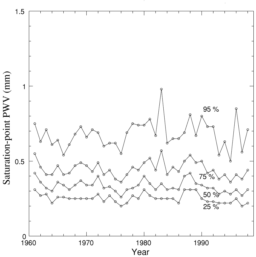
Fig. 3.— Saturation‐point PWV at the South Pole, 1961–1998, adapted from Chamberlin (2001). Quartiles of saturation‐point PWV distribution during the winter (day of year 100–300) for 1961–1998, calculated from balloon‐borne pressure and temperature measurements. This figure illustrates the long‐term stability of the South Pole climate.
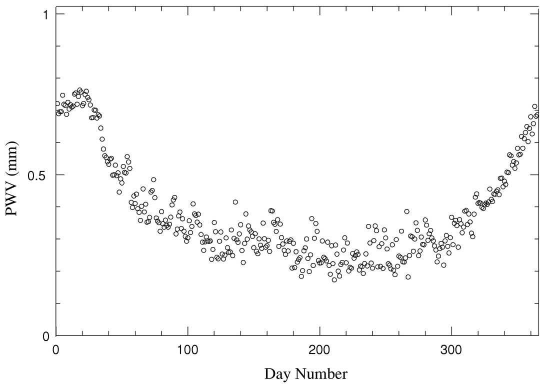
Fig. 4.— Average PWV at the South Pole by day of year, 1961–1999, adapted from Chamberlin (2001). The PWV in millimeters for each day of the year between 1961 and 1999 is averaged and plotted as a function of day of year. This plot shows the average seasonal trend, where the average water vapor content of the atmosphere declines from February through September.
 |
Quartile values of the distribution of PWV with time are plotted in Figure 5 (from Lane 1998), where they are compared with corresponding values for Mauna Kea and for the proposed Atacama Large Millimeter Array (ALMA) site at Chajnantor. The relation between PWV and measured opacity at 225 GHz (Hogg 1992; Masson 1994, S. Foster, private communication) was used to derive the PWV values for Mauna Kea and Chajnantor. Recent Fourier Transform Spectrometer results from Mauna Kea (Pardo, Serabyn, & Cernicharo 2001b) show that this PWV‐τ225 relation may overestimate PWV by about 12%. The data are separated into the best 6 month period and the remainder of the year. Of the three sites, the South Pole has by far the lowest PWV, during austral summer as well as winter.
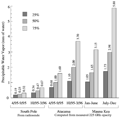
Fig. 5.— Quartiles of PWV at three sites, from Lane (1998). The South Pole is considerably drier than Mauna Kea or Atacama (Chajnantor). During the wettest quartile at the South Pole, the total precipitable water vapor is lower than during the driest quartile at either Mauna Kea or Atacama.
Millimeter and submillimeter‐wave atmospheric opacity at the South Pole has been measured using skydip techniques. Chamberlin et al. (1997) made over 1100 skydip observations at 492 GHz (609 μm) with AST/RO during the 1995 observing season. Even though this frequency is near a strong oxygen line, the opacity was below 0.70 half of the time during austral winter and reached values as low as 0.34, better than ever measured at any ground‐based site. The stability was also remarkably good: the opacity remained below 1.0 for weeks at a time. The 225 GHz (1.33 mm) skydip data for the South Pole were obtained during 1992 (Chamberlin & Bally 1994, 1995) using a standard NRAO tipping radiometer similar to the ones used to measure the 225 GHz zenith opacities at Mauna Kea and Chajnantor, and the results are summarized by Chamberlin et al. (1997) and Lane (1998). The tight linear relation between 225 GHz skydip data and balloon sonde PWV measurements is discussed by Chamberlin & Bally (1995).
From early 1998, the 350 μm (850 GHz) band has been continuously monitored at Mauna Kea, Chajnantor, and the South Pole by identical tipper instruments developed by S. Radford of NRAO and J. Peterson of Carnegie‐Mellon University (CMU) and CARA. Results from the South Pole are compared to Chajnantor and Mauna Kea in Figure 6. These instruments measure a broad band that includes the center of the 350 μm window as well as more opaque nearby wavelengths. The τ‐values measured by these instruments are tightly correlated with occasional narrowband skydip measurements made within this band by the Caltech Submillimeter Observatory and AST/RO; the narrowband τ‐values are about a factor of 2 smaller than those output by the broadband instrument. The 350 μm opacity at the South Pole is consistently better than at Mauna Kea or Chajnantor.
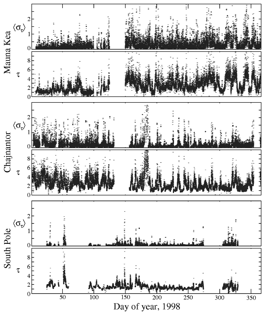
Fig. 6.— Sky noise and opacity measurements at 350 μm from three sites. These plots show data from identical NRAO‐CMU 350 μm broadband tippers located at Mauna Kea, the ALMA site at Chajnantor, and the South Pole during 1998. The upper plot of each pair shows 〈στ〉, the rms deviation in the opacity τ during a 1 hour period—a measure of sky noise on large scales; the lower plot of each pair shows τ, the broadband 350 μm opacity. The first 100 days of 1998 on Mauna Kea were exceptionally good for that site. During the best weather at the South Pole, 〈στ〉 was dominated by detector noise rather than sky noise. Data courtesy of S. Radford and J. Peterson.
The simulations shown in Figure 7 were made with the "atmospheric transmission at microwaves" (ATM) model (Pardo, Cernicharo, & Serabyn 2001a). They include all water and oxygen lines up to 10 THz and account for the nonresonant excess of water vapor absorption and collision‐induced absorption of the dry atmosphere according to the results of Pardo et al. (2001b). For the comparison we have plotted typical transmission profiles for the three sites calculated for wintertime 25% PWV quartiles. For the South Pole, we use 0.19 mm PWV (Lane 1998). For Mauna Kea and Chajnantor we use the values 0.9 and 0.6 mm, respectively. The collision‐induced nonresonant absorption of the dry atmosphere is higher at the South Pole owing to the higher ground‐level pressure compared with the other two sites. The much smaller PWV levels of the South Pole, however, make its total zenith submillimeter‐wave transmission considerably better than those of Chajnantor and Mauna Kea.
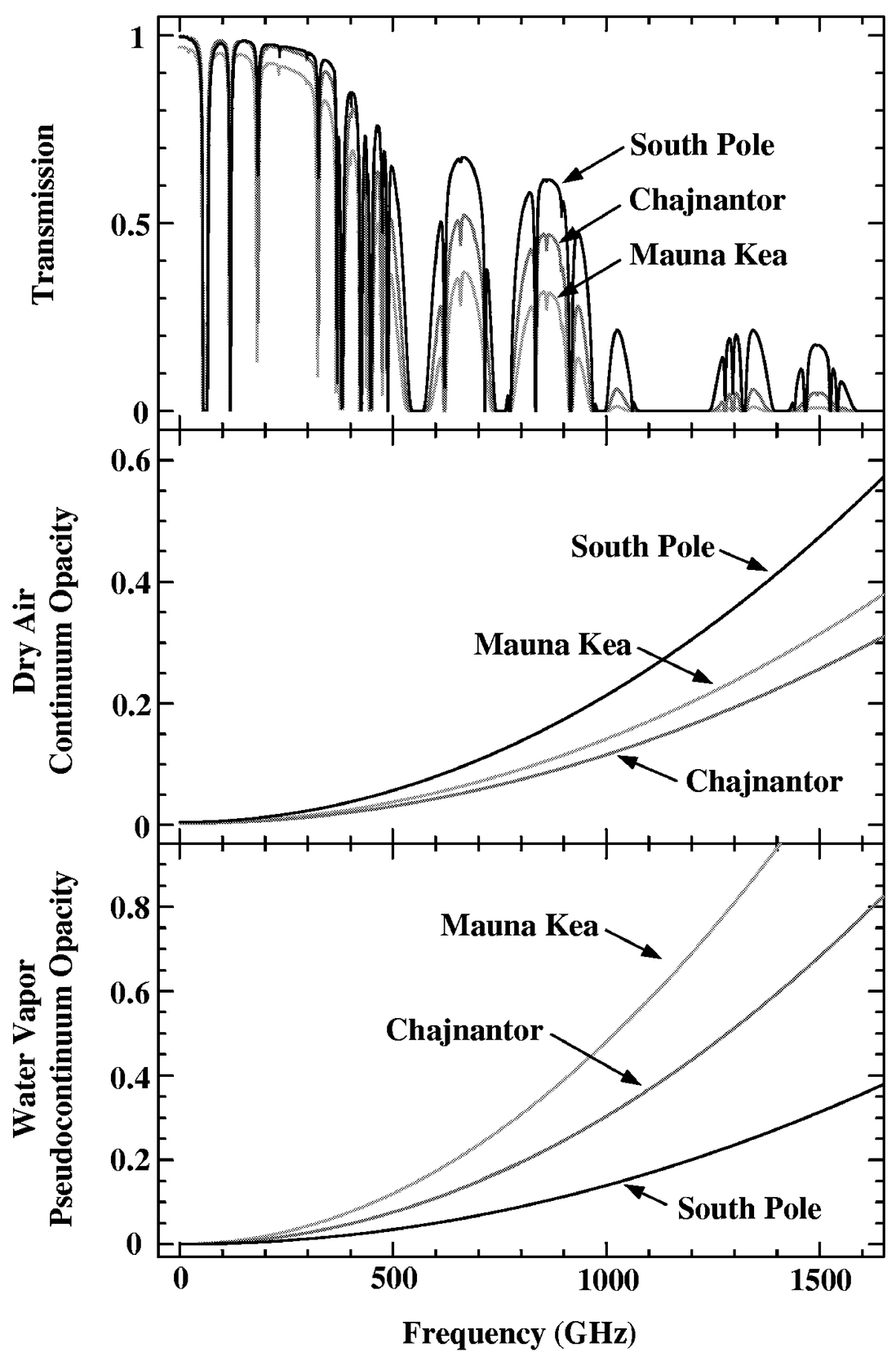
Fig. 7.— Calculated atmospheric transmittance at three sites. The upper plot is atmospheric transmittance at zenith calculated by J. R. Pardo using the ATM model (Pardo et al. 2001a). The model uses PWV values of 0.2 mm for the South Pole, 0.6 mm for Chajnantor, and 0.9 mm for Mauna Kea, corresponding to the 25th percentile winter values at each site. Note that at low frequencies, the Chajnantor curve converges with the South Pole curve, an indication that 225 GHz opacity is not a simple predictor of submillimeter‐wave opacity. The middle and lower plots show calculated values of dry air continuum opacity and water vapor pseudocontinuum opacity for the three sites. Note that unlike the other sites, the opacity at the South Pole is dominated by dry air rather than water vapor.
The success or failure of various submillimeter‐wave observational techniques depends critically on atmospheric opacity. Just as it makes no sense to carry out visual‐wavelength photometry in cloudy weather, there is an atmospheric opacity above which any particular submillimeter‐wave observational technique will fail to give usable results. This threshold depends on the details of the particular technique and its sensitivity to the spectrum of atmospheric noise, but for many techniques the threshold lies near τ∼1. Weather conditions above the threshold cannot be compared to those below the threshold by simple Gaussian noise analysis: 10 days where τ ≈ 1.5 can never be the equivalent of 1 day where τ ≈ 0.5. For deep background experiments, it is important to choose the best possible site.
Sky noise refers to fluctuations in total power or phase of a detector caused by variations in atmospheric emissivity and path length on timescales of order 1 s. Sky noise causes systematic errors in the measurement of astronomical sources. In an instrument that is well designed, meaning that it has no intrinsic systematic noise (see, for example, Kooi et al. 2000), the sky noise will determine the minimum flux that can be observed, the flux below which the instrument will no longer "integrate down." This flux limit is proportional to the power in the sky noise spectral energy distribution at the switching frequency of the observing equipment. Lay & Halverson (2000) show analytically how sky noise causes observational techniques to fail: fluctuations in a component of the data due to sky noise integrate down more slowly than t-1/2 and will come to dominate the error during long observations. Sky noise is a source of systematic noise which is not within the control of the instrument designer, and the limits to measurement imposed by sky noise are often reached in ground‐based submillimeter‐wave instrumentation.
Sky noise at the South Pole is considerably smaller than at other sites at the same opacity. As discussed by Chamberlin & Bally (1995) and Chamberlin (2001) and shown in Figure 7, the PWV at the South Pole is often so low that the opacity is dominated by the dry air component; the dry air emissivity and phase error do not vary as strongly or rapidly as the emissivity and phase error due to water vapor. The spectral energy density of sky noise is determined by turbulence in the atmosphere and has a roughly similar spectral shape at all sites (Lay & Halverson 2000). Measurement of spectral noise at one frequency can therefore be extrapolated to other frequencies.
Figure 6 gives a direct indication of sky noise at submillimeter wavelengths at the largest timescales. The value 〈στ〉 is the rms deviation of opacity measurements made within an hour's time. As a measure of sky noise, this value has two defects: (1) during the best weather it is limited by detector noise within the NRAO‐CMU tipper (which uses room‐temperature bolometers) rather than sky noise, and (2) the ∼10−3 Hz fluctuations it measures are at much lower frequencies than the switching frequencies used for astronomical observations. Therefore, 〈στ〉 is an upper limit to sky noise at very low frequencies; Figure 6 nevertheless gives a clear indication that the power in sky noise at the South Pole is often several times less than at Mauna Kea or Chajnantor.
Other instruments are sensitive to sky noise at frequencies near 10 Hz and can be used to give quantitative results over more limited periods of time. Sky noise at the South Pole has been measured in conjunction with cosmic microwave background experiments on Python (Alvarez 1995; Dragovan et al. 1994; Ruhl et al. 1995; Platt et al. 1997; Coble et al. 1999) and White Dish (Tucker et al. 1993). Python, with a 2 75 throw, had 1 mK Hz−1/2 sky noise on a median summer day, whereas White Dish, with a 05 throw, was much less affected by sky noise. Extrapolating to 218 GHz and a 02 throw, the median sky noise is estimated to be 150 μK Hz−1/2 even in austral summer, lower by a factor of 10 than the sky noise observed during Sunyaev‐Zeldovich (S‐Z) effect observations on Mauna Kea (Holzapfel et al. 1997).
Lay & Halverson (2000) have compared the Python experiment at the South Pole with the Site Testing Interferometer at Chajnantor (Radford, Reiland, & Shillue 1996; Holdaway et al. 1995). These are very different instruments, but the differences can be bridged by fitting to a parametric model. Lay & Halverson (2000) have developed an atmospheric model for sky noise with a Kolmogorov power law with both three‐ and two‐dimensional regimes and have applied it to data from Python and the Chajnantor Testing Interferometer. They find that the amplitude of the sky noise at the South Pole is 10–50 times less than that at Chajnantor. Sky noise at the South Pole is significantly less than at other sites.
The best observing conditions occur only at high elevation angles, and at the South Pole this means that only the southernmost 3 steradians of the celestial sphere are accessible with the South Pole's uniquely low sky noise—but this portion of sky includes millions of galaxies and cosmological sources, the Magellanic Clouds, and most of the fourth quadrant of the Galaxy. The strength of the South Pole as a submillimeter site lies in the low sky noise levels routinely obtainable for sources around the south celestial pole. This is crucial for large‐scale observations of faint cosmological sources observed with bolometric instruments, and for such observations the South Pole is unsurpassed.
3. INSTRUMENT AND CAPABILITIES
The instrumental design of the AST/RO telescope is described in Stark et al. (1997). This section describes the current suite of instrumentation and aspects of the telescope optics which affect observations.
3.1. Receivers
Currently, there are five heterodyne receivers mounted on an optical table suspended from the telescope structure in a spacious (5 m × 5 m × 3 m), warm Coudé room:
- 1.A 230 GHz SIS receiver, 55–75 K double‐sideband (DSB) noise temperature.
- 2.A 450–495 GHz SIS waveguide receiver, 200–400 K DSB (Walker et al. 1992).
- 3.
- 4.A 800–820 GHz fixed‐tuned SIS waveguide mixer receiver, 950–1500 K DSB (Honingh et al. 1997).
- 5.An array of four 800–820 GHz fixed‐tuned SIS waveguide mixer receivers, 850–1500 K DSB (Groppi et al. 2000, the PoleSTAR array).
A 1.5 THz receiver, TREND (Gerecht et al. 1999), and an imaging Fabry‐Perot interferometer, SPIFI (Swain et al. 1998), are currently in development.
3.2. Spectrometers
There are four currently available acousto‐optical spectrometers (AOSs):
- Two low‐resolution spectrometers (LRSs) with a bandwidth of 1 GHz (bandpass 1.6–2.6 GHz).
- An array AOS having four low‐resolution spectrometer channels with a bandwidth of 1 GHz (bandpass 1.6–2.6 GHz) for the PoleSTAR array.
- One high‐resolution AOS (HRS) with 60 MHz bandwidth (bandpass 60–120 MHz).
The LRSs are built with GaAs laser diodes at 785 nm wavelength operating in single mode at about 25 mW power. The HRS uses a 5 mW HeNe laser at 632 nm wavelength. The stability of these AOSs is high, with greater than 200 s Allan variance minimum time for the two LRSs and greater than 300 s for the HRS measured at the AST/RO site under normal operating conditions. The designs of these AOSs are very similar to the AOSs used at the KOSMA observatory (Schieder, Tolls, & Winnewisser 1989). All AOSs are set up for nearly full Nyquist sampling of the spectra, the pixel spacing of the LRS is 670 kHz at 1.1 MHz resolution bandwidth per pixel, while the HRS has 32 kHz pixel spacing at 60 kHz resolution bandwidth. The fluctuation bandwidth of the spectrometers, which is the effective bandwidth per channel appearing in the radiometer equation, is 50% larger than the resolution bandwidth. This is what is expected in a diffraction‐limited AOS design. Aside from a single failure of the HRS due to a faulty optocoupler chip, all the AOSs have been continuously operating for 5 years without any problem. Maintenance requirements have amounted to a check and test once a year. This AOS design is reliable, stable, and accurate.
3.3. Optics
All of the optics in AST/RO are offset for high beam efficiency and avoidance of inadvertent reflections and resonances. Figure 8 shows the optical arrangement in its Coudé form. The primary reflector is made of carbon fiber and epoxy with a vacuum‐sputtered aluminum surface having a surface roughness of 6 μm and an rms figure of about 9 μm (Stark 1995). The Gregorian secondary is a prolate spheroid with its offset angle chosen using the method of Dragone (1982), so that the Gregorian focus is equivalent to that of an on‐axis telescope with the same diameter and focal length. The diffraction‐limited field of view is 2° in diameter at λ = 3 mm and 20' in diameter at λ = 200 μm. The chopper can make full use of this field of view because it is located at the exit pupil and so does not change the illumination pattern on the primary while chopping.
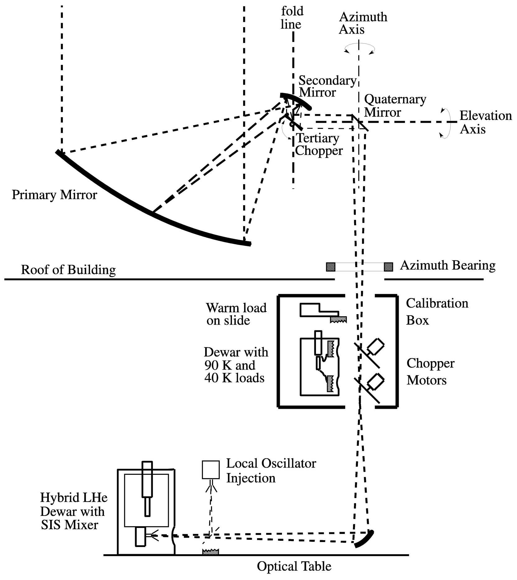
Fig. 8.— Schematic of the AST/RO optical system. For purposes of representation, the beam path has been flattened and the reader should imagine that the primary and secondary mirrors are rotated by 90° out of the plane of the page around the vertical "fold line." Note that rays diverging from a point on the primary mirror reconverge at the chopping tertiary mirror, since the tertiary is at the exit pupil of the instrument. The tertiary and quaternary mirrors are flat. The calibration loads are in a dewar to the side of the Coudé beam entering along the azimuth axis. The ambient temperature load is on a linear actuator and can slide in front of the sky port. Motorized chopper mirrors switch the receiver beam from the cooled loads to the sky or to the ambient temperature load.
Note in Figure 8 that rays diverging from a point on the primary mirror reconverge at the tertiary mirror, since the tertiary is at the exit pupil of the instrument. Optimizing the optics this way requires that the primary mirror be cantilevered away from the elevation axis: this is accomplished with a truss of invar rods which hold the primary‐to‐secondary distance invariant with temperature. When the fourth mirror shown in Figure 8 is removed, the telescope has a Nasmyth focus where the beam passes through an elevation bearing which has a 0.2 m diameter hole. Array detectors of various types can be used at this focus.
4. OBSERVING CONSIDERATIONS
Routine observations with AST/RO are automated, meaning that if all is well the telescope acquires data unattended for days at a time. The observing control language for AST/RO is called "OBS" and was developed over a 20 year period by R. W. Wilson and collaborators in order to automate operations on the Bell Laboratories 7 m antenna. OBS‐like languages are described by Stark (1993a, 1993b). OBS was modified for use on AST/RO by Huang (2001). With the installation of complex array instruments, the OBS language is evolving to accommodate a standard on‐the‐fly array instrument interface being developed for SOFIA, KOSMA, and the Heinrich Hertz Telescope. The signals controlled by OBS are shown in Figure 9. OBS commands and programs can be submitted via the computer network, and remote control of observations from sites beyond the South Pole Station network is possible during periods when communications satellites are available. For routine observations, winter‐over scientists normally monitor telescope operations from the living and sleeping quarters at the South Pole Station. This section describes aspects of the telescope and computer interface which should be considered by the observer. OBS commands for data acquisition and calibration are mentioned as appropriate.
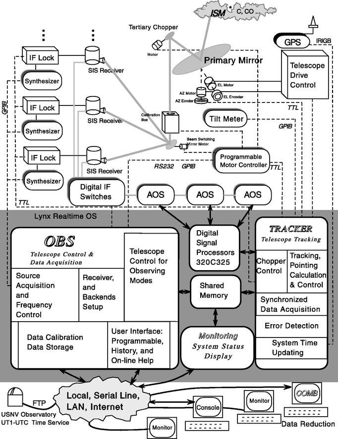
Fig. 9.— Schematic of the AST/RO control system (Huang 2001). This block diagram shows signal paths in the AST/RO system. Using a variety of interfaces and protocols, the computer monitors and controls the hardware subsystems to carry out the processes that constitute a radioastronomical observation. The data acquisition computer is shown as a shaded area.
4.1. Focus
The secondary mirror is mounted on a computer‐controlled positioning stage which allows the secondary mirror to be translated in three dimensions: a focus translation along the ray from the center of the primary to the center of the secondary, translation parallel to the elevation axis, and translation in a direction perpendicular to these two directions. The angular alignment of the secondary is not adjustable, but it does not need to be: as described in Stark et al. (1997), the primary mirror is aligned relative to the secondary mirror by mechanical means. This procedure sets the angular alignment. Figure 10 shows the horizontal and vertical beam sizes as a function of the focus adjustment, as measured by scans of the Sun. The data compare well with theoretical expectation near the point of best focus where the beam has a nearly Gaussian shape; the deviations between theory and measured points increase as the Gaussian approximation fails away from the point of best focus.
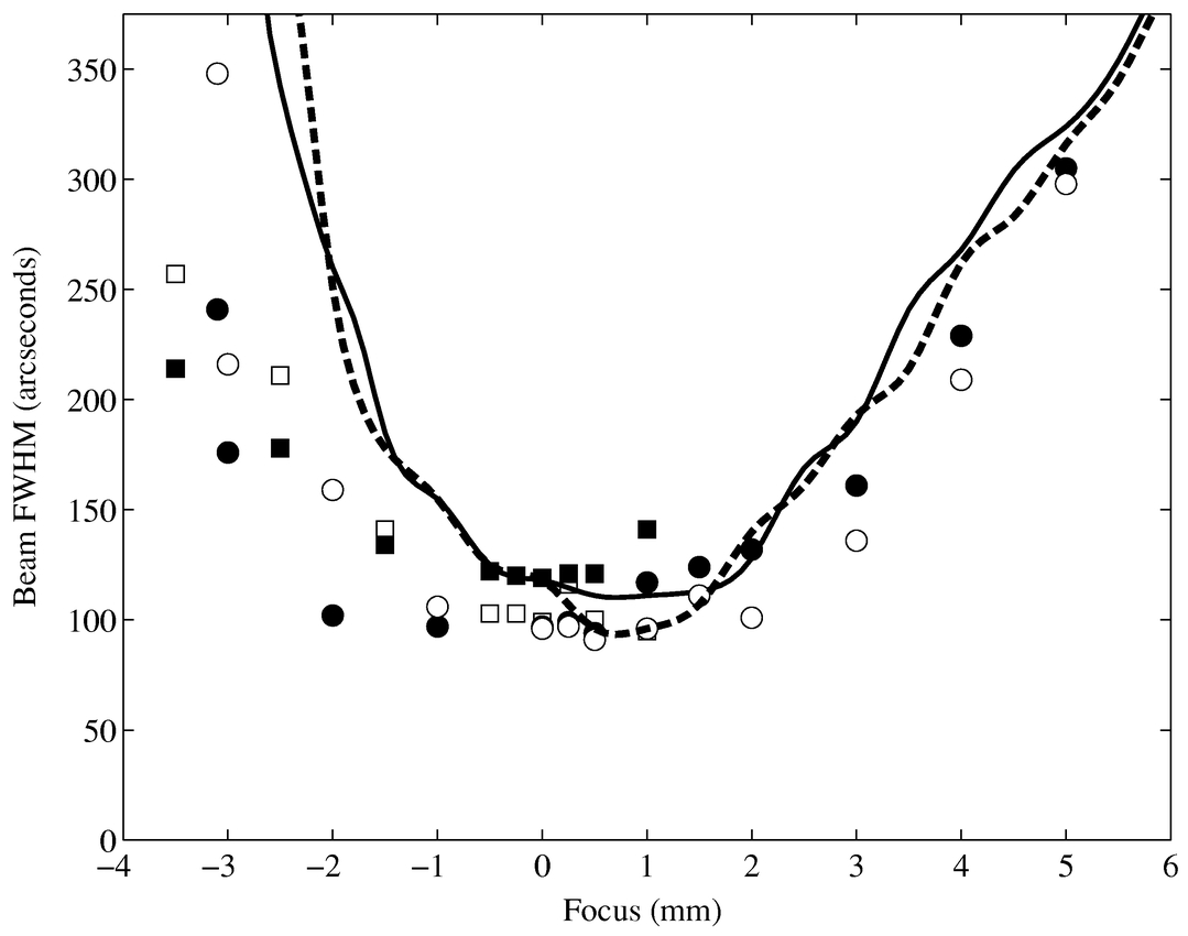
Fig. 10.— Theoretical and measured focus curves for AST/RO. The horizontal (filled symbols, solid line) and vertical (open symbols, dashed line) beam sizes are plotted as a function of focus adjustment. Positive focus adjustment moves the primary and secondary mirrors closer together. Data plotted as circles were obtained using the 460 GHz waveguide receiver; data plotted as squares were obtained using the 492 GHz quasi‐optical receiver. The solid and dashed lines represent results calculated from a model of the AST/RO optical system, assuming a 17.5 dB edge taper.
4.2. Optical Pointing
Telescope pointing is controlled by the main data acquisition computer, shown schematically in Figure 9. Input to the computer are time from the Global Positioning Satellite receiver and encoder readouts from both antenna axes. Output from the computer are the commanded velocities of the antenna axis motors. The commanded velocity is calculated from the difference between the encoder readouts and a command position, which is in turn calculated from the time, the telescope position required by the observing program, and the pointing model. The telescope drive system, as described in Stark et al. (1997), is a mostly analog electronic servo mechanism capable of driving the telescope so that the encoder reading differs from the position commanded by the computer by less than 1'' for antenna velocities near the sidereal rate. The pointing model characterizes the imperfections in the telescope construction, such as gravitational sag, bearing misalignments, and manufacturing errors.
4.2.1. Refraction
The pointing is corrected for refraction in the Earth's atmosphere by an approximate formula:

where n is the index of refraction,

where P is atmospheric pressure at the telescope, Pwater is the partial pressure of atmospheric water, and Tsurf is the atmospheric temperature at the Earth's surface (Bean 1962). The apparent elevation of sources is larger than it would be if the atmosphere were absent. At low frequencies, radio waves partially polarize atmospheric water vapor molecules, increasing the refraction compared to visual wavelengths. The third term in N, 3.75 × 10⁵(Pwater/1 mb)(1 K/Tsurf)2, is a manifestation of this effect—it represents the difference between visual and radio refraction. We assume that the term's coefficient, ξ(ν), is 1 while making submillimeter observations and 0 while making optical pointing measurements. This is a crude approximation, since ξ(ν) actually varies across the millimeter and submillimeter bands in a more complex manner which is not well characterized (Davis & Cogdell 1970). The errors introduced by this crude approximation are negligible for AST/RO, however, because the magnitude of the third term is small. The partial pressure of water vapor is never higher than 2 mb at the South Pole—this is the saturation pressure of water vapor (Goff & Gratch 1946) at the maximum recorded temperature of −14°C (see Table 1). The third term cannot therefore change the value of N by more than 6%; this corresponds to a difference between optical and radio pointing of 9'' at 20° elevation under worst‐case conditions. Equations (1) and (2) are approximate at the level of a few arcseconds (Seidelmann 1992, pp. 141ff.). Since sources do not change elevation at the South Pole, any residual errors tend to be removed by optical and radio pointing procedures.
The optical pointing model is determined by measurements of the positions of stars with a guide telescope mounted on AST/RO's elevation structure. The guide telescope consists of a 76 mm diameter, 750 mm focal length lens mounted at one end of a 100 mm diameter carbon fiber–reinforced epoxy tube and an Electrim EDC‐1000N CCD camera mounted at the other end on a focusing stage. The telescope tube is filled with dry nitrogen gas, sealed, warmed with electrical heater tape, and insulated. It works well under all South Pole conditions. In front of the lens is a deep red filter to facilitate detection of stars in daylight. Daylight observing capability is critical since the telescope is available to engineering and test teams only during the daylit summer months. The CCD camera is connected to a readout and control board in the data acquisition computer.
Following Condon (1992), the horizontal pointing error ΔAzcos (El) can be expressed as

where C1 is the optical telescope horizontal collimation error, C2 is the constant azimuth offset (encoder zero point offset), C3 represents the nonperpendicularity of the elevation and azimuth axes, C4 and C5 represent the tilt from vertical of the azimuth axis, and C6 through C9 represent irregularities in the bearing race of the azimuth bearing. The vertical pointing error ΔEl can be expressed as

where D1 is the optical telescope vertical collimation error plus encoder offset, D2 and D3 are mechanical sag and elevation encoder decentering, D4 and D5 represent the tilt from vertical of the azimuth axis, and D6 through D9 represent irregularities in the bearing race.
A pointing data set consists of position offsets (ΔAzi, ΔEli) as a function of (Azi, Eli), for several hundred observations of stars (i = 1,..., N). The ΔEli values are corrected for optical refraction by equations (1) and (2), with ξ(ν) = 0. The best‐fit values C1,..., C9 and D1,..., D9 in equations (3) and (4) are solved for as a function of the observed star positions and offsets. This is an inverse linear problem solved by standard numerical methods. The C1,..., C9 and D1,..., D9 constants are then inserted into the real‐time telescope drive system control software as corrections to the pointing. With this pointing model in place, subsequent observations of stars show errors of only a few arcseconds. This pointing process is repeated yearly. The high‐order terms, C6,..., C9 and D6,..., D9, have not changed significantly since they were first measured in 1993. The low‐order terms, C1,..., C5 and D1,..., D5, change because of instabilities in the mechanical mounting of the guide telescope, long‐term shifts in the telescope foundations, and thermal heating of the telescope tower during austral summer.
4.3. Radio Pointing
Implementation of the optical pointing mechanism assures that the optical telescope boresight attached to the telescope's elevation structure is pointed within specification. The radio receivers are, however, located at a Coudé focus, which is attached to the telescope mounting tower and fixed with respect to the Earth. As shown in Figure 8, the tertiary and quaternary steer the radio beam along the elevation and azimuth axes. Since the alignment of these mirrors is not perfect, additional corrections are needed for pointing each receiver (Zhang 1996).
In Figure 11, the elevation axis intersects the tertiary at O1 and the quaternary at O2. The intersection of the mechanical azimuth axis with the Coudé focal plane is point A. A photon traveling from O1 to O2 and then reflected from the quaternary will arrive at the focal plane at a point B. Point B and point A are not coincident because of misalignment of the quaternary mirror. If the tertiary is also misaligned, then the principal ray from the secondary will not coincide with the elevation axis. The principal ray reflects from the tertiary and quaternary and intersects the focal plane at a point whose position depends on the elevation angle, PEl. Figure 11 shows that the locus of points PEl describes a circle centered on point B. The three labeled points, P−90, P0, and P+ 90, show the intersection of the principal ray with the focal plane at elevation angles of −90°, 0°, and +90°. (Imagine that the elevation travel includes negative angles; in actuality the mechanical stops on AST/RO do not permit negative elevation angles.) Furthermore, when the telescope rotates around the azimuth axis, the points P−90, P0, P+ 90, and B precess around point A in a fixed pattern. We therefore see that a star on the boresight will have an offset from A given by

where the plus or minus sign in the elevation dependence is determined by the nature of the tertiary misalignment.
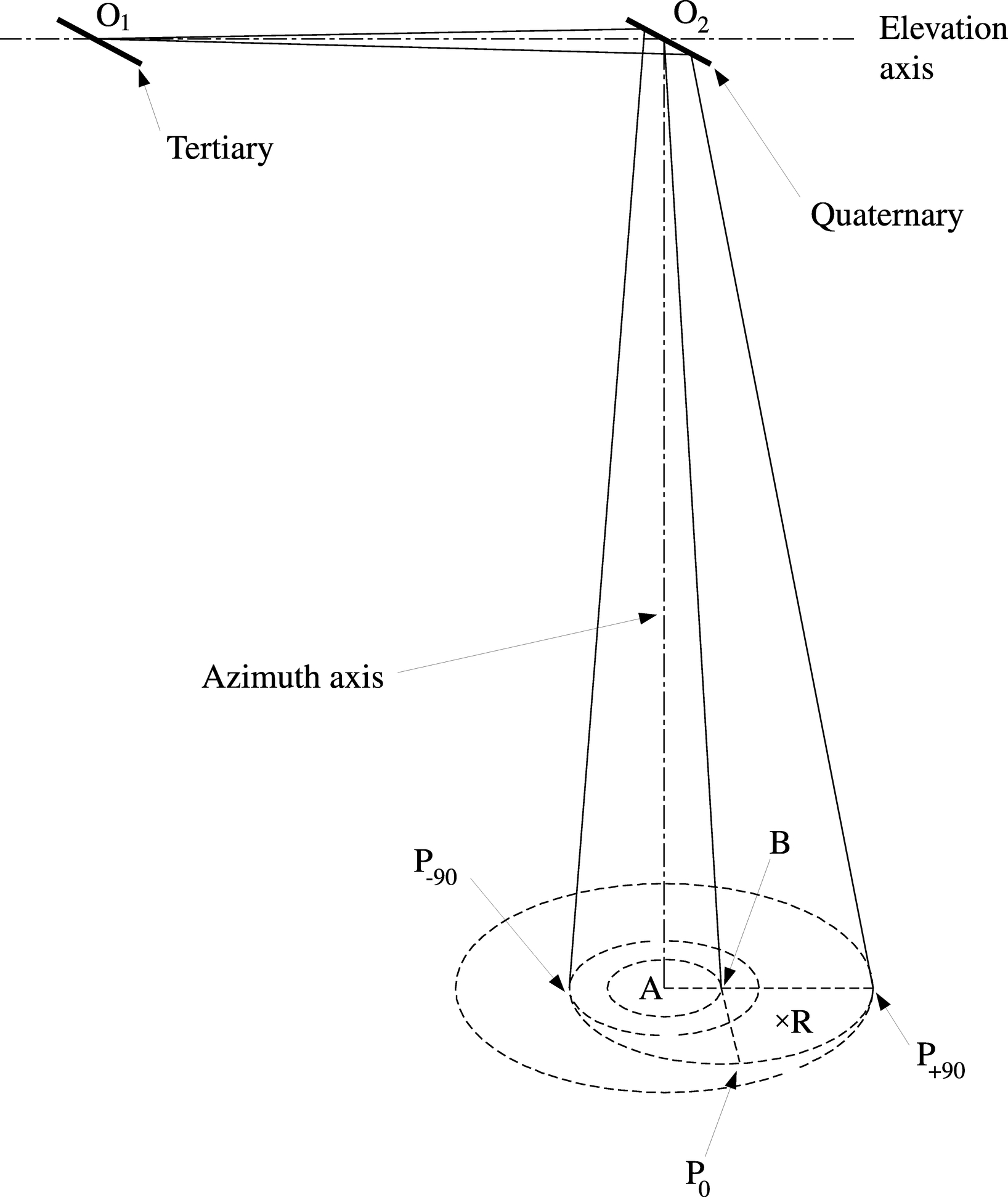
Fig. 11.— Geometry of AST/RO optics from the tertiary mirror to the Coudé focus (adapted from Zhang 1996). In general, the vectors AB→ and BP→+ 90 are not parallel, nor do they lie in the same plane as the azimuth and elevation axes.
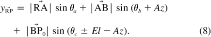
The receivers are not in general aligned with the azimuth axis, so let point R be the center of the receiver beamwaist at the Coudé focus. The image precession effect as viewed by the receiver is

where θa, θb, and θc are the phase angles of vectors RA→, AB→, and BP→0, respectively. The Cartesian components, x, y of the focal plane image viewed by the receiver change with the azimuth and elevation of the source as

These coordinates represent the point within the image plane of the Coudé focus which is observed by the receiver.
The radio beam pointing corrections modify the pointing of the telescope so that the nominal boresight falls on a particular receiver at all azimuth and elevation. These corrections are an inversion of the effect described by equations (7) and (8):


where A1ei θ1 corrects the error owing to the misalignment of the receiver, A2ei θ2 corrects the misalignment of the quaternary, and A3ei θ3 corrects for the combined misalignment of the primary, secondary, and tertiary plus any collimation offsets between the optical guide telescope and the radio beam. In this formulation, there are six constants and the unknown sign of the elevation dependence to be determined by fits to radio pointing data. As a practical matter, it is easy with AST/RO to obtain accurate radio data for a few bright sources at all azimuths, but known sources suitable for radio pointing are found only at a few elevations. Equations (9) and (10) are therefore modified to absorb the elevation dependence into the fitting constants:


For each elevation, a series of radio maps is used to determine the six parameters B1, B2, B3, B4, θ1, and θ2. If the mount errors have been correctly compensated for by equations (3) and (4), then B1 = B3 and θ1 = θ2. When these parameters are measured at several elevations, their value at all elevations is estimated by linear or quadratic interpolation in El. The magnitude of the pointing corrections given by equations (11) and (12) are typically 1'.
4.4. Chopper Offsets
As the chopper rotates, the beam position moves in both azimuth and elevation. Figure 12 shows the geometry of the beam position on the celestial sphere. When the chopper mirror is in its nominal, centered position, the radio beam points toward P0. When the chopper mirror rotates through an angle φ, the beam rotates through an angle 2ϕ and moves on the sky to point P1. The resulting change in elevation and azimuth can be calculated by considering the spherical triangle ZCP1, where Z is the zenith and C is the center of a small circle on the sky whose radius is the spherical angle RC. Solving for the arc ZP1, the spherical law of cosines gives
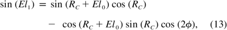
where El0 and El1 are the elevations of P0 and P1. The spherical law of sines gives
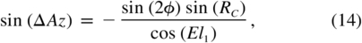
where ΔAz is the change in azimuth. These equations hold even if El0 + RC>90°, moving point C over the top to the other side of the zenith. In the AST/RO system, the value of φ is given by the encoder on the chopper motor. The value RC = 4 596 has been determined by measurements of the Moon and Sun. Figure 13 shows the beam size and displacement as a function of chopper angle.
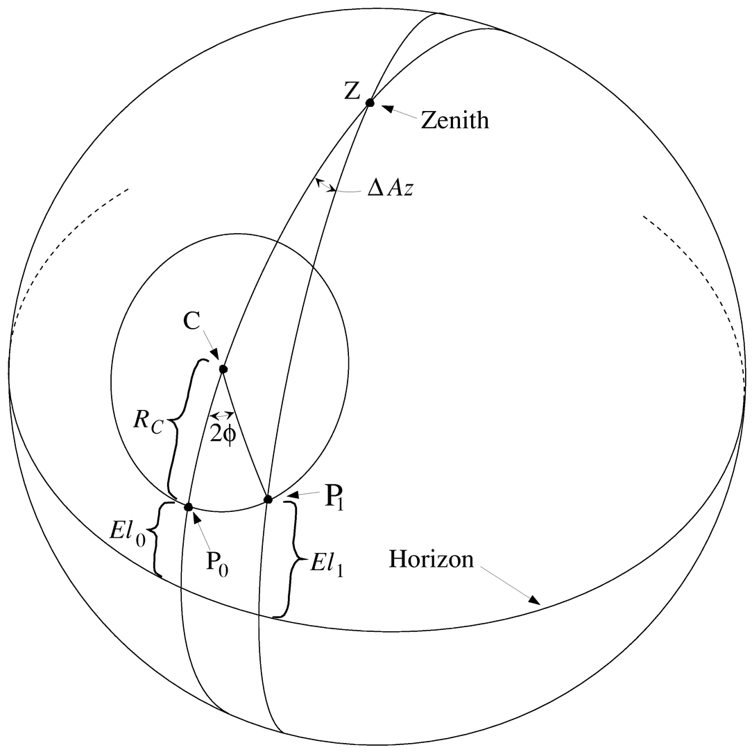
Fig. 12.— Geometry of AST/RO chopper motion on the celestial sphere. Point Z indicates the zenith of the celestial sphere, and point P0 is the direction of the telescope beam when the chopper is centered. When the chopper mirror rotates through an angle φ, the beam center moves to point P1 along a small circle centered at C. The radius of this circle is the spherical angle RC, whose value depends on the geometry of the optics.
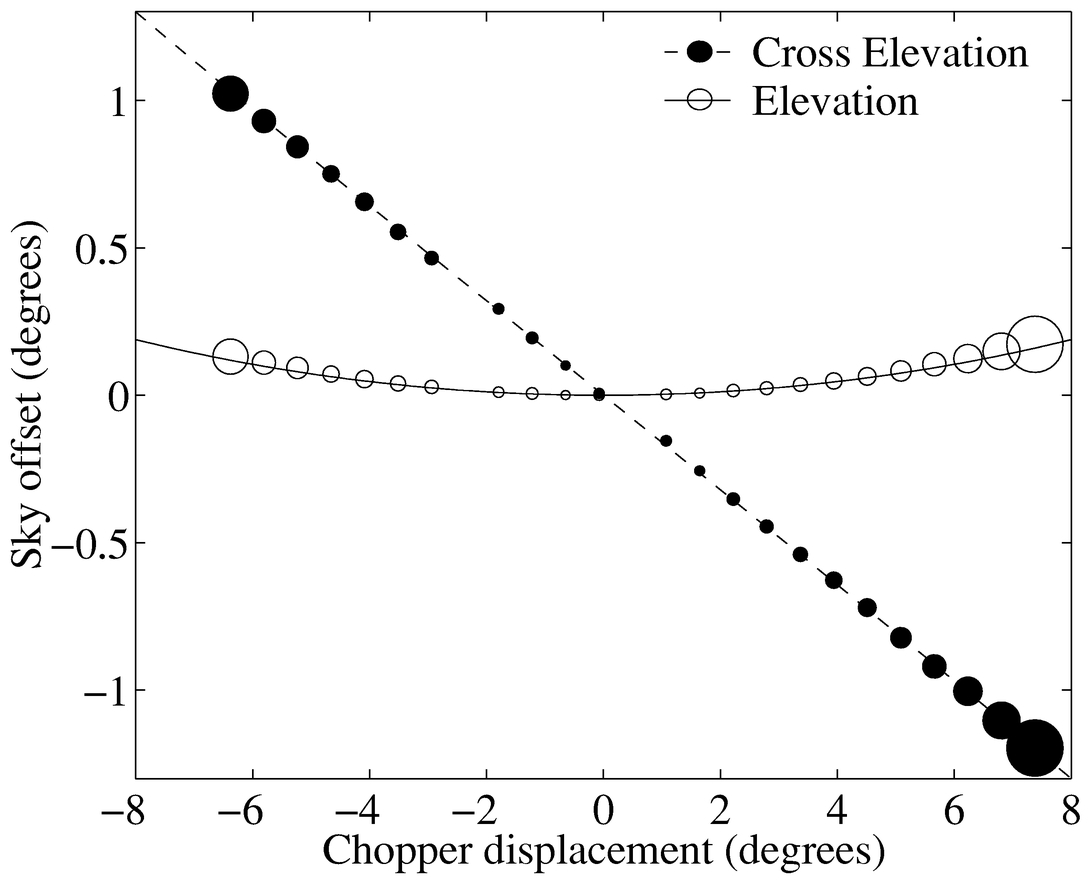
Fig. 13.— Measurements of the AST/RO chopper. Beam position is measured as a function of chopper displacement. Shown are elevation and cross‐elevation pointing offsets as a function of chopper motion. The ellipses represent beam size and position data measured during scans of the Sun at λ = 600 μm; each ellipse is similar in shape to the beam shape at that chopper displacement, and the size of each ellipse is given by the scale on the ordinate axis. The curves are calculations of the beam centroid based on a computer model of the optics.
4.5. Data Calibration
The real brightness temperature of an astronomical source depends only on the intrinsic radiation properties of the source, whereas the measured antenna temperature is influenced by the efficiency of telescope‐to‐source radiation coupling and the conditions in the Earth's atmosphere through which the radiation must propagate. Calibration converts from spectrometer output counts in the data acquisition computer to the source effective radiation temperature, correcting for atmospheric losses. The intermediate‐frequency (IF) output of a mixer in one of the AST/RO receivers is composed of downconverted signals from both the upper and lower sidebands. The amplified IF signal is detected by an AOS. The result is a spectrum of data with values proportional to the incident power spectrum. Discussed in this section is the conversion of these data values to the radiation temperature scale, T*R.
The chopper wheel method of calibration was originally described by Penzias & Burrus (1973) and elaborated upon by Ulich & Haas (1976) and Kutner & Ulich (1981). The theory of absolute calibration of millimeter‐wavelength data has not changed in its fundamentals since those papers were written, but the introduction of automated calibration loads at temperatures other than ambient has led to improvements in technique and a conceptual shift in the understanding of calibration parameters.
- 1.The ambient chopper‐wheel calibration method determined the relative gain of each spectrometer channel at the time of the chopper‐wheel measurement and later applied that gain to the switched astronomical data, assuming that it had not changed. Data quality is improved by measuring the relative gain during the acquisition of the astronomical data using the "(S - R)/R" technique, where S refers to the "on‐source" (or signal) measurement and R refers to an "off‐source" (or reference) measurement. Calibration of such a spectrum requires, however, determination of the atmosphere‐corrected system temperature, T*sys.
- 2.The receiver temperature, Trx, and sky temperature, Tsky, are distinct quantities measuring different sources of noise in the system. The former is a property of the instrument and under the control of the observer, while the latter is a property of the ever‐changing sky. Using the ambient chopper‐wheel method as originally formulated (Penzias & Burrus 1973), these two noise power levels cannot be determined independently, because there is only a single calibration load of known temperature; this means, for example, that it is not possible to determine whether a loss of observing sensitivity is caused by a problem with the receiver or an increase in atmospheric opacity. With multiple calibration loads, as in the AST/RO system, both of these quantities can be determined and the observing program modified as appropriate.
4.5.1. Relation between TA and TB
The antenna temperature for an astronomical source is defined as its brightness temperature in the Rayleigh‐Jeans limit. If a radio telescope observes a source of specific intensity Iν, the source brightness temperature TB at frequency ν is given by the Planck function,

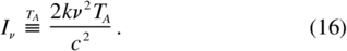
The blackbody emitter at temperature TB described by this equation is often fictitious—the usual circumstance for submillimeter observations of the interstellar medium is that the observed flux, Iν, results from thermal processes in emitters at temperatures higher than TB that do not fill the telescope beam or are not optically thick. The antenna temperature is given by the Rayleigh‐Jeans limit to equation (15),
The effective radiation temperature is

In the Rayleigh‐Jeans limit (hν/k≪T), Jν(T) = T; this approximation applies to essentially all temperatures within the AST/RO system, since h × 1 THz/k = 4.8 K, which is considerably lower than any physical temperature found in the AST/RO calibration system, telescope, or the atmosphere. It must be remembered, however, that the small flux levels of observed astronomical sources are expressed in the TA scale, which is simply defined to be proportional to power: TA = (c2/2kν2)Iν. This is a linear extrapolation to low power levels from the higher power levels of the calibration loads, where the calibration loads do satisfy the Rayleigh‐Jeans approximation at these frequencies. Setting equations (15) and (16) equal, we see that antenna temperature is the effective radiation temperature of the source brightness temperature,

but in general TA is small so that TB≳TA.
4.5.2. Calibration Scans
The AST/RO calibration system allows the receivers to "chop" between three blackbody loads and the sky (cf. Fig. 8 and Stark et al. 1997). There is a load at ambient receiver room temperature (the "warm" load) and two loads cooled by a closed cycle refrigerator to 40 K (the "cold" load) and 90 K (the "cool" load). The surfaces of the refrigerated loads are warmed to temperatures higher than their average physical temperature by infrared radiation entering the dewar windows, so that their effective radiation temperatures are about 100 K and 140 K, respectively. The effective radiation temperatures of the loads are measured about once a month by manually comparing the receiver response to each load with that of an absorber soaked in liquid nitrogen and to the warm load. The physical temperatures of all the loads are monitored by the computer, and we assume that if the physical temperature has not changed, the effective radiation temperature has not changed either.
During a calibration scan (performed via the OBS command ca), the data acquisition computer records data for each AOS channel corresponding to the receiver response to (1) no incoming IF signal (zero measurement), Dzero,j (this is essentially the dark current of the CCD output stage of the AOS), (2) the "cold" calibration load, Dcold,j, and (3) the "warm" calibration load, Dwarm,j. The "cool" load can optionally be used in place of either the "cold" or "warm" loads. It is best if the power levels of the receiver with the loads in place during calibration is similar to the power level while observing the sky. The AOS operates as a linear power detector; i.e., the spectrum of measured data values Dj is proportional to the incident power spectrum. For the jth AOS channel, we measure the gain:
The gains spectrum gives us the proportionality between the antenna temperature scale (TA) and the arbitrary intensity counts (D) read out from the AOS by the computer. The calibration spectrum measures the noise of the receiver, IF system, and AOS:
The average receiver noise temperature, 〈Trx〉, is the average of the calibration spectrum,
where the average is performed over a selectable subset of spectrometer channels.
4.5.3. The Single‐Slab Model of the Atmosphere
In the single‐slab model, the atmosphere is assumed to be a plane‐parallel medium with mean temperature Tat and double‐sideband zenith opacity τdsb. The sky brightness temperature can be expressed as (Chamberlin et al. 1997)

where we have introduced the spillover temperature, Tspill, the telescope loss efficiency, ηl, and A≡csc (El) is the air mass at the elevation of the telescope. The effective radiation temperature of the cosmic microwave background radiation is ignored because it is negligible at submillimeter wavelengths. The telescope loss efficiency, ηl, is the fraction of receiver response that originates from the sky. The spillover temperature, Tspill, is the effective radiation temperature of all sources of radiation incident on the receiver which are not from the direction of the sky. These sources primarily include the thermal emission from the optics and spillover from the Earth's surface. The quantity Tspill can be expressed as

where Tsbr is by definition the average temperature of the emitters giving rise to Tspill (Ulich & Haas 1976). Since there is a gradient in temperature between the air outside of the telescope and the warmed environment of the receiver room, Tsbr will fall somewhere between the outside surface temperature, Tsurf∼230 K, and the temperature of the receiver room, Twarm ≈ 293 K, depending on the quality of the receiver feed and its alignment.
4.5.4. Sky Brightness Measurement
The atmospheric attenuation of the signal is estimated by measuring the sky brightness temperature Tsky. The sky spectrum is made by measuring the sky and a cold load using the sk command in OBS. These are combined to yield

and averaging over channels gives
A skydip measures 〈Tsky〉 for a range of different elevations. These data can be fitted to the single‐slab model (eq. [22]) for the terms Tspill and τdsb and for the product ηlJν(Tat) (Chamberlin et al. 1997), which is used to determine ηl.
Instead of assuming that the mean atmospheric temperature, Tat, is equal to the ambient temperature, Tsurf, which is standard chopper‐wheel calibration procedure, we use actual in situ atmospheric measurements to deduce the mean atmospheric temperature. The South Pole meteorological station launches an upper‐air balloon once or twice each day to measure air temperature and relative humidity as a function of height. These data can be used to derive Tat, the mean atmospheric temperature in the column of air above the telescope. For each balloon flight in 1995 and 1996, we have approximated Tat at ν = 492 GHz by averaging the physical temperature of the atmosphere, T, over altitude, weighted by the opacity of seven nearby water lines:
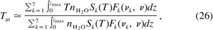
where nH2O is the density of water vapor at height z, νk is the frequency of water line k, Sk(T) is the line intensity of water line k, and Fk(νk, ν) is a Lorentzian line‐broadening function. During the South Pole winter, a temperature inversion occurs where the mean atmospheric temperature, Tat, is higher than the surface temperature, Tsurf. Figure 14 is a plot of Tat and Tsurf versus time for the year 1995. Despite the presence of this inversion layer for only part of the year, Tat is functionally related to Tsurf, with little scatter. Figure 15 shows Tat versus Tsurf for 1995, with a straight‐line fit to the data. The fit to the 1996 data is the same. Adopting the relationship

represents 90% of the data within ±4 K. Since Tat ≈ 230 K, this is a spread of only ±2%. Given a value of the surface temperature when a skydip measurement was made, this equation gives an estimate for Tat. The product ηlJν(Tat), fitted to skydip data, then gives an estimate of the telescope loss efficiency ηl. This procedure is most accurate during the best weather, when the fit to equation (22) is best. We assume that for a given configuration of the optics and receivers, ηl is constant and independent of the weather. Values of ηl on AST/RO have ranged from 0.65 to 0.92 for various alignments of the various receivers.
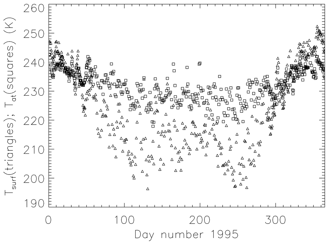
Fig. 14.— Tat and Tsurf vs. time at the South Pole (Ingalls 1999). Note the temperature inversion which occurs during the polar winter (Tat>Tsurf).
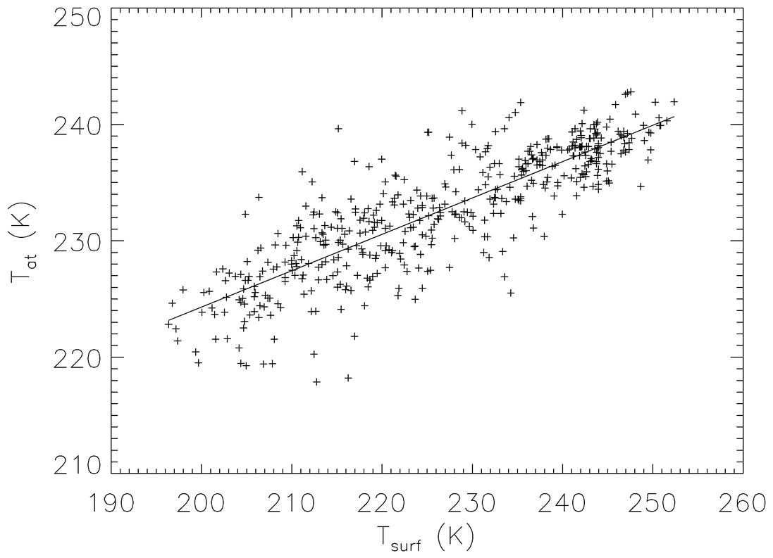
Fig. 15.— Tat vs. Tsurf at the South Pole (Ingalls 1999). The solid line shows the fit Tat = 0.31Tsurf + 162 K.
4.5.5. Single‐ and Double‐Sideband Atmospheric Opacity
For receiver systems with no method of sideband rejection, a given measurement is necessarily a double‐sideband measurement. In other words, the measured response of an AOS channel is a combination of two different frequencies, the signal sideband and the image sideband, possibly with different receiver gain in the two sidebands. The gains in the two sidebands are normalized so that gs + gi = 1. All of the current AST/RO receivers are double sideband, with gs≅gi≅1 /2.
A double‐sideband measurement of the sky brightness temperature is weighted by the gain, as well as the atmospheric opacity, in each sideband,

where τs and τi are the zenith opacities in the signal and image sidebands, respectively, and Tspill,s and Tspill,i are the spillover radiation temperatures at the frequencies νs and νi, respectively. Comparing equations (28) and (22), we see that we can use the skydip fitting method if


4.5.6. Spectral Line Measurements
The spectral line appears in only one of the sidebands. The source antenna temperature is a sum of contributions along the line of sight from both the source and the sky. Following Ulich & Haas (1976),
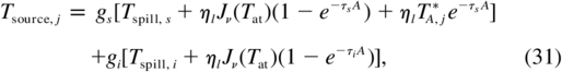
where T*A,j is the corrected antenna temperature of spectrometer channel j. Again, the cosmic microwave background radiation is ignored.
Observing always involves a switching scheme, where the frequency or position is changed and the signal on blank sky is subtracted from the signal on the source plus blank sky. In other words, subtracting equation (28) from equation (31) gives

or
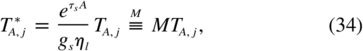
where M is the multiplier relating corrected and uncorrected antenna temperature. Skydips and sky temperature measurements yield τdsb, not τs. Substitution of equation (30) into equation (34) shows that
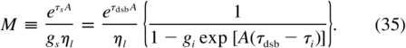
The term (τdsb - τi) is approximately constant in time and independent of PWV, since at most frequencies it is the dry‐air opacity which varies rapidly with frequency, whereas the water‐vapor pseudocontinuum opacity varies slowly with frequency (cf. Fig. 7). This term can therefore be treated as a constant correction term for a given tuning. One frequency and tuning at which this correction is particularly important is 492.1607 GHz C i, with the receiver‐tuned upper sideband so that the image sideband is near the oxygen line at 487.25 GHz. In this case, our 1.5 GHz IF frequency gives τdsb - τi≅ - 0.27.
In the AST/RO calibration system, the sky spectrum measurements are made several times each hour and are used to estimate the atmospheric opacity. Equations (22) and (23) can be rearranged to give
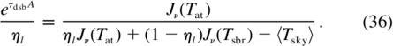
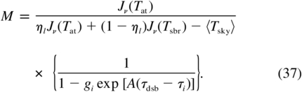
Since Tat ≈ Tsbr ≈ Tsurf, the denominator of this expression is essentially Tsurf - 〈Tsky〉, with corrections. When the opacity is high and M is large, as often occurs in submillimeter observations, these corrections are important. Note that the entire expression depends only weakly on ηl. We therefore see that M can be expressed in terms of known quantities:
For each spectrum, we define the atmosphere‐corrected system temperature as

where 〈Trx〉 has been determined by the most recent calibration and 〈Tsky〉 has been determined by the most recent sky brightness measurement at or near the elevation of the source. The atmosphere‐corrected system temperature is the noise power in a hypothetical perfect SSB telescope system above the Earth's atmosphere which has sensitivity equivalent to ours. The T*sys values for AST/RO vary from ∼200 K at 230 GHz to ∼30,000 K at 810 GHz, depending on receiver tuning and weather.
4.5.7. Spectral Line Data Acquisition
When observing the source, the average output of the jth channel of the spectrometer is

and when observing the reference, it is

These quantities can be combined using equation (32) to yield a measurement of the antenna temperature of the source:

where Tsky,j has been determined by the previous sky measurement (sk; eq. [24]) and Trx,j and Dzero,j have been determined by the previous calibration measurement (ca; eq. [20]).
A better quality spectrum can be obtained by replacing Tsky,j and Trx,j in equation (41) by their average quantities 〈Tsky〉 and 〈Trx〉, from equations (21) and (25):
This is because the actual noise power in the sky and from the receiver vary slowly across the bandpass of the spectrometer, whereas the calibration and sky spectra Trx,j and Tsky,j show spurious variations caused by reflections from the surfaces of the calibration loads and the windows of the calibration dewar. We then see from equations (34), (38), and (42) that

is the calibrated spectrum of the source. This is the "(S - R)/R" method of data acquisition. It provides a high‐quality spectrum of the source, because the gain of each channel, T*sys/(Dref,j - Dzero,j), is measured during the course of the observation.
In the AST/RO system, the data acquisition program OBS writes the values TA,j (usually calculated according to equation (42)—this is an option selectable by the observer) as scan data, and writes ηl, gs, El, 〈Tsky〉, 〈Trx〉, and Tsurf, together with about 50 other status variables, in the scan header. In the command gt in the data reduction program COMB, the multiplier, M, is calculated, and the data are converted to T*A,j.
The forward spillover and scattering efficiency, ηfss, is defined by Kutner & Ulich (1981) to be the fraction of the telescope's forward response which is also within the diffraction pattern in and around the main beam. This quantity relates T*A to the radiation temperature scale T*R, which is the recommended temperature scale for reporting millimeter‐wave data (Kutner & Ulich 1981): T*R = T*A/ηfss. The unusual optics of the AST/RO telescope (Fig. 8) give it feed properties similar to that of prime‐focus designs, for which ηfss ≈ 1.0 (Kutner & Ulich 1981). When the AST/RO beam, operating at 492 GHz, is pointed 4' from the Sun's limb, the excess T*A from the Sun is less than 1% of the brightness of the Sun's disk. This indicates 1.0≥ηfss>0.97, and so for AST/RO T*R = T*A × (1.015 ± 0.015).
5. CONCLUSION
AST/RO is the first submillimeter‐wave telescope to operate in winter on the Antarctic Plateau. During the first 5 years of observing, the most serious operational difficulties have been incapacitation of the single winter‐over scientist and lack of liquid helium—these problems are being addressed through allocation of additional resources, redundancy, and increased staffing. Site testing and observation have demonstrated that the South Pole is an excellent site having good transparency and exceptionally low sky noise. This observatory is now a resource available to all astronomers on a proposal basis.
Rodney Marks died while serving as the year 2000 AST/RO winter‐over scientist, and it is to him that this paper is dedicated. We thank Edgar Castro, Jeff Capara, Peter Cheimets, Jingquan Cheng, Robert Doherty, Urs Graf, James Howard, Gopal Narayanan, Maureen Savage, Oliver Siebertz, and Volker Tolls for their contributions to the project. Jonas Zmuidzinas has generously provided examples of his excellent SIS mixers. We also thank Rick LeDuc and Bruce Bumble at JPL for making SIS junctions and Tom Phillips at Caltech for making them available to us. We thank Eric Silverberg and the Smithsonian Submillimeter Array Project for the optical guide telescope. We thank Simon Radford of NRAO and Jeff Peterson of CMU for the data shown in Figure 6. We thank Juan R. Pardo of Caltech for discussions on atmospheric modeling and for carrying out the calculations shown in Figure 7. The AST/RO group is grateful for the logistical support of the National Science Foundation (NSF), Antarctic Support Associates, Raytheon Polar Services Company, and CARA during our polar expeditions. The University of Cologne contribution to AST/RO was supported by special funding from the Science Ministry of the Land Nordrhein‐Westfalen and by the Deutsche Forschungsgemeinschaft through grant SFB 301. This work was supported in part by US National Science Foundation grant DPP88‐18384, and by the Center for Astrophysical Research in Antarctica and the NSF under cooperative agreement OPP89‐20223.