
ABSTRACT
A small CCD photometer dedicated to the detection of extrasolar planets has been developed and put into operation at Mount Hamilton, California. It simultaneously monitors 6000 stars brighter than 13th magnitude in its 49 deg2 field of view. Observations are conducted all night every clear night of the year. A single field is monitored at a cadence of eight images per hour for a period of about 3 months. When the data are folded for the purpose of discovering low‐amplitude transits, transit amplitudes of 1% are readily detected. This precision is sufficient to find Jovian‐size planets orbiting solar‐like stars, which have signal amplitudes from 1% to 2% depending on the inflation of the planet's atmosphere and the size of the star. An investigation of possible noise sources indicates that neither star field crowding, scintillation noise, nor photon shot noise are the major noise sources for stars brighter than visual magnitude 11.6.
Over one hundred variable stars have been found in each star field. About 50 of these stars are eclipsing binary stars, several with transit amplitudes of only a few percent. Three stars that showed only primary transits were examined with high‐precision spectroscopy. Two were found to be nearly identical stars in binary pairs orbiting at double the photometric period. Spectroscopic observations showed the third star to be a high mass ratio single‐lined binary. On 1999 November 22 the transit of a planet orbiting HD 209458 was observed and the predicted amplitude and immersion times were confirmed. These observations show that the photometer and the data reduction and analysis algorithms have the necessary precision to find companions with the expected area ratio for Jovian‐size planets orbiting solar‐like stars.
Export citation and abstract BibTeX RIS
1. INTRODUCTION
A knowledge of other planetary systems that includes information on the number, size, mass, and spacing of the planets around a variety of star types is needed to deepen our understanding of planetary system formation and processes that give rise to their final configurations. Recent discoveries show that many planetary systems are quite different from the solar system in that they possess giant planets in short‐period orbits and that they often have highly eccentric orbits. Current theories predict that the size of the atmospheres of the short‐period planets will vary with the mass of the planet and the size of the orbital semimajor axis because of the intense stellar insolation. To obtain information on the size, mass, density, and orbital parameters of the giant inner planets and to develop the statistical dependencies of these, it is necessary to observe many of these objects for a variety of stellar spectral types and stellar compositions. Similarly, the discoveries that binary stars also have low‐mass companions (Cochran et al. 1997; Butler et al. 1997) demand that many more objects must be discovered and studied so that the differences between planetary systems of single stars versus multiple star systems can be understood.
The current method of discovering giant planets uses high‐precision Doppler velocity measurements of the shifting positions of a star's spectrum over a time interval of one to two planetary orbital periods. To detect planetary‐mass objects, the measurements of the wavelength shift must be made with a relative precision of a few parts per hundred million. To obtain this level of precision requires the photon shot noise to be extremely small, which, in turn, demands the use of very large aperture telescopes, such as the Keck instrument in Hawaii. Since only a few percent of the target stars show the presence of planets, this is a time‐consuming and expensive process. A much less expensive method of obtaining statistical information on inner planets is to use small photometric telescopes to identify those stars with planetary‐size companions and then determine their mass and density from Doppler velocity observations using a large‐aperture telescope. To test this approach, we have constructed a small photometer and have begun observations at the Lick Observatory on Mount Hamilton. This paper describes the photometer, provides a sampling of some stellar systems showing the presence of very low amplitude transits, and presents subsequent spectral and Doppler velocity observations of these stars.
2. PRECISION NEEDED TO FIND EXTRASOLAR PLANETS
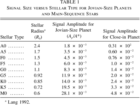
Transits of planets the size of Jupiter and Saturn produce a 1% reduction in the brightness of a G2 main‐sequence star like our Sun. For planets like 51 Peg B that are at distance of 0.05 AU from their star, the large heat flux from the nearby star is expected to prevent the contraction of gaseous planets so that the planetary radius could be as much as 1.9 times that of Jupiter (RJ) for a planet with an age of 1 Gyr or a value of 1.3RJ for a planet with an age of 8 Gyr (Guillot et al. 1996). Thus the signal from mature, close‐in planets is expected to be up to 70% larger than that from Jupiter. The expected signal amplitude for such planets also depends on the size of the star they orbit. For main‐sequence stars as large as spectral type F0, a Jovian‐size planet would produce a flux change of 0.45%. Flux reductions of 3% are expected for main‐sequence stars of spectral class M0. See Table 1.
 |
Signals with amplitudes of 1% or greater can be detected when special care is taken to minimize the errors introduced by the atmosphere and the instrumentation. Nevertheless, three or more transits that demonstrate a consistency in period, depth, and duration must be observed to have confidence in the reality of any detection. For sufficiently bright stars, the precision of ground‐based photometry is generally limited by atmospheric effects such as extinction and scintillation (Young 1974; Dravins et al. 1998), but it is also greatly affected by telescope tracking and by detector noise. On photometric nights and when sufficient care is taken, it is possible to obtain measurements with an hour‐to‐hour relative precision of 0.1%–0.3% (Olsen 1977; Frandsen, Dreyer, & Kjeldsen 1989; Gilliland & Brown 1992).
Note that in doing relative photometry, each target star is measured relative to a group of reference stars measured simultaneously with the target star and in the same field of view as the target star. The only measurements that we report here are the changes in the relative brightness of the target star (compared to its reference stars) that occur over a period of a few hours. The measurements of the relative brightness of all 6000 stars are repeated every 7.5 minutes throughout the night for every clear night during a period of several months. To avoid repositioning the photometer, only one star field is observed each 3 month period. By observing several transits and folding the data so that the transits align, we have been able to monitor many stars with an hour‐to‐hour relative precision of about 0.1%. Hence 10 σ detections are possible for Jovian‐size planets and 7 σ detections are expected for Saturn‐size planets.
3. EXPECTED DETECTION RATE
The expected detection rate per star can be estimated from

where Pd is the probability that a field star is a dwarf, Pp is the probability that a dwarf star has a planet with a 3–6 day orbit,Pa is the probability that the planetary orbit is aligned close enough to the line of sight to produce transits, and P3 is the probability that a star with a planet in an orbital plane on our line of sight will show three or more transits in the designated observation period.
For a given limiting magnitude, only about half the stars near the Galactic plane are dwarfs. Many of the rest are giants, which are too large to have short‐period planets or to show a detectable signal. Thus only one‐half of the field stars can be considered as targets, so Pd∼0.5.
Observations of solar‐like stars by Mayor & Queloz (1995), Butler et al. (1997), Cochran & Hatzes (1997), Noyes et al. (1997), and Marcy & Butler (1998) have shown that approximately 1%–2% of their target stars have giant planets with periods between 3 and 6 days (G. Marcy 1999, private communication). For those planets with orbital periods near 5 days, the probability that the orbital plane is near enough to our line of sight to show a transit is about 10%. (The slight increase in this fraction for the inclusion of planets with longer periods is ignored because of the small chance of observing the necessary three transits to recognize these events.) Hence Pp∼0.01 and Pa∼0.1.
The value of P3 was estimated from a numerical simulation. The simulation assumes that the observations were made for a constant number of hours each night and that no nights were lost to bad weather. Transits are placed at all possible phases for periods between 3 and 6 days. Then the fraction of events for which three or more transits occurred is recorded as a function of the number of nights of observations. The results are shown in Figure 1a. From this figure it can be seen that during the summer when nighttime durations average about 7 hours, nearly 6 weeks of observations are required to produce a 65% chance of detecting three or more transits by a star that is presenting transits. In the winter, the situation is much better in that 6 weeks of observations produce an 80% chance. Only star fields that are well away from the ecliptic can provide such long durations. Thus the product of probabilities (i.e., the probability that a given star will show at least three transits) varies from 3.2 × 10⁻⁴ in the summer to 4.0 × 10⁻⁴ during the winter.
Figure 1b shows that the actual probability is a function of the orbital period of the planet. For this calculation we used the actual data for the observations made in 1999 of the Cygnus star field. It is clear that for periods less than 4 days, the probability exceeds 0.9, and for orbital periods near 6 days, the fraction is near 0.7. These values are similar to those in Figure 1a for 8 weeks when the observations are conducted for 5–8 hours per night. Notice the large dips in the fraction of observable periods for integer and half‐integer values of the period in days.
The yield is defined to be the product of the probabilities times the number of stars monitored, i.e., about 1.9 and 2.4 planets when 6000 stars are monitored for 6 week periods during the summer and winter, respectively. For this calculation only the number of nights that are clear enough to achieve the required relative precision can be considered. Given the very real problems of bad weather and instrument downtime, this requirement often means that 2–3 calendar months will pass before the required number of nights is obtained. Nevertheless, observations of three rich star fields per year are practical. Thus about six planets should be discovered each year under these observing conditions.
4. INSTRUMENT DESCRIPTION
The Vulcan photometer is constructed from a 30 cm focal length, F/2.5 AeroEktar reconnaissance lens and Photometrics PXL16800 CCD camera. The lens is rigidly mounted in an aluminum box which also contains a digital micrometer stage that holds and moves the CCD camera as required for focusing. Figure 2 shows a design schematic of the photometer. A spectral bandpass filter is placed between the shutter and the front window of the detector. Mounted on the top of the photometer are two small finder telescopes and the autoguider with Celestron Pixel 255 CCD. See Figure 3.
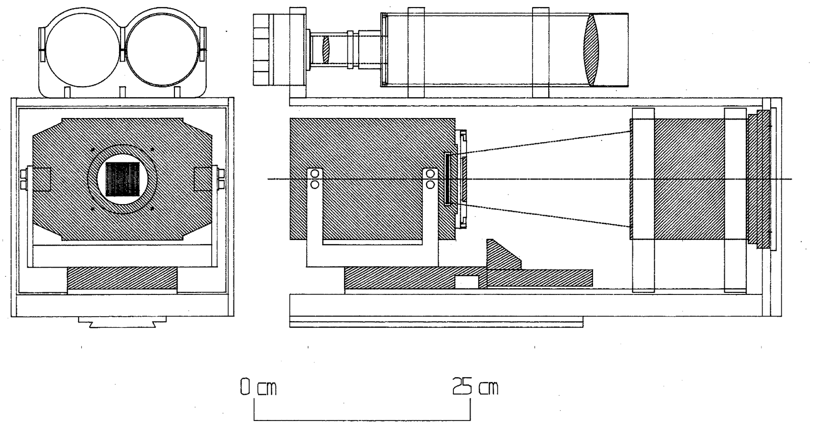
Fig. 2.— Schematic drawing of the Vulcan photometer
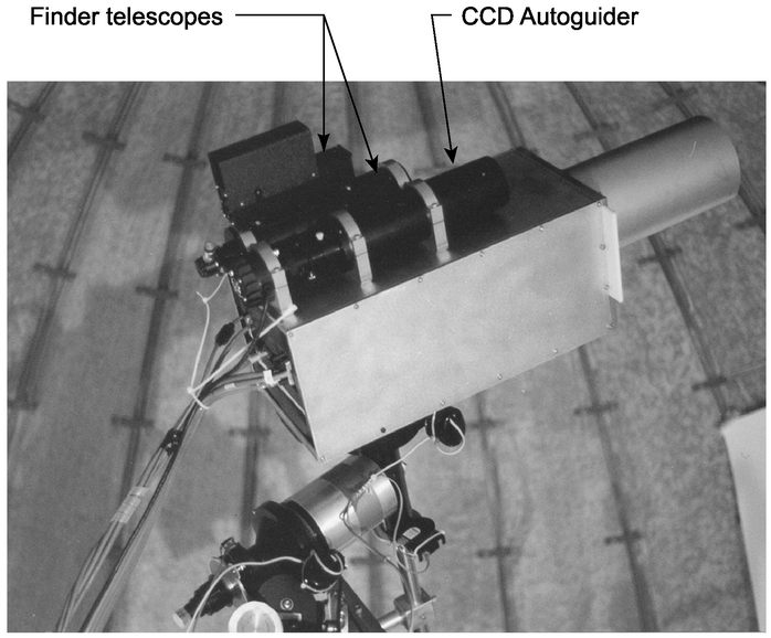
Fig. 3.— Photo of the Vulcan photometer in the Crocker Dome. At the top are two finder scopes and an autoguider. The white rectangle at the base of the tubular light baffle is the diffuser plate used for flat‐field calibration.
To minimize structural flexure and the differential motion between the autoguider and the main camera, the autoguider was built from a 8 cm aperture 30 cm focal length lens and 2× Barlow lens that gave an effective focal length of 0.6 m. Because the autoguider focal length is twice that of the main camera and because the autoguider pixels are 7 μm instead of 9 μm, autoguider errors of 1 pixel contribute less than 0.4 pixels to the motion of the star field on the main camera CCD. Thick brackets hold the short tube, Barlow lens, and the autoguider at three points along its length directly to the base plate. To avoid the necessity of flipping the telescope when it had crossed the meridian, the mounting was modified to move the telescope away from the pedestal and the counterweight was shifted toward the pedestal to balance the torque of the forward‐mounted camera.
A custom‐designed filter that covers the spectral range associated with both the V and R bands of UBVRI photometry was chosen to maximize the optical throughput while avoiding problems in the blue and red portions of the spectrum. The transmission curve is shown in Figure 4. At short wavelengths, there are rapid changes in extinction with changes in air mass that are mitigated by rejecting flux at wavelengths shorter than 480 nm. In the red portion of the spectrum, emissions from the sky background can be reduced by rejecting flux at wavelengths longer than 763 nm. The passband is also helpful in reducing the chromatic aberration of the AeroEktar lens.
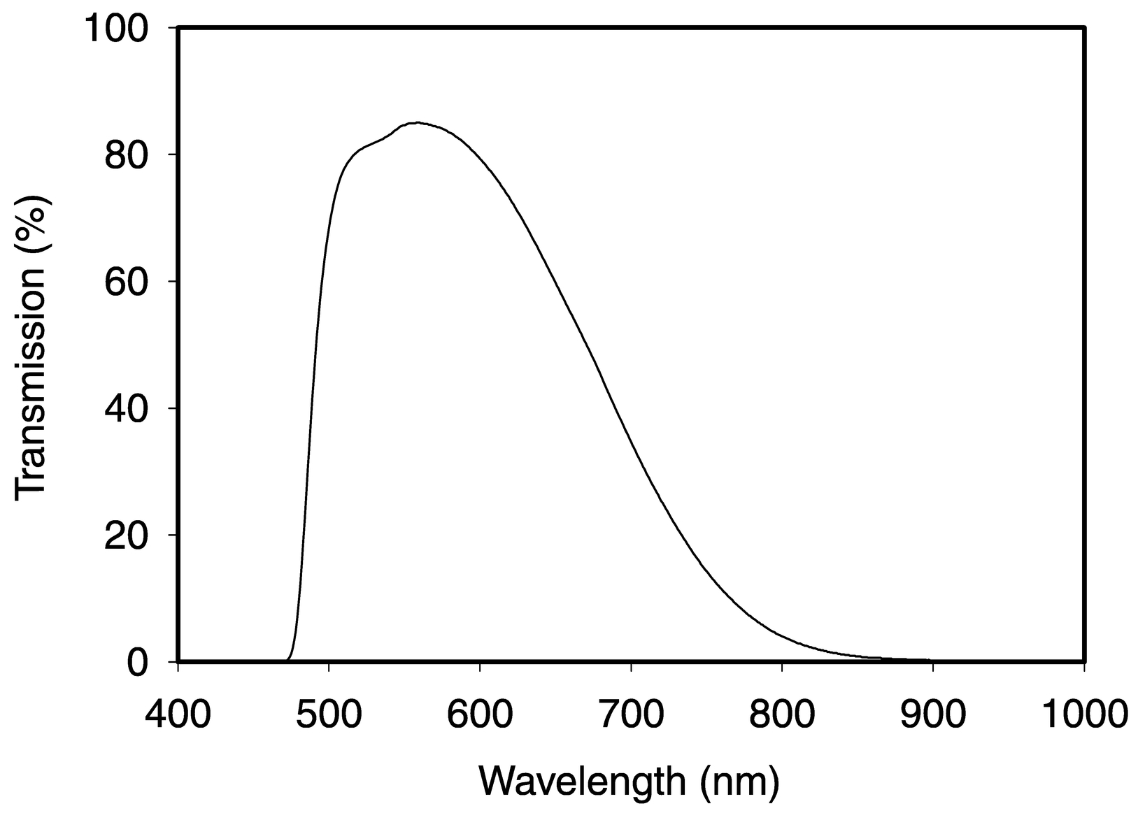
Fig. 4.— Transmission of the color filter
Measurements of the performance of the AeroEktar lens show that it transmits only about 45% of the incident light near 600 nm and that it has a point‐spread function (PSF) with very broad wings. Because the appropriate star fields are in the Galactic plane and are somewhat crowded, it is helpful to use a tighter PSF to avoid background stars and to minimize the noise introduced by the sky background. An study of the lens by T. Brown (1999, High Altitude Observatory, University Corporation for Atmospheric Research, personal communication) suggested that PSF could be improved without dramatically reducing the light in the star image by an aperture stop.
Figure 5 shows our measurements of the encircled energy as a function of image radius for the lens used in the Vulcan photometer for the full aperture lens and for the lens stopped to F3.8. Fifty percent of the flux is confined to a radius of 3.5 pixels (21'') for the lens stopped to F3.8, while the unstopped lens requires a 4.4 pixel (26 4) radius. Thus the stopped lens confines the flux to a core with ∼0.6 times the area of the unstopped lens. All data obtained after 1999 May 3 used the stopped lens. The large star images have the disadvantage of providing modest contrast against the background illumination from the sky. However, they are large enough to be oversampled and thereby accurately fitted by a PSF. Further, the PSF is not affected by seeing or changes in the seeing that occur during the night.
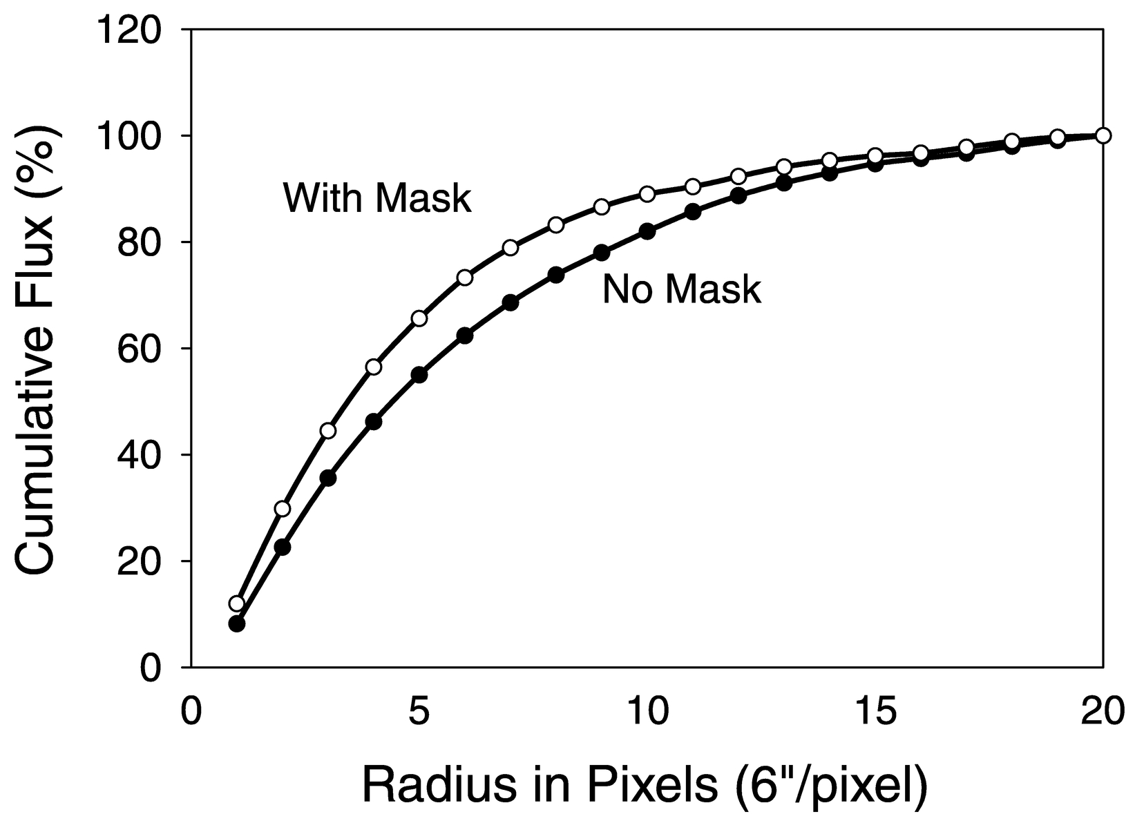
Fig. 5.— Effect of aperture mask on the encircled energy vs. image radius for the AeroEktar lens. Solid symbols represent the performance without a mask while the open symbols represent the effect of using an aperture mask.
The 49 deg2 field of view (FOV) that is obtained by using a 37 mm square CCD detector and a 300 mm focal length lens is very advantageous for simultaneously monitoring a large number of bright stars. Nevertheless, the FOV is so large that corrections for the scale changes and motions introduced by differential refraction must be done for each image before the photometry can be done. For example, in the Cygnus field, when the stars in the corner of the FOV nearest the horizon are at an air mass of 3, the differential refraction relative to stars in the center of the field is 27'' (4.5 pixels). For those stars at the other corner of the FOV, the change in relative position is 19'' (3.2 pixels). When the stars are near the meridian, the differential displacements at the corners shrink to about 5''. The small component of the image motion that can be represented by field rotation as the field moves from horizon to horizon is position dependent but is usually less than 2 pixels. Thus changes in the differential refraction cause significant and nonlinear plate scale changes throughout the night.
The CCD detector in the main camera is a Kodak 4096 × 4096 format front‐illuminated CCD with 9 μm pixels that is mounted in a Photometrics PXL 16800 camera. The detector is thermoelectrically cooled to −26.3°C ± 0.2°C. Because the data are read out as 16 bit numbers, each image file is 32 Mbytes in size. The large size of the files demands that the computer controlling the camera and recording the images use a 32 bit operating system and 32 bit software. Because of the rarity of 32 bit software to control the camera and to display and record the results, a beta version of "V" Software (of the Photometrics Corporation) is used. Exposures are 7.5 minutes long and include a 30 s period for reading out the data to hard disk storage. The exposure time is short enough to avoid saturating 9th magnitude stars but long enough to keep the amount of data to a manageable size. During an 8 hour night, about 2 Gbytes of data are recorded and then archived to CD‐ROMs. This data set includes files for dark, flat, and bias frames.
For calibration purposes, several exposures are made each evening and morning to measure the bias level, dark current, and flat‐field correction. The bias signal has been found to be nearly constant during a single night. Because the detector is run in the multipinned phase mode and because of the constant temperature maintained by the controller, the dark current is generally small and constant. As only a single exposure time is used for all the images, only one exposure time is needed for the dark current measurements.
Flat‐field calibrations are obtained by pointing the photometer toward a white diffuser screen attached to the dome and illuminated by a high‐temperature halogen lamp. To avoid focusing the white calibration screen onto the detector by the short focal length objective, a translucent diffuser plate is placed just in front of the lens.
The photometer is housed in the Crocker Dome on Mount Hamilton at Lick Observatory at an altitude of 1.3 km. The photometer is operated every clear night by a single member of a five‐person team. So that a large number of target stars can be observed simultaneously, star fields along the Galactic plane are monitored. A given field is monitored from dusk to dawn until several weeks of useful observations are acquired. This procedure provides maximum time coverage of the target stars and avoids wasted time due to slewing to new fields.
5. DATA PROCESSING
Because the goal of the Vulcan observations is the detection of extrasolar planets in inner orbits around dwarf stars, the methods employed to do the data analysis have been modified from the classical methods used in all‐sky photometry and for relative photometry. Standardized all‐sky photometry is best done by using photomultiplier tube detectors and special color filters and by comparing the target stars to standard stars. From such measurements, transformation coefficients are found that allow the transformation of the target star fluxes to those that would be measured with a "standard" system. When CCD detectors are used, accurate transformations to the standard system are very difficult. Further, Young et al. (1991) have shown that the equations upon which the transformations are based introduce significant errors. Relative photometry is less demanding in that the observations are made with reference to nearby stars of similar spectral characteristics rather than to the set of "standard stars." Since the comparison stars are chosen to be similar to the target star and to be nearby, correction for extinction is usually not needed.
Our goal does not require that we make an accurate2 determination of the brightness of stars relative to either standard stars or to nearby comparison stars, but requires only the measurement of the short‐term changes in the relative flux that occurs during a transit. We call our procedure "differential relative photometry" because of its similarity to relative photometry whereby the flux of a target star is measured relative to nearby comparison stars. Unlike the typical protocol used to do relative photometry, our method requires that corrections must always be made for extinction, and these must be measured for every star on every night. This is necessary because the amplitude of the flux change due to a transit is small compared to the flux change that occurs because of the continuously varying air mass. Since thousands of stars in the same field of view are measured simultaneously and observed for many nights, it is straightforward to do a flux versus time correlation to find appropriate comparison stars for each target star. The extinction correction for the target star is always based on those measured for the group of comparison stars known to have extremely similar extinction behavior.
However, there is no expectation that the same flux ratio of the target star to the group of comparison stars will be exactly the same from night to night. Small changes in the positions of the star images due to repositioning the telescope cause small changes in the output due to differing sensitivities of the individual pixels. These night‐to‐night changes are unimportant to the detection of the short transits that occur during a single night.
Since the transit periods sought are of the order of 3 hours, detection demands the measurements be made frequently throughout the night, but requires only that the relative precision of the photometry be maintained over a single night. Even if transits occur several nights or weeks apart, our goal can be attained without establishing and maintaining the accuracy required to measure the time‐invariant flux or flux ratio of the target and comparison stars. In this way, the method of differential relative photometry greatly reduces the need for long‐term stability and allows the emphasis to be placed on obtaining very high precision for hour‐to‐hour measurements.
Thus differential relative photometry differs from both all‐sky photometry and relative photometry in that it does not require the use of standard stars (because no transformations to a standard system will be made), but requires a high cadence of observations throughout the night, nightly measurements of extinction, and continuous observations of nearby comparison stars.
The data‐processing pathway for Vulcan camera images can be divided into several discrete steps: star field preparation, image calibration, image reduction, and transit detection. Each stage is dependent on results from the preceding steps, but otherwise can be carried out in any order, allowing for varying processing parameters or methods at any stage of the pipeline.
The first step is performed once for each star field. It consists of selecting stars to be monitored and preparing an initial catalog file of each star's position and brightness on a reference frame. The stars are located on a single low air mass image from a clear Moonless night. The image background is found by fitting a polynomial surface to median values of small subsections, each approximately 350 pixels on a side. The flattened image is then correlated with a model PSF, currently a weighted average of a night's worth of images for an isolated star. Because of variation of star PSFs across the image, the frame is divided into nine (3 × 3) subframes. The background‐subtracted subframes are each associated with a model PSF that is produced from the weighted average of all the images from a single night for an isolated star in the subframe. The result of this two‐dimensional correlation is a map of coefficients describing how well each point matches an isolated star. A threshold is applied to this map, and all adjoining pixels that have values above the chosen threshold are identified as a star.
When the threshold is found by demanding a correlation coefficient above 0.8, about 9500 stars are found in each of two Galactic plane fields. This method selects a subset of stars which have an isolated star PSF (i.e., no "significant" overlap from another star's PSF). Thus, even though most of the chosen target stars are in crowded star fields, the chosen targets are not crowded. Because nonstellar objects will also have a poor match to the standard PSF, they too are eliminated as targets. Stars that are near the edges of the CCD or near saturation are then eliminated from the list. Equatorial coordinates for the selected stars are determined from a third‐order plate transformation based on coordinates of known stars spread throughout the field. Results from this procedure consist of a list of star positions (both pixel row and column, and right ascension and declination), approximate visual magnitude, and catalog associations.
The second step is the generation of nightly and seasonal calibration images. We normally take several bias, dark, and flat frames each night. These images are combined to generate an average bias, dark, and flat for each night. We also create master calibration images from the average of all of the nightly files. These low‐noise images are used when there is little night‐to‐night variation in the calibration images.
The third step in the processing pipeline is the systematic reduction of images. Our reduction package processes all images from a single night at one time, but several nights can be done in batch mode. The steps taken in the reduction of a night's images to light curves are as follows:
- 1.Individual images are corrected with dark and flat images, and the pixel values are corrected for nonlinearity. The corrected frame is then registered with the reference frame to locate the target stars. The region around each target star that is large enough both to contain the star's PSF and to compute the background is saved to disk. This process is repeated for each image taken during the night.
- 2.For a small number of bright stars (of order 100), a PSF‐fitting algorithm is used to solve iteratively for a PSF model specific to each star. The subpixel position and brightness of each star in each frame is then determined. A second‐order coordinate transformation is fitted to the measured motions. Then the motion field is evaluated for each star to locate it on the data frame.
- 3.The interpolated motions are used to reduce the PSF‐fitting problem to a simple least‐squares problem, where the flux of each star in each frame is the only unknown parameter. The stars are then read into memory in batches of ∼100. The star images are checked for energetic particle hits and outlying images. Particle hits are found by locating positive spikes in the time series of each pixel. Pixel values above a given threshold are replaced with the value from a polynomial fit to the time series. The threshold and polynomial order were determined empirically but are user adjustable. Outlying star images are those for which the flux estimates differs substantially from the other estimates for that night. If outlying star images are found, they are flagged and not used in the PSF model for that star for that night. The star fluxes are fitted to the model PSF determined for each star from the night's images. The fluxes are then stored to disk along with supporting data including backgrounds, star positions and widths, and shot‐noise estimates for each star.
- 4.The raw fluxes generated in step 3 must be corrected for extinction. To get a first estimate of the out‐of‐atmosphere value for each star, the extinction coefficients for photometric nights are calculated from F(X) = F(0) × 10-αX, where F is the star flux, X is the air mass, and α is the extinction coefficient for each star. After removal of those stars found to have large night‐to‐night variations, comparison stars are found by computing the variance of the transmission difference between each nearby star and the target star for several photometric nights. The brightest 10 (nonsaturated) stars are then chosen for the ensemble. This procedure guarantees that only nonvariable stars with similar "color" are used as comparison stars. The average transmission determined on each frame for the 10 comparison stars is used to determine the out‐of‐atmosphere value for each target star.
- 5.Each star's extinction‐corrected flux is divided by the average of its extinction‐corrected comparison stars. A list of variable stars and stars which show a high level of scatter is kept for each star field. This list contains both stars that are truly variable and those that show significant variation on the night they were processed due to the presence of artifacts such as contamination due to light from aircraft and satellite overflights. These stars are not used in the extinction correction fit in step 4, nor in the differential photometry normalization.
The final step in the Vulcan data‐processing pipeline is an automated search of the light curves for transit signatures. Detecting transit signals is a classical signal detection problem for deterministic signals in colored noise (Van Trees 1968). Essentially, the optimal detector whitens the observations and then correlates the whitened data with the signal resulting from passing a transit through the same whitening filter. Folding the time series at the orbital period of a planet coherently adds the test statistics for the bin containing the transit. The test statistics add incoherently if the wrong period or bin is chosen. The detection rate depends on the signal‐to‐noise ratio (S/N) of a single event, the number of events, and the detection threshold.
The light curves are first processed to remove outliers and the effects of systematic errors that might otherwise perturb the results. Isolated outliers are identified by quantifying the effect of each sample on the variance of all the samples collected on the same night about a trend line fitted to the night's data. Individual samples contributing more than a user‐specified fraction of the night's variance are removed from the light curve. This process is iterated a few times. After isolated outliers are removed, systematic errors are detected and removed from the light curves by decorrelating each light curve against all other light curves over the entire data set using the procedure described in Jenkins et al. (2000). This technique removes structures that are highly correlated across multiple light curves while preserving structures that are unique to individual ones. The final step of preconditioning is the removal of an estimate of the mean flux for each night's observation from each light‐curve sample. Here the estimate used was the sample at the 60% position of all samples when the night's samples were ordered in ascending brightness. (The 50% sample represents the median of the set.) This choice tends to detrend light curves of eclipsing binaries and transits of 51 Peg–like planets better than the sample mean or median when the sample‐sample precision is much better than 1%. The resulting residual light curves are then subjected to a matched filter seeking transits with durations between 2 and 4 hours and periods between 1 and 12 days. The matched filter is implemented by convolving each light curve with a single prototype transit pulse and then folding the resulting single‐transit statistics at each trial period. The results are normalized by the standard deviation of the light curve and the square root of the energy of the periodic transit pulse, accounting for the effects of missing data. The maximum test statistic is recorded for each star, as well as the maximum single‐transit test statistic. The stars are ordered by the maximum test statistic in descending order for manual examination. In addition, a Lomb periodogram analysis is performed for each star to identify short‐period eclipsing binaries and other periodic variable stars as well as to provide additional information for the manual examination of the light curves. Light curves which have high maximum test statistics are then subjected to further scrutiny.
6. CURRENT DIFFERENTIAL RELATIVE PHOTOMETRIC PRECISION
To determine the differential relative photometric precision that can be obtained with the photometer, a star field in Cygnus was observed for several hours on a photometric night. The results are shown in Figure 6. The horizontal line (dotted) is an estimate of the maximum noise introduced by scintillation and is calculated (Young 1974; Dravins et al. 1998) for an air mass of 2.6. Because most observations are usually made at a much lower air mass, this value is an upper limit. The bottom curve (short‐dashed curve) is an estimate of the shot noise introduced by the background which must be subtracted from the stellar flux. For stars dimmer than visual magnitude 11.6, this adds a larger noise contribution than does the shot noise from the star itself. The high background level is caused by the large area (36 arcsec2) of the sky that is imaged onto each pixel by the short (30 cm) focal length camera lens. It would be an even greater noise source if the detector had larger pixels. The solid curve is an upper‐limit estimate of the total noise expected from all three noise sources.
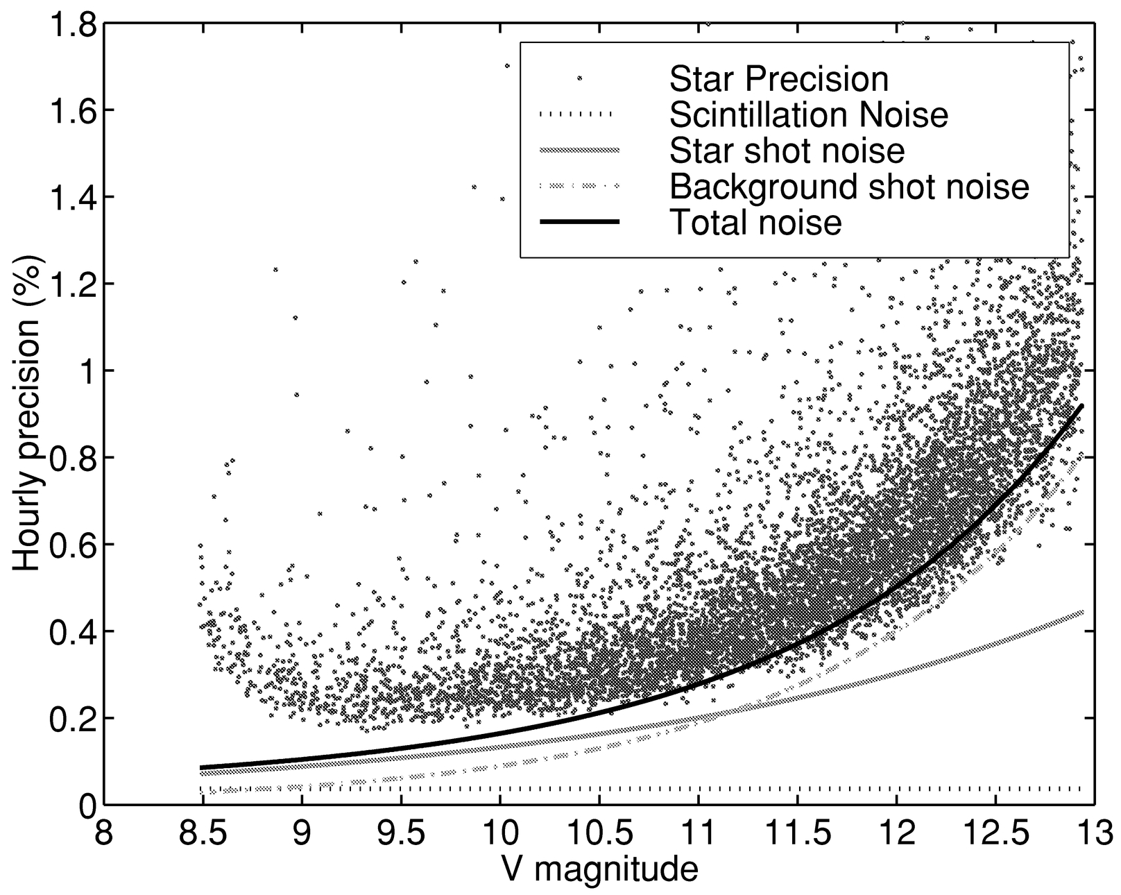
Fig. 6.— Measured and predicted precision vs. stellar magnitude. The upper solid curve represents the sum of the predicted scintillation and shot noise due to both the star and background. The lower solid curve represents the shot noise from the stellar flux, and the dash‐dotted curve shows the predicted shot noise from the sky background. The horizontal dotted curve is the predicted scintillation noise for an air mass of 2.6. Stars brighter than 9th magnitude have lower precision due to the presence of saturated pixels.
It is clear from a comparison of the data from predicted and measured precision for stars brighter than 11th magnitude that the noise introduced by the shot noise of the stars themselves is not a limitation; i.e., the small aperture is not the major limitation to the precision obtained here. Hence, another source of error must exist that is at least as important as those already discussed. An investigation was conducted to identify the other noise sources.
7. IDENTIFICATION OF PROCESSES THAT LIMIT PHOTOMETRIC PRECISION
Another potential source of noise is the overlapping of star images in the crowded fields. Because of the need to simultaneously monitor many stars, most of the chosen star fields are in, or close to, the Galactic plane.
A study was conducted of two portions of the Cygnus star field to determine if the measured photometric precision was related to the area density of stars, i.e., crowding. No significant correlation was found. This lack of correlation is probably due to the criterion that is applied to the original selection of target stars from the totality of the stars in the FOV of the reference frame. For a star to be selected as a target, it must show a good fit to a preselected PSF. This procedure eliminates overlapped stars, stars with bright neighbors, and nonstellar objects.
Small motions of an image across a CCD detector can cause large changes in the output because of the both intra‐ and interpixel variability (Buffington, Hudson, & Booth 1990; Buffington, Booth, & Hudson 1991; Robinson et al. 1995). Because of the potential importance of this noise source, extensive tests are underway to quantify the effect of image motions and to distinguish them from the effects of secular trends. It is also possible that the PSF‐fitting procedures are not adequate. (See the discussions in Howell 1989 and Stetson 1990.)
8. RESULTS OF EXAMINING THE LIGHT CURVES FOR 6000 STARS IN THE CYGNUS STAR FIELD
A 7° × 7° field centered at (R.A., decl.) = (19h47m, +36°55') was observed in 1998 from August 10 through September 30. Useful data were obtained on 29 nights. Nearly 50 stars showed some evidence of transits with periods between 0.3 and 8 days. Most had large amplitudes like the examples shown in Figures 7–10. Except for the very unlikely situation where the primary was later than spectral type M0, the amplitudes are too large to represent planetary transits. Further, the durations are also much longer than that expected from a planetary transit. The obvious presence of a secondary transit in all the figures confirms the multiplicity of the systems. Note that if the amplitudes of the primary and secondary transits in Figure 9 were slightly more equal, then it would be difficult to distinguish the two transits at half the real period from a single transit of a dark companion at that period. However, a small, dark companion can often be distinguished from two nearly identical stars that are showing grazing transits because of the V shape of the latter's transit compared to the nearly constant amplitude of the former.
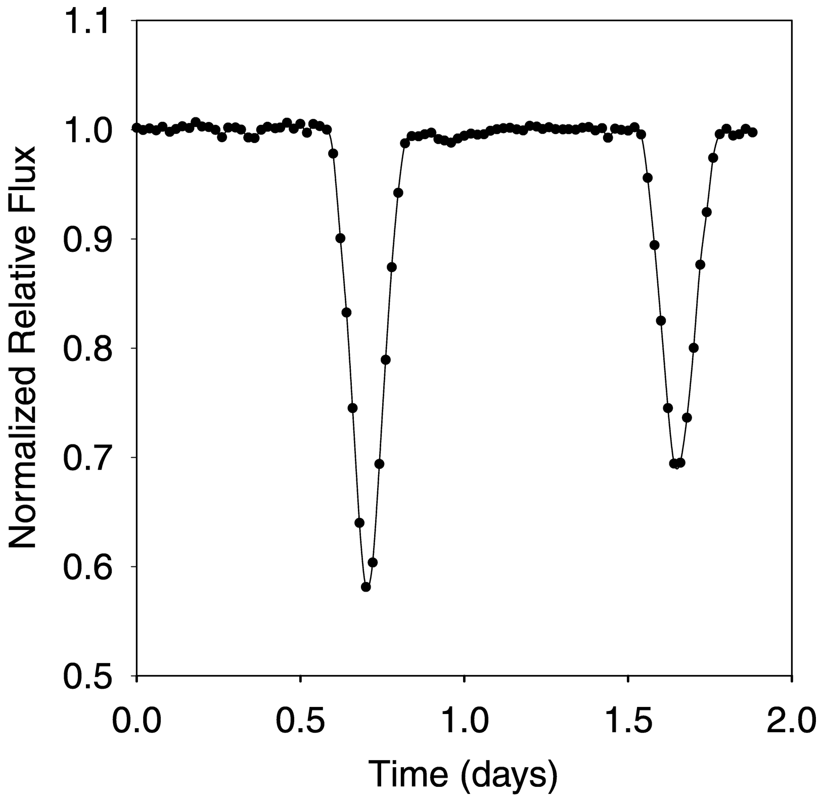
Fig. 7.— Star 805 with a period of 1.9 days and dips of 60% and 30%.
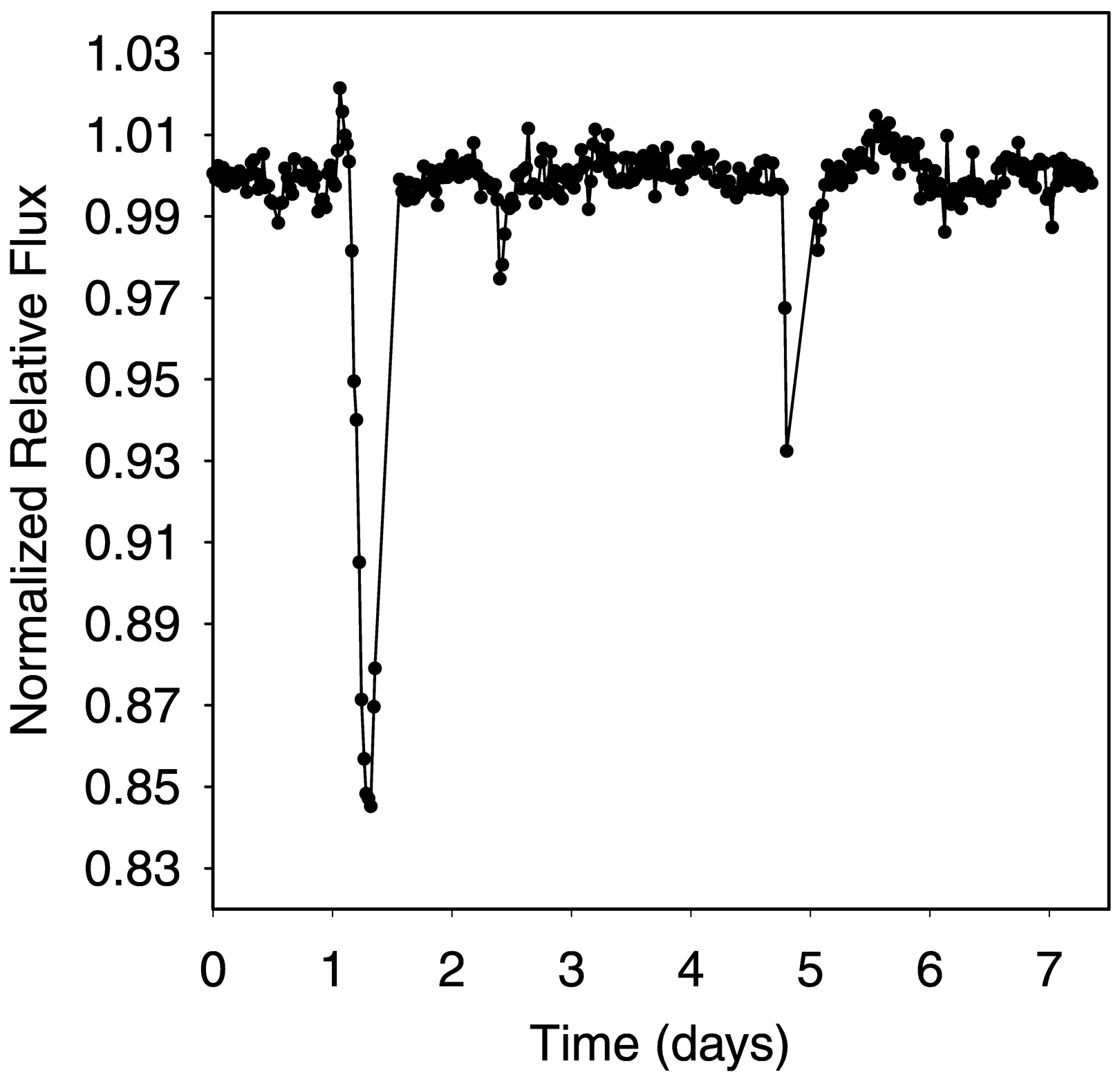
Fig. 8.— Star 1918 with a period of 7.17 days and amplitudes of 15% and 6%.
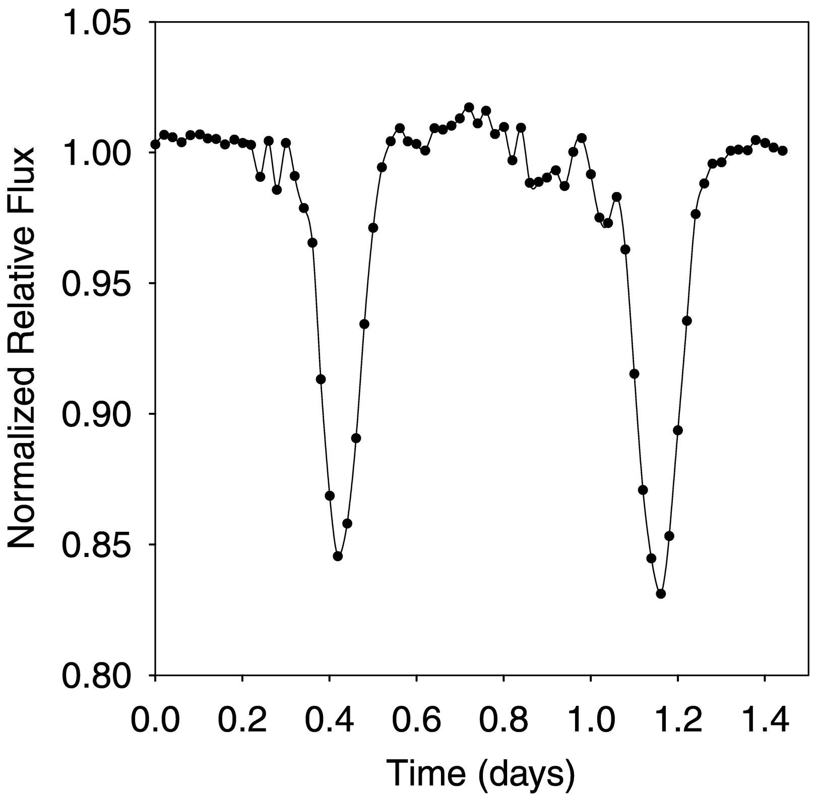
Fig. 9.— Star 874 with a period of 1.44 days and amplitudes of 16% and 17%.
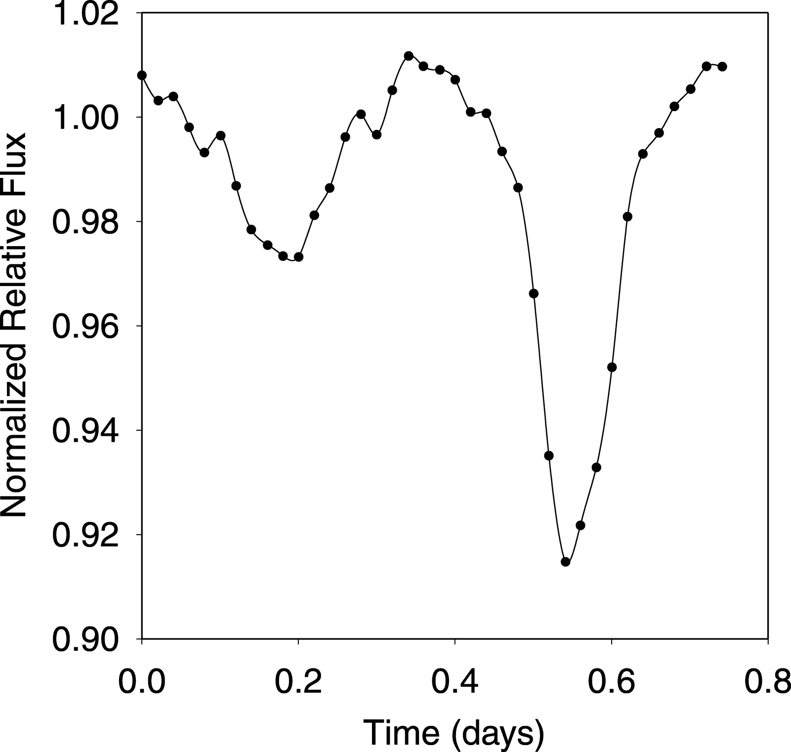
Fig. 10.— Star 3731 with a period of 0.7598 days and amplitudes of 9% and 3%.
Several stars showed low‐amplitude transits as, for example, in Figures 11 and 12. The data for these two stars have been folded and binned into 30 minute periods. The mean deviation for the binned points is about 0.1% when several data strings are folded for the purpose of discovering low‐amplitude transits. Hence, transit amplitudes of 1%–2% from Jovian‐size planets can be readily detected. However when high‐resolution spectra were obtained for both of these stars, they were found to be double‐lined binaries so similar in size as to have indistinguishable transit depths. (Note that this fact implies that the photometric periods shown in the figures must be doubled.) The low amplitude of the transits is explained if the stellar orbital planes are tipped from the line of sight by approximately 9° and 14° (for stars 1433 and 937, respectively), causing both binaries to exhibit grazing transits. Figure 13 shows the spectral region near the Hβ line for star 937. Two absorption lines due to the Doppler‐shifted Hβ line are apparent.
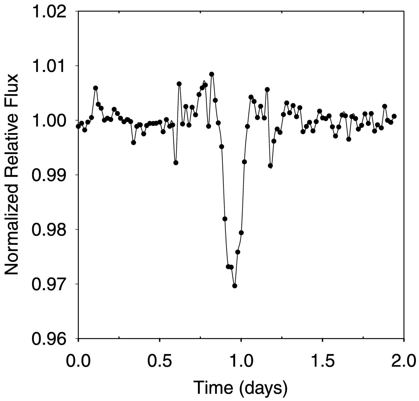
Fig. 11.— Folded and phased light curve for star 1433. Note that the actual period is twice what is shown here.
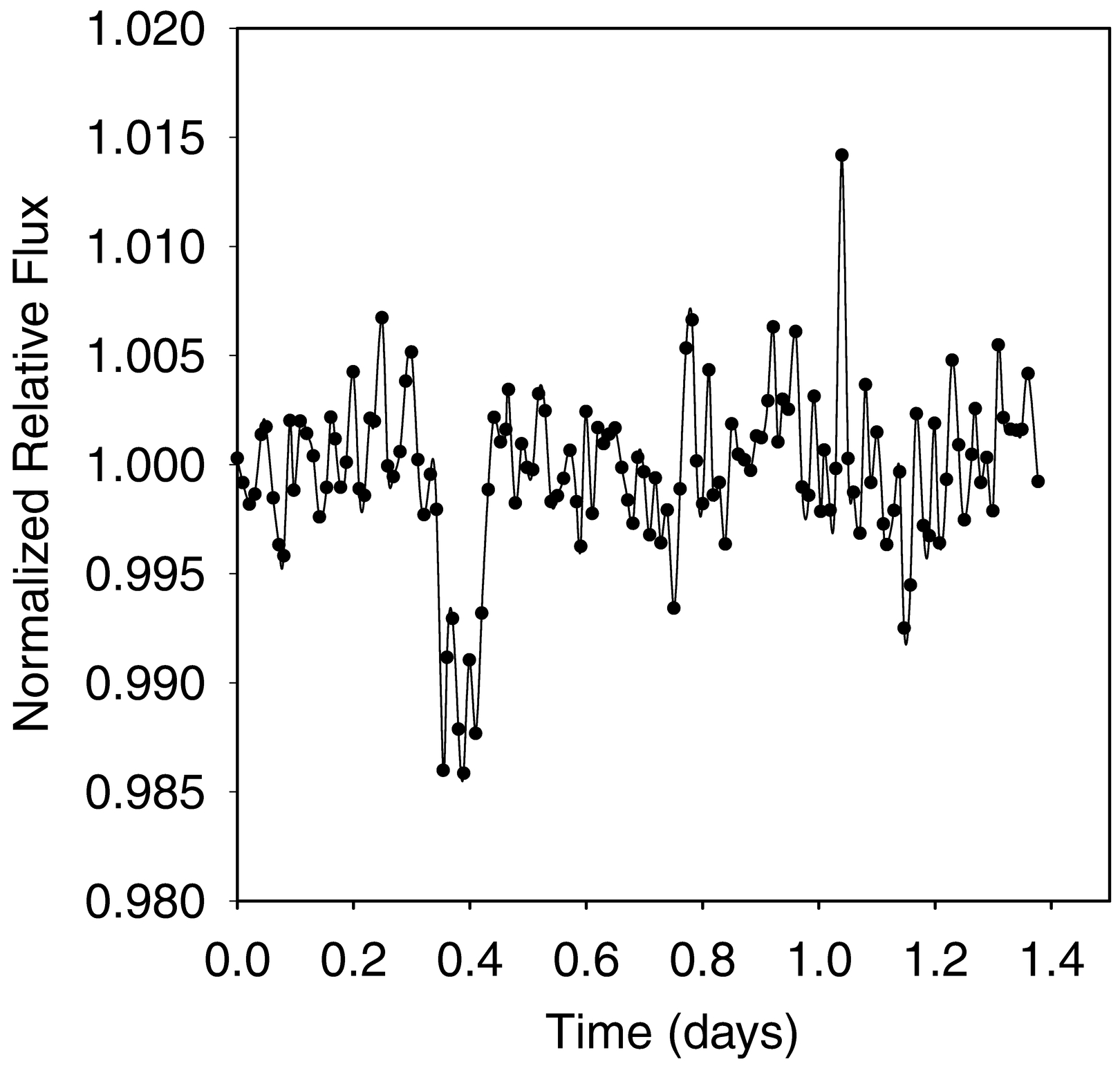
Fig. 12.— Folded and phased light curve for star 937. Note the absence of a second dip and the very low amplitude of the transit (1.3%). Note that the actual period is twice what is shown here.
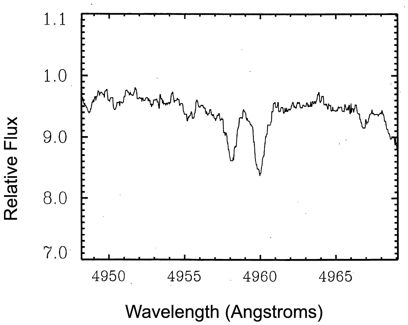
Fig. 13.— Spectra near Hβ line of star 937. (G. Marcy, P. Butler, & J. Lissauer 1999, personal communication).
Figure 14 is the folded and phased light curve for star 3047. The transit depth is 3% with a period of 4.65 days. Radial velocity measurements by D. Latham (1999, personal communication) are presented in Figure 15. The Doppler velocity data indicate that the period is exactly the photometric period. The combined data were used to obtain a preliminary solution for the structure of the system. It showed the system to be a single‐lined, high mass ratio (4:1) binary with a primary of late‐F spectral type and a secondary consistent with a mid‐M spectral type dwarf.
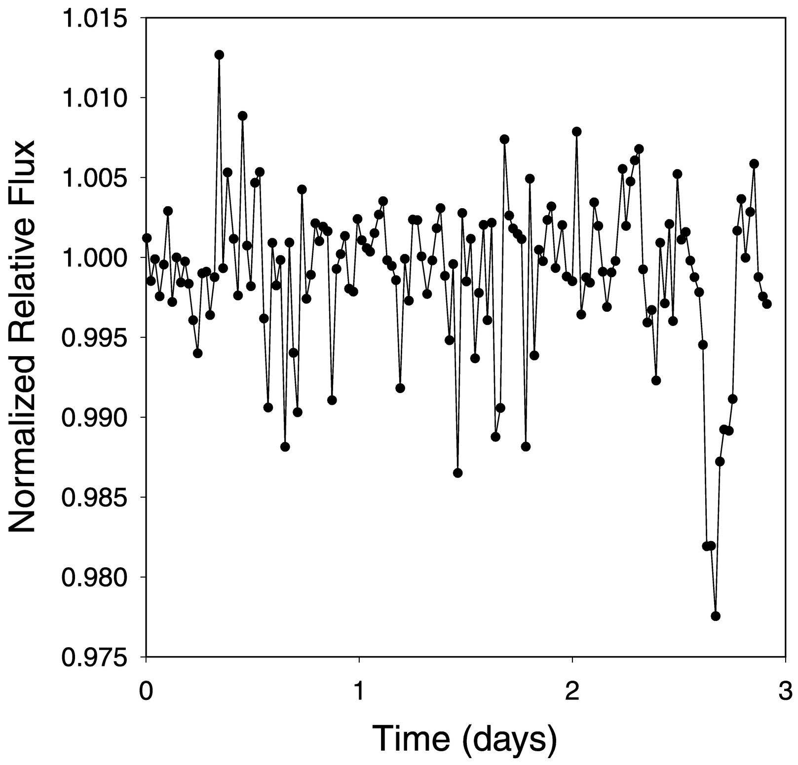
Fig. 14.— Folded and phased light curve for star 3047
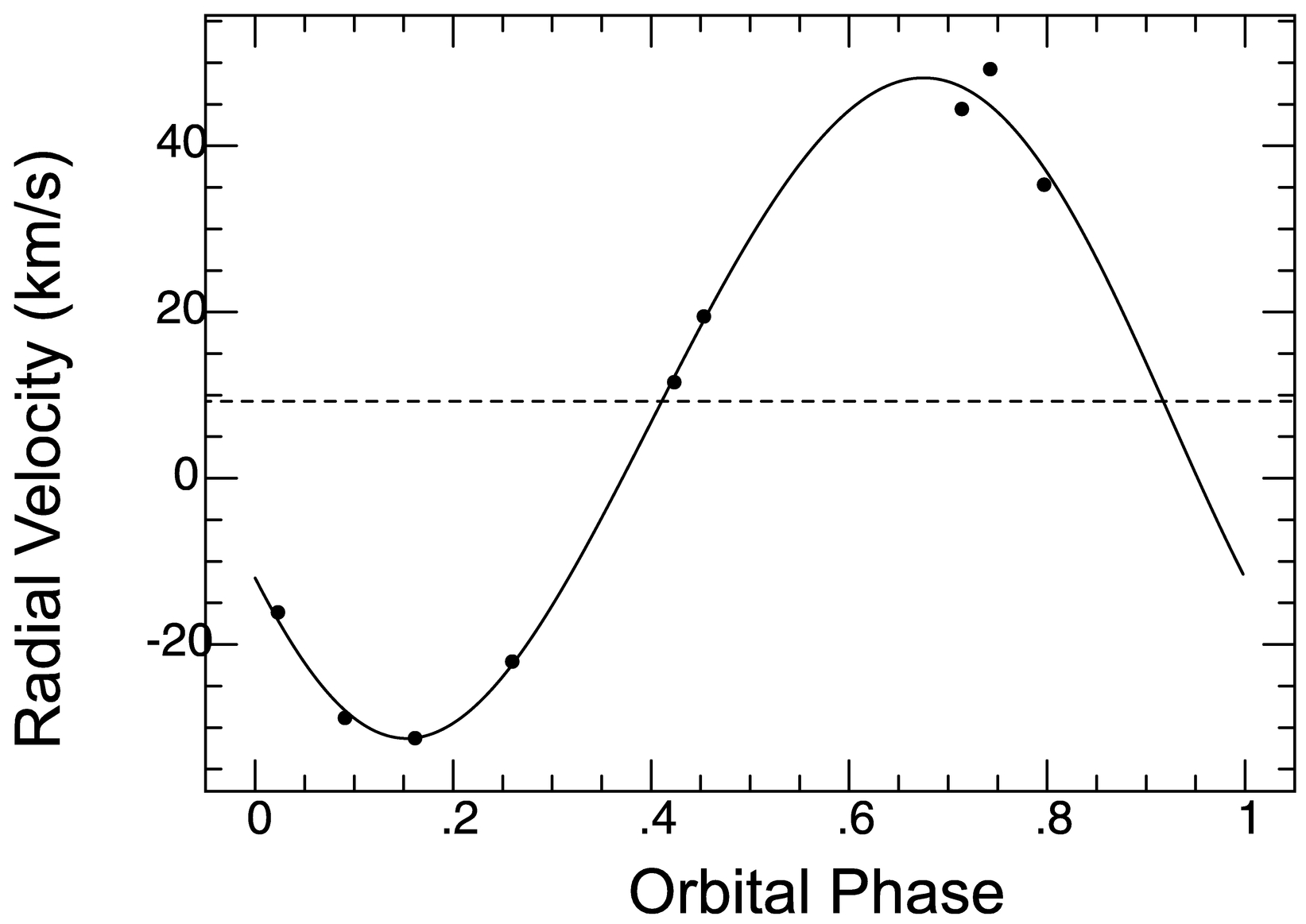
Fig. 15.— Doppler velocity measurements (D. Latham et al. 1999, personal communication) for star 3047.
In early November of 1999, two groups announced the discovery of a planet orbiting HD 209458 in the Pegasus constellation (Charbonneau et al. 2000; Henry et al. 2000). At this time of the year, the predicted transits occur about the time the star sets as seen from Lick Observatory. Because the transit occurred about the time that the star set, the observations were necessarily made at unusually high air mass. The symbols shown in Figure 16 shows the extinction‐corrected, normalized light curve we obtained for HD 209458 on that date. The solid line represents the predictions based on the work of Charbonneau et al. (2000) and Castellano et al. (2000). Both the limb crossing time (25 minutes) and the measured amplitude of the transit (1.6%) are consistent with those found by Charbonneau et al. Our best fit to the time of onset of the transit is based upon the transit epoch from Charbonneau et al. (2000) but uses the orbital period derived from the Hipparcos observations of HD 209458 by Castellano et al. (2000).
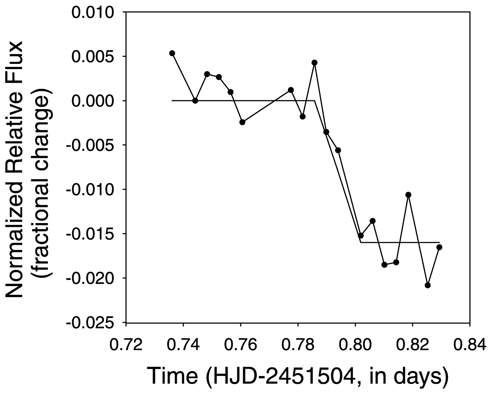
Fig. 16.— Comparison of the measured and predicted flux for the 1999 November 22 transit of a planet orbiting HD 209458.
Ordinarily, photometry is done as close to the meridian as possible to mitigate the error introduced by scintillation and rapid extinction variations that are associated with high air mass. For this reason, measurements are usually made at an air mass less than 1.5 and seldom made at an air mass as large as 2.0. Because the November 22 event was the last opportunity to observe the transit, observations were made even though the air mass ranged from 1.5 to 4 during the measurements. Figure 17 shows the measured rapid increase in standard deviation of the fluxes of the seven comparison stars at the time of the measurements. The solid curve shows the expected level of scintillation noise (Young 1974). The agreement between the measurements and the predictions demonstrates that the system was operating at a precision limited only by properties of the atmosphere. The observations were terminated at an air mass of 4 because the S/N had dropped below 2.5 at that point.
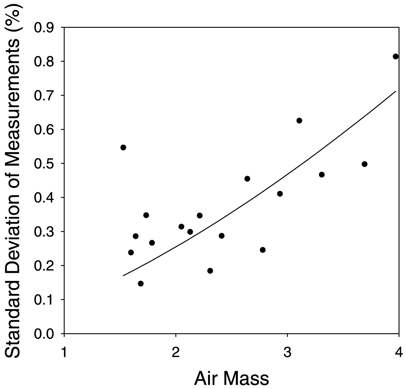
Fig. 17.— Comparison of the standard deviation of the fluxes of the comparison stars with the prediction of scintillation noise by Young (1974).
A comparison of the light curves of the comparison and target stars is shown in Figure 18. The dashed curves represent the time variation of flux from the seven comparison stars, whereas the solid curve shows the variation from the target star HD 209458. It is clear that although the scatter of the measurements grows rapidly with time, the time variation of the target star is distinctly different from those of the comparison stars. These observations are in excellent agreement with the predictions of Charbonneau et al. (2000).
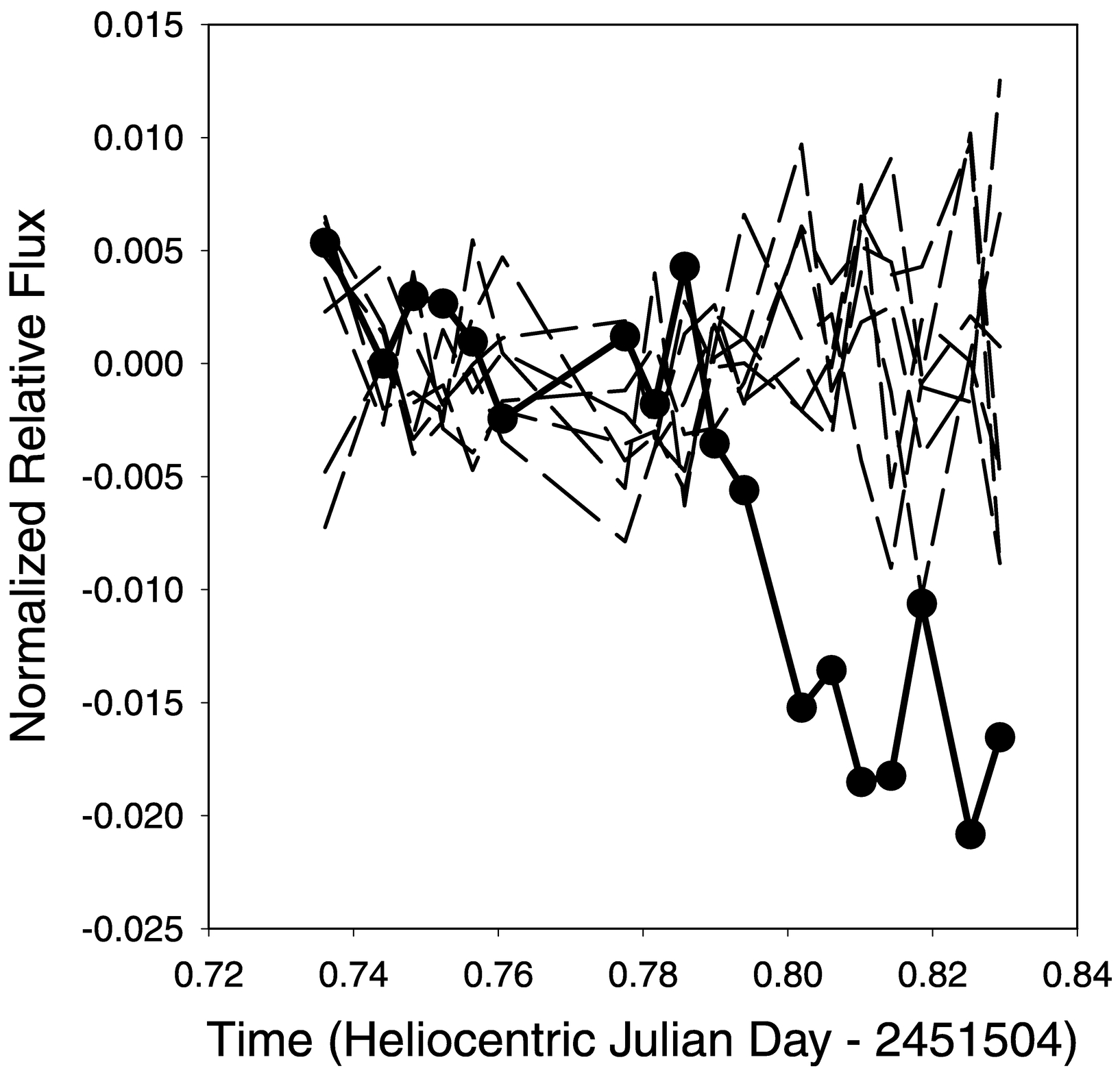
Fig. 18.— Measured fluxes of comparison stars and HD 209458 vs. time. (Dotted lines represent the comparison stars, and the solid line represents the time variation of HD 209458.)
9. CONCLUSIONS
A small photometer to detect extrasolar planets has been constructed and tested. It simultaneously monitors 6000 stars in star fields in the Galactic plane. A method of differential relative photometry is used to maximize the precision of hour‐to‐hour samples. When the data are folded to discover low‐amplitude transits, stars showing repeated transits with depths of 1% or more are readily detected. This precision is sufficient to find Jovian‐size planets orbiting solar‐like stars, which have signal amplitudes from 1% to 2% depending on the inflation of the planet and the size of the star.
Complex data processing of the images is necessary to compensate for the motions of the images due to imperfect polar alignment and differential refraction. A polynomial coordinate transformation of each image is required to correct the nonlinear scale changes and rotation that occur during the night. The numerical overhead for the PSF fitting is greatly reduced by first solving for the motions of a subset of stars and then interpolating the motions across the field. This method provides an efficient, single‐parameter, linear least squares approach to determining the flux of each star in each image. For the most well‐behaved stars, the 7 minute, image‐to‐image relative precision is about 3 × 10⁻³ before any period folding is done to reduce the noise. After data folding is done, the hour‐to‐hour precision sometimes reaches 1 × 10⁻³.
An investigation of possible noise sources indicates that star field crowding, scintillation noise, and photon shot noise are not the major noise sources for stars brighter than a visual magnitude of 11.6. An investigation is underway to determine if image motion over the CCD detector is the major noise source.
Nearly 50 eclipsing binary stars have been found in the first star field of 6000 stars, many with transit amplitudes of only a few percent. Spectroscopic measurements were made on three stars that showed only one transit per period. Two of these were found to be nearly identical stars in binary pairs orbiting at double the apparent photometric period. One was found to be a high mass ratio single‐lined binary orbiting with the observed photometric period. The 1999 November 22 transit of a planet orbiting HD 209458 was clearly observed at the predicted time and amplitude. These results demonstrate that the Vulcan photometer and the associated data reduction and analysis techniques have the precision necessary to detect Jovian‐size planets orbiting solar‐like stars.
The authors would like to thank the observers who spent many sleepless nights obtaining the data, especially Tim Castellano, Tony Dobrovolskis, Wendy Hansen, Carol Harper, Lynn Harper, Ralph Libby, Alan Meyer, Patrick Maloney, and William Trublood. The superb work of the machine shop headed by Dave Scimeca was critical to the success of the project. Scripts to control and automate the operation of the camera were written by Bob Slawson of the Rochester Institute of Technology. John Caldwell, on sabbatical from York University, investigated the influence of star crowding on photometric precision. Robert Yee directed system operation and maintenance. Kim Kubota (Orbital Science Corporation) and Walt Miller (Man Tech Corporation) directed the observers. The cooperation and help of the Lick Observatory staff, especially Remington Stone, and their permission to use the Crocker Dome made the project possible. Special thanks are due to Geoff Marcy, Paul Butler, Jack Lissauer, Eduardo Martin, David Ardilla, and Dave Latham, who made spectroscopic observations of candidate stars. Advice from Tim Brown (HAO, UCAR), Ted Dunham (Lowell Observatory), and Laurence Doyle (SETI Institute) contributed the success of the project. The patience, support, and funding received from Origins and Advanced Project Offices at NASA Headquarters and the Astrobiology Office at NASA Ames are gratefully acknowledged.
Footnotes
- 2
We distinguish between accuracy and precision as follows; accuracy is measurement to an absolute standard, whereas precision is the repeatability of the measurement without regard to whether the value is accurate.