
ABSTRACT
Stellar intensity scintillation in the optical was extensively studied at the astronomical observatory on La Palma (Canary Islands). Atmospheric turbulence causes "flying shadows" on the ground, and intensity fluctuations occur both because this pattern is carried by winds and is intrinsically changing. Temporal statistics and time changes were treated in Paper I, and the dependence on optical wavelength in Paper II. This paper discusses the structure of these flying shadows and analyzes the scintillation signals recorded in telescopes of different size and with different (secondary‐mirror) obscurations. Using scintillation theory, a sequence of power spectra measured for smaller apertures is extrapolated up to very large (8 m) telescopes. Apodized apertures (with a gradual transmission falloff near the edges) are experimentally tested and modeled for suppressing the most rapid scintillation components. Double apertures determine the speed and direction of the flying shadows. Challenging photometry tasks (e.g., stellar microvariability) require methods for decreasing the scintillation "noise." The true source intensity I(λ) may be segregated from the scintillation component ΔI(t,λ,x,y) in postdetection computation, using physical modeling of the temporal, chromatic, and spatial properties of scintillation, rather than treating it as mere "noise." Such a scheme ideally requires multicolor high‐speed (≲10 ms) photometry on the flying shadows over the spatially resolved (≲10 cm) telescope entrance pupil. Adaptive correction in real time of the two‐dimensional intensity excursions across the telescope pupil also appears feasible, but would probably not offer photometric precision. However, such "second‐order" adaptive optics, correcting not only the wavefront phase but also scintillation effects, is required for other critical tasks such as the direct imaging of extrasolar planets with large ground‐based telescopes.
Export citation and abstract BibTeX RIS
1. INTRODUCTION
Extensive studies of stellar intensity scintillation (arising in the terrestrial atmosphere) have been made at the observatory on La Palma (Canary Islands). Three papers present the results. Paper I, on statistical distributions and temporal properties (Dravins et al. 1997a), analyzed the temporal statistics of scintillation and its behavior on timescales from microseconds to seasons of year. That first paper also described the general experimental arrangements and gave an overview of scintillation mechanisms and phenomena in general. Paper II, on dependence on optical wavelength (Dravins et al. 1997b), dealt with the more subtle differences between different optical colors in scintillation amplitudes, timescales, and delays. Finally, the present paper, Paper III, on effects for different telescope apertures, evaluates how scintillation appears when observed through telescope pupils with varying diameter, shape, and central obscuration. It concludes by discussing the inverse problem, i.e., how to choose telescope optics and how to perform observations and data analysis, in order to minimize undesired effects of scintillation "noise."
Atmospheric turbulence causes "flying shadows" on the ground, and intensity fluctuations occur because this pattern not only is carried by the winds but also is intrinsically changing. The origin of this structure (which in essence is the atmospheric speckle pattern) was discussed in Paper I. Here we will evaluate observations and theory of these "flying shadows," and analyze what scintillation is perceived by different telescopes, integrating this shadow pattern over their respective entrance pupils. Measurements in sequences of smaller apertures will be extrapolated and modeled to embrace also very large telescopes in the 8 m class. It will be illustrated how, for a given telescope diameter, scintillation may differ significantly, depending on the central (secondary‐mirror) obscuration, or its inverse, i.e., the degree of apodization. Elongated or double apertures permit a direct determination of the speed and direction of these flying shadows.
One main purpose of this project is to better understand actual (nonideal) scintillation properties at premier observatory sites such as La Palma. An envisioned application is to exploit this improved understanding to search for photometric variability of very low amplitude (perhaps that expected from stellar oscillations or from exoplanet transits), or for very rapid fluctuations in astronomical objects, such as those arising from instabilities in mass flows around compact objects. A successful segregation of the probably quite subtle astrophysical variability from the superposed atmospheric fluctuations may require a detailed correction for the atmospheric effects.
How is the observing strategy to be optimized? Different telescope apertures emphasize certain spatial, and consequently temporal, parts of the scintillation. A large collecting area decreases the scintillation power by filtering out small‐scale fluctuations, while aperture edges that are apodized in intensity transmission depress in particular the most rapid scintillation components. Thus, an optimization of the telescope entrance pupil may enhance the detective sensitivity for specific types of astrophysical variability. Further, what is the trade‐off between using a large telescope for a shorter time versus one or several smaller telescope(s) for a longer time?
Optimum methods for the most precise ground‐based stellar photometry are yet to be developed and verified, both for single large telescopes and for arrays of smaller ones. Promising passive systems involve time‐resolved measurements over the spatially resolved telescopic entrance pupil area, simultaneously in several photometric colors. The signal of astrophysical variability would then be segregated from the atmospheric one through modeling the latter in terms of its temporal, spatial, and chromatic dependences. Adaptive systems can also be envisioned, correcting not only the atmospherically distorted phase but also the amplitude, reducing or even eliminating scintillation effects for imaging applications. Such real‐time systems (working together with "ordinary" phase‐correcting adaptive optics) appear required for some very challenging direct‐imaging tasks, such as that of exoplanets.
This paper is organized as follows: § 2 discusses the "flying‐shadow" properties, including their aperture "filtering." Section 3 exploits power spectra measured on La Palma to predict scintillation in very large telescopes. Section 4 examines scintillation signatures measured in telescopes with circularly symmetric but sharp apertures, § 5 in symmetric but apodized ones, and § 6 in double apertures and those of elongated shape. Finally, § 7 concludes this whole series of papers with schemes for optimally circumventing scintillation "noise" in astronomical observations.
2. THE STRUCTURE OF "FLYING SHADOWS"
2.1. Previous Studies of Atmospheric Shadow Patterns
We will now evaluate how atmospheric scintillation is perceived in telescopes of different apertures, i.e., integrating different parts of the flying‐shadow patterns over the pupil plane of each telescope. We begin by reviewing some previous observations of such flying shadows.
2.1.1. Stellar Observations
The early literature contains a number of photographs, showing flying shadows on telescope mirrors (Gaviola 1949; Mikesell, Hoag, & Hall 1951; Protheroe 1955a). However, these images convey a false impression of the shadow pattern being elongated into "bands," an effect that was caused by the longish exposure times required, during which the imaged pattern was stretched out along the direction of the prevailing winds. During a typical exposure of 25 ms, with a typical wind speed of 20 m s−1, the pattern is displaced by half a meter, a distance much greater than characteristic shadow scales (given by the Fresnel‐zone size rF = √λh, on the order of 5–10 cm; Paper I). To freeze the pattern requires exposure times of no more than a few milliseconds, not feasible with the then available photographic emulsions. Nevertheless, these early records showed that the turbulence layers causing the shadow patterns were multiple and unstable, and that the fine structure in the patterns could change very rapidly, in mere fractions of a second.
More quantitative studies followed, using photomultiplier detectors and various double and multiple entrance apertures. Thus, Keller (1955), Protheroe (1955b), Barnhart, Protheroe, & Galli (1956), Keller et al. (1956), and Protheroe (1961, 1964) deduced spacetime autocorrelation functions and other statistical properties of the shadow structure.
Modern studies, analyzing the two‐dimensional spatiotemporal power spectra of shadow patterns, clearly reveal the multilayer structure of winds and turbulence structures in the upper atmosphere (Vernin & Roddier 1973; Vernin & Azouit 1983; Caccia, Azouit, & Vernin 1987; de Vos 1993). Images of the telescope pupil, recorded in very short exposure times of a few milliseconds, no longer show any evidence for the "banded" appearance of early photographic recordings; the frozen shadow pattern cast by a star now appears isotropic, as theoretically expected.
2.1.2. Solar‐Eclipse Shadows
During some tens of seconds before and after solar‐eclipse totality, when the almost‐eclipsed Sun constitutes a source of very small angular width, the flying‐shadow pattern can be perceived also with the unaided eye (although the intensity fluctuations amount to only a few percent). For introductory reviews, see Marschall (1984) and Codona (1991). Over long horizontal light paths, analogous phenomena may be seen projecting onto vertical walls, in the light cast by the low Sun when it is almost occulted by sharp features on the horizon, in the light cast by Venus, or from powerful artificial‐light beams.
Such flying shadows were noted by visual observers a long time ago. However, their transient nature made photographic recordings very difficult, and the paucity of precise observations led to a proliferation of exotic theories for their origin. More quantitative photoelectric measurements from recent decades (Young 1970b; Hults et al. 1971; Quann & Daly 1972; Klement 1974; Marschall, Mahon, & Henry 1984; Jones & Jones 1994) demonstrated how the shadow bands become narrower and more closely spaced as totality approaches and how their power spectra are quite similar to those for stellar scintillation.
The scintillation theory of eclipse shadows was very well presented by Codona (1986). The primary difference to the stellar case is that the illumination source is not pointlike but rather crescent‐shaped. While shadow patterns from stars are statistically isotropic, solar shadow bands are not, because of the anisotropic brightness distribution of the uneclipsed solar crescent.
Further differences exist because of the varying spatial extent of the solar crescent. For times greater than about 20 s before (or after) totality, the solar shadows are dominated by turbulence near the ground. Turbulence at the tropopause (important in the stellar case) has almost no impact on shadow bands until 2–3 s from totality, when the uneclipsed solar portions start to become pointlike. Only during these short time intervals does a wavelength dependence develop (cf. Paper II). Shadow bands are related to the same turbulence responsible for seeing; good seeing is predicted to cause a poorer shadow‐band contrast.
2.2. Observed Aperture‐Size Dependences
Among the dependences on spatial sampling of the flying‐shadow pattern, perhaps the most obvious is the dependence of scintillation amplitude on telescope size. That the intensity variance decreases with increasing telescope collecting area had been realized already in early measurements (see, e.g., Mikesell et al. 1951; Ellison & Seddon 1952; Siedentopf & Elsässer 1954; Bufton & Genatt 1971; Iyer & Bufton 1977; Dainty et al. 1982; Stecklum 1985).
Another distinct signature of aperture averaging is the shifting of the relative frequency content in the power spectrum toward lower frequencies (the spatially smallest and temporally fastest fluctuations are preferentially averaged out, making scintillation slower), as studied by Mikesell et al. (1951), Mikesell (1955), Protheroe (1955a), Darchiya (1966), Young (1967), Gladyshev et al. (1987), and others.
The precise dependence of terrestrial and laboratory scintillation on the size of the sampling (or transmitting) aperture may be used to segregate competing theories, especially in cases including nonlinear scintillation effects. Such dependences are also used to remotely sense properties of turbulent media. Quite a number of experiments have been made, some of which may be relevant also for astronomical applications: Kerr & Dunphy (1973), Titterton (1973), Homstad et al. (1974), Yura & McKinley (1983), and Arsen'yan & Zandanova (1987).
2.3. Theory of Aperture "Filtering"
Scintillation depends not only on the size of the aperture, but also on its geometrical shape (circular, annular, elongated, double), possible pupil areas of reduced transmission (central stop, spider vanes, apodization), and (for radially nonsymmetric apertures) its angular orientation relative to the motion of the flying shadows. Such dependences, on one hand, increase the complexity of analysis but, on the other hand, permit one to disentangle various scintillation properties and guide us toward schemes of reducing undesired scintillation. Further complications (and possibilities) enter for very strong (saturated) scintillation; if the aperture sizes approach either the inner or outer scales of turbulence; and for nonideal statistics of the atmospheric refractive‐index fluctuations.
As already noted in §§ 4.1 and 5.1 of Paper I, incorrect arguments were used in the past, involving the false assumption that patches in the flying‐shadow pattern would be statistically independent. However, wavefront irregularities merely redistribute the starlight, and the bright and dark parts of the shadow pattern are not independent. One area can be brighter than average only by gaining irradiance from neighboring regions, which are then necessarily darker than average. This redistribution is accurately portrayed by Fourier analyzing the brightness distribution; each sinusoidal spatial‐frequency component has its brighter parts exactly balanced by adjoining darker ones.
In an astronomical context, theoretical studies of the change of scintillation spectra with telescope aperture size and shape have been done by Tatarski (1961), Reiger (1963), and Young (1967, 1969), and reviewed by Roddier (1981).
In the context of laser‐beam propagation, modeling of aperture‐averaging effects has been done by Fried (1967), Wang, Baykal, & Plonus (1983; Gaussian weighting function for the receiver aperture, coherent beams), Mazar & Bronshtein (1990; numerical solutions for plane and spherical waves), Churnside (1991; approximate expressions, large apertures, weak and strong turbulence, different inner scales), Andrews (1992; exact expressions for weak turbulence, plane and spherical waves), and Bass et al. (1995; analytic expressions, plane and spherical waves, weak fluctuations; refractive index fluctuations with inner scale); a review is given in Sasiela (1994). For specific effects of aperture‐shape dependence, see Belov & Orlov (1978, 1980; circular and annular) and Cho & Petersen (1989; optimal choice for given scintillation statistics).
2.3.1. Computing Aperture Effects
For the next several chapters, we will calculate synthetic power spectra and autocovariance functions to compare with our observations. The purpose is not to model the precise atmospheric conditions above La Palma but rather to obtain scintillation functions from a model that is sufficiently simple for the comprehension and traceability of effects, yet capable of identifying subtle differences between different types of aperture, and of allowing an extrapolation of scintillation properties to much larger telescopes.
Simple effects from aperture averaging were discussed in Paper I, e.g., a geometric‐optics approximation predicts the intensity variance σ2I in the focal plane to obey
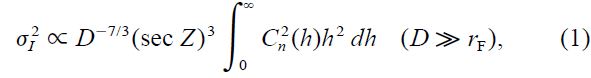
where C2n(h) is the refractive index structure coefficient, h is altitude in the atmosphere, and Z is the zenith distance. This approximation (neglecting wavelength‐dependent diffraction) is valid for circular aperture diameters D (much) greater than the Fresnel‐zone size rF = √λh (in the zenith; otherwise √λhsec Z). Then the amount of scintillation is independent of wavelength and merely decreases with increasing D.
2.3.2. Aperture Filtering of Power Spectra
Our modeling follows Young (1969, 1970a); see also Roddier (1981). The Kolmogorov spectrum of (three‐dimensional) isotropic turbulence throughout the atmosphere is used to compute the spatial intensity spectrum of the (two‐dimensional) flying‐shadow pattern falling onto the ground. Approximate allowances are made for diffraction, atmospheric dispersion, and seeing, integrated through an (assumed) exponential atmosphere with a certain turbulence scale height. The spatial‐filter function of the telescope aperture is multiplied by the two‐dimensional power spectrum of the shadow pattern, and the product is numerically integrated in both spatial‐frequency dimensions to give the total modulation power.
We assume a single wind speed (in the x‐direction) and consider a monochromatic optical wavelength of 500 nm. Further, following Taylor's hypothesis, the temporal variation of the illumination pattern is given by a linear shift at constant velocity equal to the wind speed. The modeling does not provide normalizing factors for either the strength of the turbulence or for the calibration of the temporal frequency scale (which depends on the actual wind speed). Both these parameters are obtained by fitting the synthetic functions to actual data, as recorded during representative summer conditions on La Palma.
Through appropriate integrations, one may obtain different statistical descriptions of the shadow pattern (autocorrelation, power spectrum, structure function). For example, by integrating the spatial power spectrum over the spatial‐frequency coordinate perpendicular to the wind direction, and using the projected wind speed to transform the spatial frequency into temporal frequency, we obtain the temporal power spectrum of scintillation, P(f).
Consider a circular telescope aperture of radius a. Its response to modulation at spatial frequency k is found by integrating the sinusoidal intensity fluctuation over the aperture (k = 2π/d, where d is a spatial period in the shadow pattern; cf. § 4.3 in Paper I). The result is that the detected modulation power is diminished by the factor
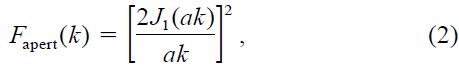
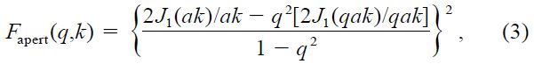
which is called the aperture filter function (Young 1969; Roddier 1981). J1 is the Bessel function, familiar from diffraction theory. Equation (2) has the same form as the diffraction pattern of a circular aperture, and the filter function for any aperture indeed has the form of its diffraction pattern, normalized to unity at k = 0. For example, an annular aperture of outer radius a and inner radius qa has the filter function (Young 1967)
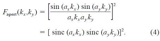
and for a rectangular aperture of width 2ax in the x‐direction and 2ay in the y‐direction, one has (Young 1969)
Similarly, filter functions for apodized apertures are calculated. Apodizing a zone of width w at the edge of a circular aperture gives an amplitude transmission function that can be approximated by the convolution of a circular aperture of radius (a - w/2) (where a is the clear‐aperture radius) with a small circular aperture of diameter w/2 (radius w/4). This operation makes the amplitude‐transmittance function very nearly (but not exactly) sinusoidal. Convolution in the spatial domain corresponds to multiplication of the corresponding functions in the spatial‐frequency domain, and the spatial‐filter function of such an apodized aperture is
If w/4≪(a - w/2), the second factor is nearly unity, and apodizing a narrow outer zone has practically the same effect as reducing the clear aperture by half the width of the zone. We may regard aeff = a - w/2 as the effective radius of the apodized aperture. The benefits of apodizing do not appear until the second factor in equation (5) begins to decrease appreciably.
More complex apertures, e.g., annular ones with inner and outer apodized edges, are computed by suitably combining various clear and apodized portions.
Once the aperture filter function Fapert(k ) is known,k = (kx,ky), its effect is obtained by multiplying the (two‐dimensional) shadow‐pattern power spectrum P2(k ) by Fapert(k ):
Thus, the frequency spectrum, autocorrelation function, and other descriptors are obtained by using P*2(k ), the filtered spectrum of the smeared shadow pattern, instead of P2(k) itself.
2.3.3. Functional Trends and Approximations
We now examine the main trends of the functions. Some apparent complexity comes from the oscillations in the aperture‐filter functions, in particular the "beats" between the oscillations of the Bessel functions in obscured apertures. These originate from the idealized model assumptions, and we shall neglect these details, concentrating on the general trends.
The three‐dimensional isotropy of the assumed Kolmogorov turbulence causes a two‐dimensionally isotropic shadow pattern with power spectrum P2(k ). If the telescope aperture has circular symmetry,Fapert(k ) is also isotropic. This makes P*2(k ) in equation (6) isotropic as well. At low frequencies, where all the filter functions are nearly unity,P*2 is proportional to k1/3. Eventually, k becomes large enough to make any filter function begin to decrease rapidly. Since all our filter functions have (oscillating) tails whose envelopes fall off as some substantial power of k, this decrease effectively truncates the integration.
For example, the aperture filter for a radially symmetric aperture with sharp edges falls off (apart from the oscillations) as k-3 (eqs. [2] and [3]). This applies to apertures much larger than the Fresnel‐zone size; for smaller ones, diffraction effects cause a more rapid cutoff as k-4 (Young 1969, 1970a). The filter for an apodized aperture has two Bessel‐function factors. It falls as k-3 when the main factor (associated with the outer radius aeff) begins to decrease rapidly, and as k-6 when the second factor (associated with the apodizing‐zone width w) becomes effective. In every case, the falloff begins where the argument of a filter is of order unity. The rectangular aperture (eq. [4]) has asymmetric properties; its filter drops as k-2 along the x or y edges, but as k-4 along its diagonal.
The total modulation power, i.e., the intensity variance σ2I, is found by integrating P2 up to the point where the first filter truncates the integration. As the lowest turnover frequency corresponds to the largest spatial dimension, this is usually set by the telescope aperture. The aperture filter function turns down when ak ≈ 1, or k ≈ 1/a. The integral is thus
if we use the isotropy to write d k as k dk dø. The 2π comes from integrating over ø.
To obtain results for the time domain, we must write d k as dkxdky and integrate over dky. At low frequencies, P2 is proportional to k1/3, and the integration extends from ky = 0 to ky ≈ 1/a. Then
if we use the fact that ky ≈ k in the region where the integrand is large. We could also have obtained this result by noting that the total intensity variance σ2I is spread over the region from kx = 0 to kx ≈ 1/a, so that the low‐frequency power must be proportional to σ2I/(1/a)∝ a-7/3/a-1 = a-4/3.
At high frequencies, the integrand falls off as k1/3 times the tail of the filter function, which is a large negative power of k. Thus, the function P*2(k) looks somewhat like a circular crater, with its lip at the value of k where the filter turns down. The outer slopes, apart from the oscillations, fall off as k-3 + 1/3 = k-8/3 for large sharp‐edged apertures,k-4 + 1/3 = k-11/3 for small ones, and as k-17/3 for our apodized apertures. The region where the integrand is appreciable extends for a distance in ky comparable to kx. Thus, the tail of the one‐dimensional power spectrum is
where p = 3 for sharp‐edged ones, 4 for apertures smaller than the Fresnel‐zone scale, and 6 for apodized ones. Thus, the tails fall off as k-5/3,k-8/3, and k-14/3, respectively, in these three cases.
The turnover for a given aperture begins near kx = 1/a, or temporal frequency f = V⊥/2πa, where V⊥ is the projected wind speed. For 30 m s−1, that corresponds to about 10 Hz for a 1 m aperture. Diffraction becomes important when λhk2/4π ≈ 1, or k ≈ (4π/λh)1/2, where a typical value of h is a scale height or 8 km. For λ = 500 nm, this corresponds to about 150 Hz near the zenith. At higher frequencies, the diffraction filter reduces the tail exponent by an additional 4 units, making these tails fall off as the −17/3 power of frequency for sharp‐edged apertures and f-20/3 for apodized ones.
2.3.4. Limits to Scintillation Theory
As a final caveat for this chapter, we point out some limitations to the scintillation modeling applied here.
At the highest frequencies, there are limits in the approximations used, e.g., for the diffraction cutoff. Assuming no inner‐scale cutoff, one could just extrapolate the tails of the power laws: a slope of −5/3 up to around 100 Hz and −17/3 beyond that. However, there is evidence (§ 6.6 in Paper I) for a more rapid decrease, at shadow scales of some millimeters. This implies that very high frequency scintillation will be rather weaker than a simple power‐law extrapolation would indicate at frequencies above about 1 kHz. In this range also small structures like the supporting vanes of the secondary mirror could introduce high frequencies into the aperture filter.
The calculated scintillation spectra refer to the logarithm of the intensity, not the intensity itself. Since the scintillation amplitudes almost always are small, the practical difference should be negligible. However, as the intensity is lognormally distributed, the nonlinear transformation from logs to antilogs means that the intensity distribution will, at least in principle, contain harmonics and intermodulation (sums) of the frequencies in the log intensity spectra. These additional high frequencies could dominate the tail of the intensity spectra for small apertures, especially apodized ones.
The Kolmogorov power law is used to predict the spatial spectrum of the shadow pattern. A conclusion from Papers I and II was that the observations generally do support the validity of this Kolmogorov law for turbulence. However, the agreement is not perfect, and there could exist locations or times when atmospheric conditions might deviate. There exist alternative theories for the power spectrum of turbulence, taking a finite outer scale into account, e.g., the von Kármán spectrum (Tatarski 1961).
It would be valuable to test the predictions for very large telescopes, through actual observations. One issue that probably cannot be answered without such measurements concerns effects from the outer scale of atmospheric turbulence, i.e., the largest geometrical scales where a "turbulent" description of the atmosphere still is valid. Quite possibly, its order of magnitude is close to 10 m, the size of the currently largest optical telescopes.
3. EXTRAPOLATION TO (VERY) LARGE TELESCOPES
In this section, we will examine the behavior of scintillation power spectra in telescopes of all sizes, going from the smallest apertures (where the flying shadows are "fully" resolved) to very large telescopes (possibly approaching the outer scale of turbulence).
Although our La Palma measurements extend only to ø = 60 cm, the observed sequence of power spectra for successively larger apertures permits a rather precise fit to a theoretical sequence, extending to very large telescopes. Our model will be normalized both to the typical strength of turbulence and to the representative wind speeds observed. As a result, we will obtain representative power spectra for even (hypothetical) very large telescopes on La Palma.
3.1. Scintillation in Small Telescopes
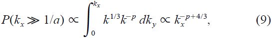
Figure 1 shows a sequence of synthetic power‐density spectra of scintillation, normalized against a sequence of observed ones. The normalization was obtained by fitting the sequence of models to representative data from La Palma, obtained during good summer conditions at 550 nm and scaled to a zenith distance Z = 45°. The best fit for the frequency scale here corresponds to a wind speed of 10 m−1 (also a typical value obtained from measurements through double apertures; § 6), while the scale for the synthetic power was adjusted vertically for best fit.
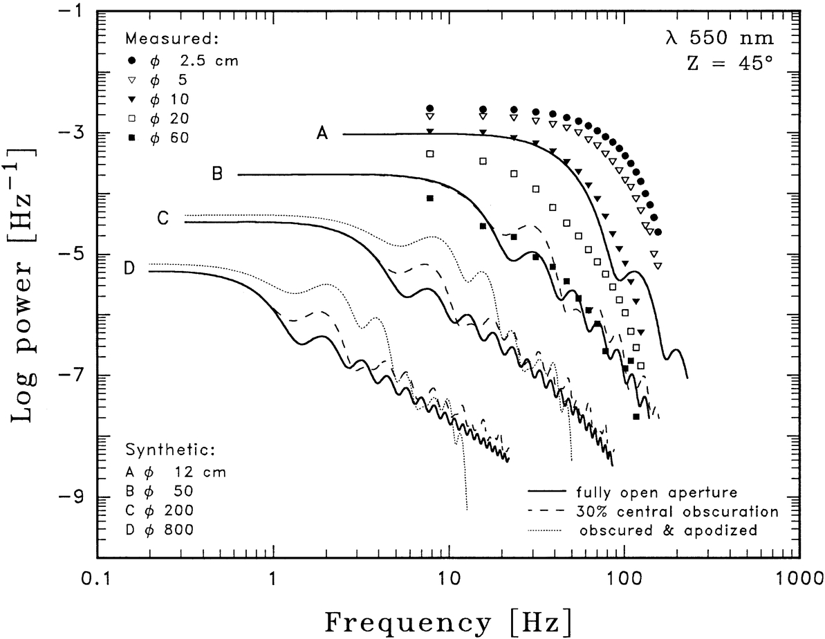
Fig. 1.— Power spectral density of scintillation in telescopes of different size. The symbols are values measured on La Palma for a sequence of small apertures. Their fit to a sequence of synthetic spectra predicts the scintillation also in very large telescopes up to 8 m diameter. Bold curves are for fully open apertures. A central obscuration (secondary mirror) increases the scintillation power, while apodization decreases it for high temporal frequencies.
Figure 1 shows P(f), the power spectral density, i.e., the amount of scintillation power per unit frequency bandwidth, as a function of frequency. The discrete symbols denote observed values, measured for small apertures of successively increasing size, from ø = 2.5 to ø = 60 cm (the same data as for 550 nm in July, in Fig. 16 of Paper I). This sequence was fitted to synthetic power spectra extending to apertures up to ø = 8 m diameter, thus predicting the scintillation also in very large telescopes. The bold curves are synthetic power spectra for fully open apertures.
The inclusion of a central obscuration, corresponding to the secondary mirror (here taken as of diameter 30% of the full one), increases the scintillation power (dashed curve), while apodization of this aperture (i.e., smoothly varying intensity transmission near the aperture edges) decreases it for high temporal frequencies (dotted curve). Effects in annular and apodized apertures are discussed in §§ 4 and 5 below.
The observed curves in Figure 1 appear like smeared versions of the models. There is no sign of any clear minima, and the data tend to fit a straighter line than the model—the "knee" is smoothed out. Such effects are expected from wind shear, and from there being different contributions from a range of heights in the atmosphere. This smearing is visible in the data for ø = 60 and 20 cm, but in smaller apertures diffraction becomes more important, and the model curves themselves become somewhat smoother; the "textbook" appearance almost always is more pronounced for the smaller apertures.
The wiggles that look like interference fringes originate in the scintillation spectrum from each atmospheric layer, because of the "sidelobes" in the telescope's diffraction pattern, and because a constant wind speed throughout the atmosphere was assumed. In reality, effects of wind shear at different atmospheric heights would wash out at least the higher order "fringes."
3.2. Calculations for Large Apertures
As seen in Figure 1, the scintillation power spectrum predicted for the largest telescopes is rather different from that in small apertures. For apertures of 8 m, there is some uncertainty whether one might reach the outer scale of turbulence (and leave the realm of validity of the model approximations). If the turbulence at such large scales should prove to be less than an extrapolation from the Kolmogorov law, scintillation power will be less.
Measurements with very large telescopes could thus be revealing about turbulence properties, although actual scintillation values cannot be expected to differ much from a Kolmogorov‐law extrapolation (obeyed by at least 4 m class telescopes; § 7.1.3 below). Assuming the outer scale to equal, e.g., 4 m, larger apertures would be equivalent to sums of independent 4 m subapertures. Very large apertures of diameter D would then depress the scintillation variance σ2I proportional to the telescope area, a steeper dependence than the Kolmogorov extrapolation for its low‐frequency component (eq. [10]).
There is a striking difference in slope of the high‐frequency tails for small and large apertures. This is caused by the smaller apertures being close to, or at, the diffraction‐limited regime, where wave‐optical (Fresnel) filtering helps cut the tail off. The large apertures just show the effects of geometric optics.
Otherwise, the spectra for different sized apertures all have basically the same shape and are simply scaled; the low‐frequency power scales as the −4/3 power of the telescope diameter; the high‐frequency tails fall off (ignoring the wiggles) as f-5/3, and the far tail above the diffraction and aperture cutoffs (≳100 Hz) falls as f-17/3.
The obstructed apertures with fixed fractional obscuration are a repeat of the figure for clear apertures, except that the tails are a little higher and more complex. The shapes of the curves are alike for a given apodization pattern. The tails for apodized apertures fall off still more steeply, with an additional factor of frequency cubed compared to the sharp‐edged apertures.
At any fixed frequency, one finds that the power density in the tail of the spectrum is inversely proportional to the cube of the aperture (for apertures larger than about 10 cm). But the number of photons increases only with the square of the aperture. Thus, for studying scintillation itself, the best signal‐to‐noise ratio is reached at about 10 cm aperture, if one is trying to measure the highest frequencies.
3.3. Power Content
Figure 2 is analogous to Figure 1, but instead shows the power content,P(f)f. While P(f) in Figure 1 gave the scintillation power per frequency interval, P(f)f shows which frequencies contribute most scintillation power. A constant interval in log f corresponds to a frequency interval proportional to f, and P(f)f plotted on a logarithmic scale thus shows the distribution of variance over (equally large) intervals in log f. In a logarithmic plot spanning several decades in frequency, this illustrates where in the spectrum the power is located. For smaller apertures, the power distinctly shifts toward higher frequencies. This trend continues until aperture diameters ø ≲5 cm, where the structures in the "flying shadows" on the ground begin to get resolved.
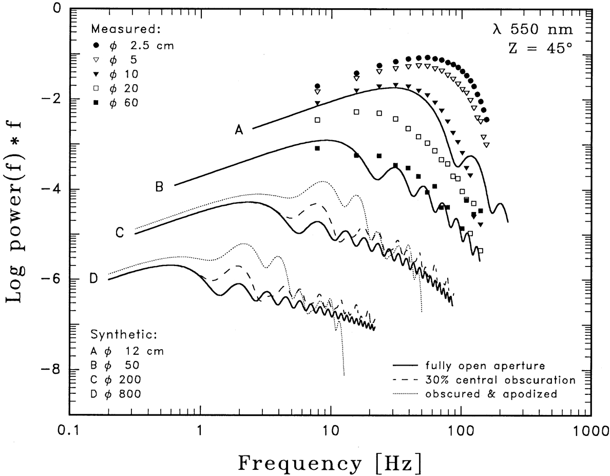
Fig. 2.— Power spectral content of scintillation in different apertures, i.e., the amount of integrated power, as a function of frequency. Observations and simulations are as in Fig. 1. This illustrates where in the spectrum the power is located. For smaller apertures, the power distinctly shifts toward higher frequencies. This trend continues until aperture diameters ø≲5 cm, where the structures in the "flying shadows" begin to get resolved.
Figure 2 shows that the power is mainly concentrated around the "knee" of the curves. This, apparently, is what led early observers of scintillation to try to describe it in terms of a single dominant frequency, or number of crossings of the mean value per second.
The data of Figures 1 and 2 permit a comparison of the scintillation levels on La Palma with those reported at other observatories. This will be discussed in § 7 below, but we note now that scintillation at major observatories appears to be rather similar.
4. CIRCULAR AND ANNULAR APERTURES
Scintillation measured through a telescope reflects the integration of the flying‐shadow pattern over the telescope's entrance pupil. If this pupil is somewhat irregular or complex, there will be a corresponding signature in the exact scintillation properties. In this section we examine scintillation properties in fully transmitting apertures with rotational symmetry.
4.1. Wind Speed Reflected in Scintillation
Not only optical but also acoustic and radio waves can be used to remotely infer properties of winds that are crossing the line of sight, in either the lower atmosphere, the ionosphere, the solar wind, or even the interstellar medium. This is done by observing the drift of the scintillation pattern that is produced when refractive‐index inhomogeneities are carried across the line of sight; different techniques are discussed by, e.g., Monastyrnyi & Patrushev (1988) and Wang, Ochs, & Lawrence (1981). Such methods naturally assume the Taylor hypothesis of local frozenness of inhomogeneities, so that observed changes are due to their transport by the wind rather than to intrinsic evolution.
An understanding of such effects is a prerequisite for understanding differences in scintillation between different telescopes and how to optimize the entrance pupil in order to enhance its sensitivity for detection of various time‐variable phenomena. We now examine some theoretical calculations, showing the response to changing position in the sky, to varying wind speed, or to introducing a central obscuration (such as arises from the secondary mirror in ordinary reflecting telescopes).
4.2. Synthetic Autocovariances
Synthetic scintillation was computed, following the scheme in § 2.3. Synthetic (rather than observed) data are required for this discussion, in order to show the fine structure of specific aperture effects in a noise‐free manner.
The curves in Figure 3 show synthetic autocovariances at 550 nm, illustrating (1) the effects of altitude and azimuth and (2) the effects of increasing telescope size and introducing a central obstruction. Although this figure contains synthetic data only, both its amplitude and its timescale were fitted to empirically determined values for summer conditions on La Palma. All the curves have nearly the same shape: a big main lobe (shaped much like the modulation transfer function of the aperture), followed by a very weak negative tail, which monotonically approaches zero.
Fig. 3.— Scintillation autocovariances, showing dependence on wind direction (position on the sky) and on central obscuration (secondary mirror). For a circular and open 20 cm aperture, the function is shown for the zenith, and for two wind‐azimuth angles at zenith distance Z = 35°. The scintillation in a 2.5 m telescope is much less but shows somewhat complex time structure, caused by its 90 cm secondary mirror. The plot shows autocovariance + , where = 0.0002 for the smaller and 0.00003 for the larger aperture. The true zero levels (=) are marked. Although this figure contains synthetic data only, both amplitudes and timescales were fitted to empirically determined values for summer conditions on La Palma.
4.2.1. Circular Apertures with Clear Transmission
In Figure 3, there are three curves for the same circular (fully transmitting) aperture of 20 cm diameter. One is for observing in the zenith, and two are at different wind‐azimuth angles at zenith distance Z = 35° (1.22 air masses).
Note the azimuth effect away from the zenith. When looking along the projected wind vector, the shadow pattern's motion is foreshortened. This makes the projected motion slower than the wind speed. When looking at right angles to the wind, we see the full wind speed in the motion of the shadow pattern. In either case, the total variance in the shadow pattern is independent of the speed of motion, so the slower apparent motion along the wind corresponds to a greater power density at low frequencies; the integral of the power spectrum (the total variance) depends only on zenith distance.
The two curves at Z = 35° are simply separated by the projection factor for the effective wind speed; this scales as sec Z. The difference between the along‐wind and cross‐wind plots is due to this difference in projected wind speed (and not, e.g., saturation effects).
4.2.2. Effects of a Central Obscuration
Figure 3 also illustrates the effects of size and central obstruction, comparing the previous curves with a larger annulus; a 2.5 m telescope with a 90 cm central obscuration (secondary mirror) is shown. The 20 cm aperture is essentially in the geometric‐optics regime, so diffraction effects are negligible; the change in the shape of the curve, in going to the annular aperture, is due to the central obstruction. The amount of scintillation in the latter case is much less but also shows somewhat complex time structure, caused by the secondary mirror.
Examining the features for annular apertures, one notes that they show a shoulder, or (for narrower annuli) even a secondary maximum. As a patch in the shadow pattern drifts across first one side of the annulus and then the other, the autocovariance of the scintillation time series ought to show features rather like the autocorrelation of the aperture with itself—namely, its modulation transfer function (MTF). There is also some similarity to the MTFs of annular apertures; some differences arise because the spatial‐frequency content of the shadow pattern introduces a certain weighting. Since the scintillation power spectrum is a smeared version of the telescope's MTF (diffraction pattern), a central stop increases the high‐frequency scintillation.
For further discussions of the effects of central obscurations, see Young (1967). The central stop in typical telescopes obscures about 1/3 of the aperture and approximately doubles the high‐frequency contribution. Larger obscurations cause greater effects. Such increased high‐frequency scintillation may complicate the comparison of scintillation data between different telescopes.
Also, other obstructions in the telescope pupil, such as the spider vanes commonly holding the secondary mirror, will affect the amount of scintillation at some accuracy level (as well as the image quality through diffraction). For a discussion of the effects of secondary‐mirror spiders on the diffracted image, see Harvey & Ftaclas (1995); the relevance for scintillation follows from the relationship of the aperture‐filtering function with the telescope diffraction pattern.
5. APODIZED APERTURES
The previous section illustrated how the scintillation signal becomes enhanced by the presence of a sharp shadow from a telescope's secondary mirror. The mechanism can be readily understood; the presence of small and sharp structures across the entrance pupil has the effect of more abruptly extinguishing flux contributions from the flying‐shadow patterns, as these cross the aperture edge. Such sudden changes of intensity cause "ringing" and introduce more scintillation power at high temporal frequencies.
In this section we will analyze the opposite effect, namely, how the scintillation signal may be depressed in entrance pupils without any sharp edges. Flying shadows that cross the "fuzzy" (apodized) edges of such apertures, will experience only a gradual extinction, thus causing less scintillation power at high temporal frequencies.
5.1. Apodization of Astronomical Telescopes
Apodization of astronomical telescopes has been attempted in some instances, mainly for the purpose of imaging faint sources near stronger ones. By suitably modifying the radial transmission profile of the telescope's entrance pupil, the amount of diffracted light at certain distances from the center can be minimized. For example, the review by Jacquinot & Roizen‐Dossier (1964, their § 9.2.3) describes a telescope with an absorbing apodizer that was used to observe the faint white‐dwarf companion near Sirius. Other efforts are described by McCutchen (1970), Papoulis (1972), and Suiter (1994, p. 160). Apodization has other applications for coherent (laser) imaging and beam‐propagation systems (e.g., Mills & Thompson 1986).
5.2. Theory of Apodization Effects
The potential for using apodized telescope apertures to truncate high‐frequency parts of scintillation was discussed by Young (1967).
Apodizing a given telescope makes the central lobe of its diffraction pattern wider (this is the price for reducing the power in the tails). Since the aperture‐filter function for scintillation is of the same form as the diffraction pattern for imaging, an apodized aperture will always show more total scintillation than an unapodized one. The aperture becomes effectively smaller, and its power spectrum resembles that for a smaller sharp aperture. However, well out in the high‐frequency tail, the spectrum may fall steeply enough that the scintillation power becomes rather lower than with a sharp aperture.
An optimized apodizing function that falls off suitably fast for the desired higher frequencies may in principle be chosen. Although one could greatly depress the highest frequencies, a practical limit comes from the rapidly diminishing aperture transmission; as the apodization increases, so does the photon noise. Also, there are limits as to how precise apodizing filters can be practically made (as opposed to mathematically idealized ones). For the optimum apodization of an obstructed aperture (e.g., a telescope with a secondary mirror), one should smooth both the inner and outer aperture edges.
We will only consider apodizers with smoothly variable transmission at their edges. Also, "apodizers" with sharp edges (at special oblique angles) have occasionally been used in, e.g., spectroscopy. However, these introduce more high frequencies from flying‐shadow components in these oblique directions.
5.2.1. Apodizing in Only One Dimension
Since the purpose of apodization is to match the spatial crossing of the flying shadows across the aperture edges, and the shadows often have a preferred direction of motion, apodization in only one coordinate, i.e., in the direction of the flying‐shadow motion, might be sufficient (Young 1967). In the case of a rectangular aperture, and wind along x, there will be no benefit from apodizing also perpendicular to x. However, the mask must be aligned very closely along the wind direction, which thus should consist of a single component. Otherwise, there enters some projection of the unapodized coordinate along the wind, and the tail of the temporal power spectrum eventually assumes its unapodized form.
In the case of a single wind component, fluctuating only in angle, one could even conceive of adaptive apodization filters, correcting for the changing angle in real time (cf. § 7.4); however, the required stable and simple wind patterns might not be encountered very often. Measured wind vectors typically fluctuate several degrees over a few minutes (§ 6), and in practice rotationally symmetric apodizing masks appear more useful, being an "insurance" against wind‐direction variations.
5.3. Apodized Apertures on La Palma
Although the scintillation theoretically expected in apodized apertures has thus been previously discussed, there appear not to exist any previous measurements thereof in the literature.
A series of scintillation observations were therefore made on La Palma using various apodized telescope apertures. These were achieved by covering openings in front of the telescope with suitably prepared films of glass‐clear thin polyester film (6 μm thick Mylar®). The outer rims of these films were painted in an airbrush studio to generate differently "fuzzy" edges.
Four such circular apertures of 20 cm diameter were mounted in front of the 60 cm telescope, in a pattern to avoid any shadowing from either the secondary mirror or its support. Three apertures had various levels of apodization; all had a clear center and a gradual decrease of transmission from unity to zero, starting at radial positions ≃7.5, 5, and 2.5 cm from the center, out to the full radius of 10 cm. For calibration, the fourth aperture was a completely clear one, covered with an otherwise identical film. As for other telescope apertures, a change between any of these could be made in a few seconds, by remotely operating a shutter.
Figure 4 shows the radial optical transmission in two of the apodized ø = 20 cm apertures used, as measured in white light on a PDS microphotometer. Possibly, an "ideal" apodization mask should have a Gaussian run of amplitude transmission; something akin to such a dependence had been aimed at.
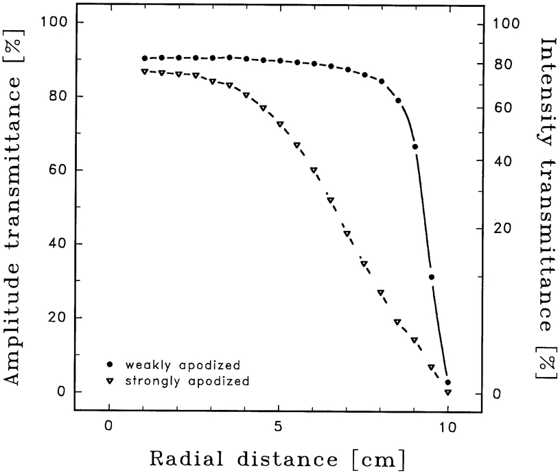
Fig. 4.— Transmission profiles of apodization masks used on La Palma. These "unsharp" telescope apertures were made from airbrush‐painted Mylar® films. The radial dependence of optical transmission in two of these is shown, as measured on a microphotometer. The amplitude scale (left) is relevant for computing diffractive effects of light, while the scale at right is the ordinary light intensity.
Some further experiments were made for the full ø = 60 cm aperture (with its central ø = 17 cm secondary mirror obscuration). Another sharp mask had the central obscuration enlarged to ø = 40 cm (to enhance scintillation), while another was apodized at both its outer and inner rims (adjoining both the primary and secondary mirror edges), as well as along the locations of the spider vanes, thus removing all sharp edges from the entrance aperture. The positioning of this mask over the spider vanes was made by examining the (extrafocal) image of the telescope's entrance pupil.
Of some concern was the quality of the resulting stellar images, as seen through these Mylar® films. When examined through an eyepiece at high magnification, the stellar images could be seen to expand farther out than without such masks (to some ≃5 '' diameter, still much smaller than the ≃1 ' field of view) and were somewhat "streaky," but otherwise sharp and crisp. Such films have been used also by other experimenters to enclose telescopes (Thompson 1990; Borra et al. 1992), verifying that, with careful mounting, such thin films indeed permit very good (nearly diffraction‐limited) image quality.
5.4. Observations through Apodized Apertures
Results from our measurements are shown in Figure 5 for autocovariances, and in Figure 6 for power spectra. For clarity, only data for the "sharp" and the most strongly apodized aperture are shown. The "sharp" one is thus a fully clear ø = 20 cm Mylar® window of the same material used for the ø = 20 cm "apodized" one (corresponding to the "strongly apodized" curve in Fig. 4). These figures also show corresponding theoretical curves, computed as described in § 2.3.
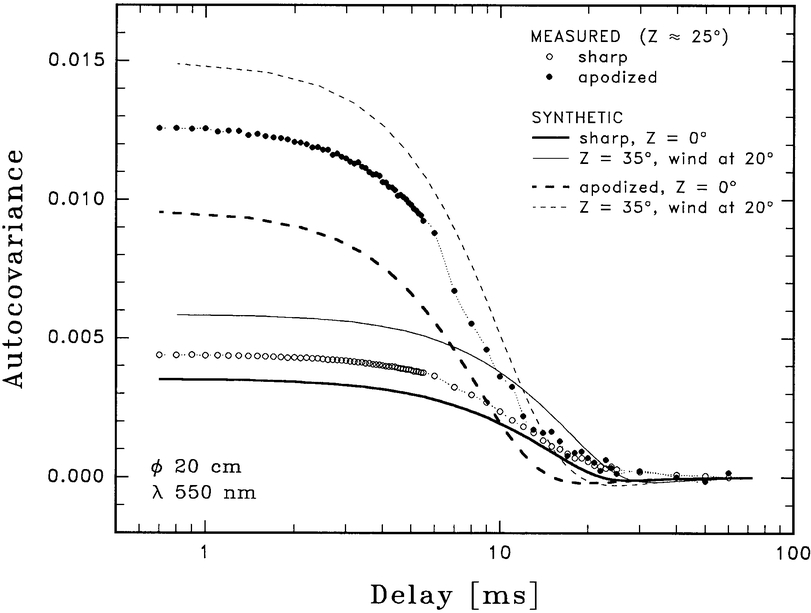
Fig. 5.— Measured and synthetic autocovariances for sharp and apodized apertures. The "sharp" one is a clear Mylar® window of similar material to the "strongly apodized" one (Fig. 4). The increased autocovariance (power) for the apodized aperture is caused by its smaller effective diameter (due to its apodized edges), mimicking a smaller sharp aperture. The differences at the highest frequencies are seen in Fig. 6.
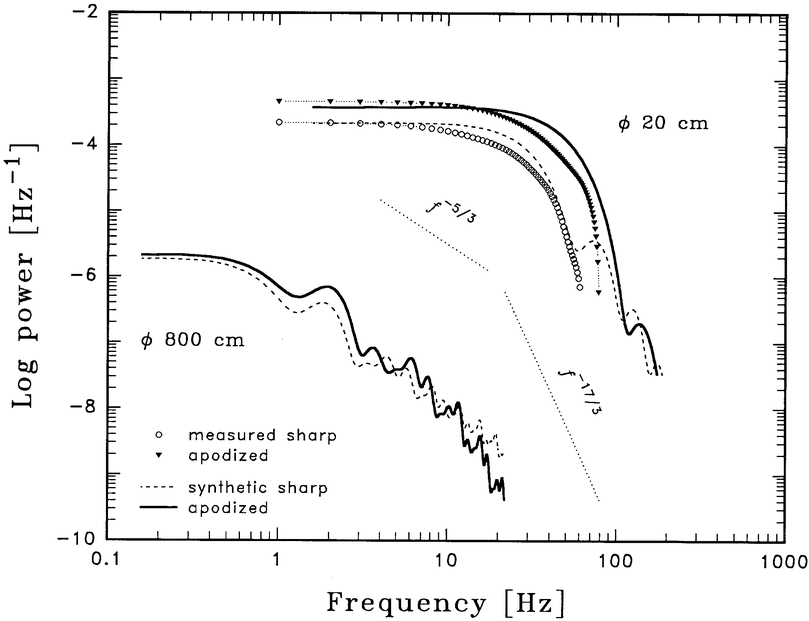
Fig. 6.— Measured and synthetic scintillation power spectra for sharp and apodized apertures. As in Fig. 5, the increased power at most frequencies for the apodized aperture originates from it being effectively smaller. However, for the highest frequencies, there is a tendency for the spectrum to fall off steeply enough, that the power seen with the apodized aperture becomes less than with the clear one.
All observations are from good summer nights on La Palma, measuring Vega at typical zenith distances Z ≃15°–20°, or Deneb at Z ≃20°–25°;λ = 550 nm. Autocorrelations were recorded with sample times 0.1 and 1 ms, rapidly switching between the four different ø = 20 cm apodized and clear apertures. To calibrate the aperture‐size dependence, also sharp apertures bracketing the apodized ones in size were measured during the same nights (ø = 20, 14, 10 cm).
A total of more than 200 autocorrelation functions were thus recorded. The main uncertainty in the reduced data is believed to stem from occasional difficulties of merging autocorrelation functions, recorded at different epochs, and with different time resolutions.
The actual wind speed differs somewhat from night to night; its value is deduced in the fitting of synthetic functions to observed data points. For the data in Figure 5, an overhead wind speed of 8.7 m s−1 was obtained, versus 9.6 m s−1 for Figure 6. Synthetic curves are given for two zenith distances:Z = 0° and Z = 35° (assuming a plausible wind azimuth). The two synthetic curves thus bracket the observed points (Z ≃25°) with respect to zenith distance.
Figure 5 shows autocovariances versus temporal delay, comparing model calculations with data. The data and models agree well for delays less than about 15 ms. At longer delays, there seems to be more variance than expected, and it is similar for both sets of data, apodized and sharp. As it seems to exist for long lags only, one suspects a low‐level layer of turbulence with slow wind speed, on the order of 5 m s−1.
The main effect seen in Figure 5 is that of increased autocovariance (power) for the apodized aperture. This originates from that aperture being effectively smaller, so its total power and "knee" frequency look like those of a smaller sharp aperture (e.g., they fall to half the peak value at a smaller time lag). All the curves have a big main lobe, followed (in synthetic data) by a very weak negative tail.
More interesting apodization effects show up in the high‐frequency tails of the power spectra, beginning to get visible in Figure 6. As in the autocovariances, the increased power at most frequencies for the apodized aperture originates from that aperture being effectively smaller. However, for the highest frequencies, the tendency is to make the spectrum fall off steeply enough that the power with the apodized aperture is less than with the clear one: the curves cross around 100 Hz. Straight lines with slopes of f−5/3 and f−17/3 show the theoretically predicted runs of scintillation power in the high‐frequency tails for sharp and apodized apertures, respectively (§ 2.3.3). Figure 6 also shows the predicted scintillation in sharp and apodized 8 m telescopes (with ø = 2.4 m central obscurations), normalized to the scintillation power observed on La Palma, indicating the lowest levels of scintillation that realistically can be obtained in single telescopes at such sites.
Some other measurements did not produce convincing differences between sharp and apodized cases. With the large ø = 60 cm apertures, very short timescales (down to 1 μs) were also examined, searching for effects at very high frequencies. Another search was for possible wavelength dependences between 365 and 700 nm. The analysis of these measurements remained inconclusive because of the difficulty of segregating effects of effective aperture size from those of apodization proper.
5.5. Differences among Ordinary Telescopes
Synthetic scintillation was computed for various telescopes with primary and secondary mirror sizes typical of those at major observatories. Figure 7 shows the spectral power density for five different 2.5 and 3.5 m telescopes: with and without central obscurations; with and without apodization. Although this figure contains synthetic data only, both the amplitudes and timescales were fitted to empirically determined summer values for La Palma, normalized to Z = 45° and λ = 550 nm.
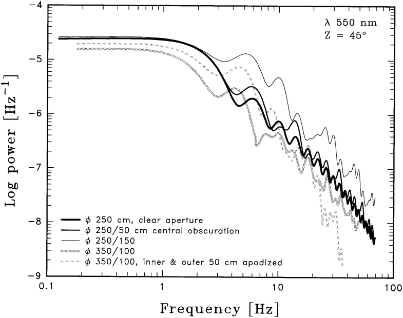
Fig. 7.— Synthetic power spectra for apertures with and without central obscuration, and with and without apodization. The scintillation power at 10–100 Hz may differ by an order of magnitude between telescopes that otherwise would appear to be nearly equivalent. For investigations that are limited by atmospheric effects, this shows the potential for improving sensitivity by optimizing the geometry of the telescope's entrance pupil. These synthetic data were normalized to observed summer conditions on La Palma, in both power and frequency.
The main point shown in Figure 7 is that the power at "typical" scintillation frequencies of 3–30 Hz may differ by a whole order of magnitude between telescopes that otherwise would appear to be nearly equivalent.
The three models for a 2.5 m telescope are for a fully clear aperture, for a small secondary mirror of 50 cm diameter, and for a very large one of 150 cm. The two models for a 3.5 m telescope have a secondary obscuration of 100 cm, one telescope with sharp edges, and another with the annular aperture apodized at both the inner and the outer edges.
The general features seen are (1) increased high‐frequency content for apertures with large central obstructions; (2) same asymptotic slope in the high‐frequency tail for all sharp‐edged apertures; (3) increased low‐frequency but decreased high‐frequency power for the apodized aperture (and hence a steeper power law in the apodized tail); and (4) beats between the Bessel functions for the inner and outer circles of the annular apertures.
Apodizing both inner and outer edges significantly enhances the scintillation in the lower frequency "knee" region but produces order‐of‐magnitude reductions at 100 Hz and beyond. Such large effects require apodizing both edges; apodizing only the outer one reduces the high‐frequency tail by only about a factor of 2. As long as the aperture still has one sharp edge where the light is cut off discontinuously, there will always be a tail with the −8/3 power (until diffraction and inner‐scale effects take over; § 2.3.3). But the aperture with all edges apodized has a filter function that falls off as f−6 instead of f−3. Thus, the tail for the apodized aperture falls as f-(8/3 + 3) or f-17/3.
5.6. Laboratory Experiments
Not everything involving apodized apertures is completely clear. Since previous astronomical observations appear to be lacking, and our own La Palma measurements were necessarily limited in types of apodization masks examined (as well as in measuring precision), a number of supplementary optical experiments were made in the laboratory.
A number of apodizing filters were made by an optical company. These glass filters (of physical size ø = 2.5 cm) had clear centers and different runs of apodization at their edges. They were mounted on an optical bench, where the optics imaged these as entrance pupils for a simulated telescope.
Such types of filters might be incorporated into an astronomical photometer. Their function would be to mask off the entrance pupil (reimaged onto that filter), thereby damping the high‐speed scintillation. Questions that arise include, e.g., whether the same "filter" would be optimal also if we used the same photometer on a telescope of another size (quite apart from the question of different secondary mirror obstructions). Could the extent of the apodization edge be optimized to match the different speeds of the flying shadows?
Laboratory experiments were made by simulating stellar observations through telescopes with different effective levels of apodization. Starlight was simulated by a pinhole, and the flying shadows were produced by a transparent rotating mask, with irregular patches painted onto it. Both the apodized filter and this painted mask were thus imaged onto the detector. Varying the speed of rotation for this mask simulated various speeds of the flying shadows. The signal was measured with similar detectors and data‐handling electronics as used on La Palma. Resulting power spectra were computed and comparisons made between those measured through sharp and through differently apodized apertures.
Although these experiments were incomplete as concerns, e.g., the more detailed simulation of scintillation (shape of its power spectrum, modulation only in one spatial coordinate, etc.), they did bring some insights into the possibilities (and problems) of apodization. The experience will be applied in the discussion of optimal observing techniques in § 7 below.
5.7. Other Effects from Apodization
Introducing apodized apertures may cause other, perhaps unexpected, effects. The spatial and temporal coherence of light in general cannot be separated, as both contribute to its degree of coherence. However, that can sometimes be expressed as the product of the degrees of spatial and temporal coherence; in such a case the light is cross‐spectrally pure.
Effects from atmospheric turbulence include both phase changes (image "boiling") as well as an overall transition by the flying shadows. For "boiling" only, the spacetime intensity correlation of stellar speckle patterns in the image plane is cross‐spectrally pure, i.e., the correlation may be written as the product of a space‐only part and a time‐only part. In the case of flying shadows moving across also, this is no longer true, except for an apodized aperture with a Gaussian amplitude transmittance. Thus, certain correlations being reported for stellar speckle patterns are apparently specific to the use of sharp telescope apertures (Dainty, Hennings, & O'Donnell 1981; Jakeman 1975; Jakeman & Pusey 1975; O'Donnell, Brames, & Dainty 1982).
6. DOUBLE AND ELONGATED APERTURES
The sharp and apodized apertures hitherto used were all circularly symmetric. We now turn to asymmetric apertures: elongated, double, or multiple. Such apertures perceive a different scintillation signal, which permits the determination of additional properties for the components of the flying‐shadow pattern, e.g., their respective velocities.
Although double or elongated apertures are not common among optical telescopes, there are exceptions, with two or more mirrors on the same telescope mount. Also, the equivalent signal can be obtained by combining data from two nearby but separate telescopes.
6.1. Previous Studies
The information content of noncircular apertures was realized early, once the flying‐shadow nature of scintillation was accepted. Mikesell et al. (1951), Mikesell (1955), and Protheroe (1955a) used slitlike apertures of adjustable width and orientation to find the dominant wind direction. The slit was rotated, monitoring the high‐frequency power component of scintillation. The position angle for its minimum value indicates the direction of flying‐shadow motion (high‐frequency scintillation with the slit along that direction should be similar to that in a large aperture, whereas in the perpendicular position it should resemble observations in a small aperture; cf. Young 1969).
More quantitative studies are possible through double (or multiple) apertures, i.e., ones where the entrance pupil consists of two discrete openings at some distance from another. In particular, the temporal correlation can be studied between small apertures across the pupil plane, for the purpose of deducing atmospheric properties (Rocca, Roddier, & Vernin 1974).
6.2. Measurements on La Palma
For our experiments, an aperture mask with three pairs of sharp apertures was placed over the telescope. Each individual aperture was circular, ø = 10 cm, and the apertures were spaced by 20, 30, and 45 cm, center‐to‐center. Any one of these pairs could be quickly selected for observation (or else one single aperture), and the position angle for the two apertures could be rapidly adjusted by rotating the aperture mask.
The observations involved autocorrelations and probability‐density functions as before, but in general with shortened integration times, necessitated by the additional degrees of freedom available (both aperture spacing and position angle). As seen below, a characteristic signature comes from the flying‐shadow direction and speed. During stable summer conditions, reproducible signatures did occasionally remain during 20–30 minutes, i.e., there was then no significant change in either the apparent wind speed or direction. On other occasions, however, significant shifts were noted in 5 minutes or less. Such rapid changes preclude long integration times for decreasing random noise (or the averaging of many data records), since that washes out the flying‐shadow signatures. As a compromise, integrations were normally kept to 50 s, and the position angle was changed in steps of 30° or 60°.
The intensity autocorrelation seen through a double aperture is quite different from that in a single one. Also, the structure of its main peak may change very significantly with position angle; a secondary peak is usually reproducible, but only within a rather narrow range of angles. Figure 8 shows a selection of representative measurements through various double apertures.
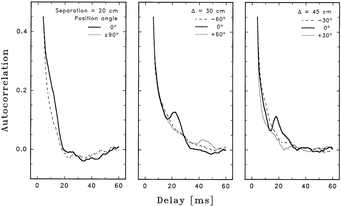
Fig. 8.— Scintillation measured through masks with two ø = 10 cm apertures, at different separations and position angles. If the same flying‐shadow pattern crosses both apertures, a secondary peak appears in the autocorrelation, revealing the flying‐shadow speed and direction. The autocorrelation changes significantly with position angle; the secondary peak is reproducible only within a rather narrow range (≃30°). For apertures separated by 30 cm, typical delays of 20 ms indicate a flying‐shadow speed of ≃15 m s−1.
These measurements of Deneb (at Z ≃ 25°–35°) were made at 550 nm. The (ground) weather conditions were noted as typical good summer weather on La Palma—relatively strong, stable northerly wind. The autocorrelation sample time was 1 ms, and each curve in Figure 8 is the average of two records.
A sequence of position angles was measured in a nonmonotonic sequence, identifying the angle corresponding to the (temporary) direction of the dominant wind. For a 30 cm spacing, reproducible secondary peaks usually appeared within a position‐angle interval of ≃30°. Following such a determination, a sequence of measurements for different aperture‐pair spacings, or at different wavelengths was made, keeping the position angle fixed (Figs. 8 and 9). This reference angle is denoted 0°. That direction could easily change by ±60° during a night, and ±30° in 15 minutes. In such a time, also the delay‐time position for the secondary peak might shift by a factor of ≃2.
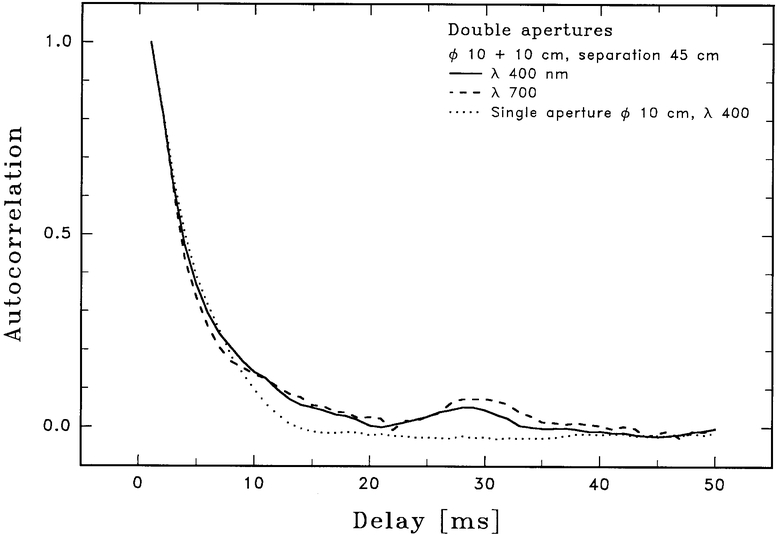
Fig. 9.— Double and single apertures, and different colors. Autocorrelations were measured through a mask with two ø = 10 cm apertures, separated by 45 cm. The position angle was adjusted to show a secondary peak due to flying shadows crossing at a speed of ≃15 m s−1. This secondary peak remains essentially unchanged between λ = 400 and 700 nm, but the function is strongly different from that seen in a single 10 cm aperture.
6.3. Wind Speed(s) and Position Angle(s)
If the same flying‐shadows pattern passes both apertures, a secondary peak appears in the autocorrelation. (A small shadow element in linear motion will cross both apertures for angles ≲arcsin [D/Δ], with D the diameter of each aperture and Δ their center‐to‐center separation.) From the spacing, and the orientation of the aperture pair, the speed and direction of the flying shadows can then be determined. Figure 8 shows how such a second maximum is well resolved when the apertures are well separated, but only appears as a slight convexity on the curve when the apertures are close together.
Wind speeds can be derived from the time lag at the secondary peak, when the apertures are aligned along the wind; for example, the middle panel shows a maximum at ≃23 ms for 30 cm separation, so the projected wind speed is 30 cm/23 ms, or ≃13 m s−1. For a more exact calculation, using observations away from the zenith, the precise geometry of the apertures must be accounted for. If these are aligned vertically above one another, and one is looking into the wind direction, the effective distance between the apertures, as projected onto a horizontal surface, is increased by a factor sec Z (here ≃1.15) compared to the value in the pupil plane.
Occasionally, multiple wind components could be recognized, showing contributions from multiple layers of turbulence with different wind vectors. The middle‐panel curve for +60° shows such a peak around 45 ms, indicating that the wind speed in that particular atmospheric region was about half as great as in the main one, and directed ≃60° away from its particular wind vector.
The width of the secondary peak corresponds roughly to the size of the individual apertures; it remains unresolved when the apertures are close together (Fig. 8, left) but is clearly resolved for the wide separations. Its contrast improves markedly on going from 30 to 45 cm separation.
Figure 9 shows that the autocorrelation function in double apertures does not sensibly change with optical wavelength but is strongly different from that seen in a single ø = 10 cm aperture. After adjusting the position angle to show a stable secondary peak (here corresponding to a shadow speed of ≃15 m s−1), a sequence of measurements was made in rapid succession. For the double aperture, rapid switching between 400 and 700 nm filters was performed, intermingled with measurements through the single aperture at 400 nm.
7. AVOIDING SCINTILLATION EFFECTS
In astronomical observations, scintillation normally constitutes a noise source to be avoided. For larger telescopes (low‐frequency) scintillation is the dominant noise source for photometric broadband measurements of stars brighter than mv ≃12 or 13 near the zenith (assuming detectors of high quantum efficiency; e.g., Gilliland et al. 1993). At large air masses, the crossover to photon noise as the dominant one occurs at a few magnitudes fainter. Scintillation also hinders highest definition imaging, since the irregular illumination pattern caused by the flying shadows diffracts into the wings of focused stellar images.
Until now, we have treated scintillation as a physical phenomenon to be studied. In this final section concluding our series of papers, we will, however, instead view it as a noise source to be avoided, and exploit the understanding gained of its properties to define schemes for optimally circumventing its effects in astronomical observations.
7.1. Optimum Observing Sites
An obvious variable is the location of the telescope, ideally placed in space. That indeed avoids effects of the terrestrial atmosphere, but instead introduces numerous other problems. The most ambitious effort so far to thus avoid scintillation was the High Speed Photometer on the Hubble Space Telescope. Several other photometry missions have been proposed (aiming at micromagnitude precisions) and their concepts studied by different space agencies.
Observatory site testing has most often been made to find locations with advantageous seeing conditions, producing sharp images. However, some high‐altitude sites have also been examined for scintillation: Jungfraujoch (Siedentopf & Elsässer 1954); Pamir (Darchiya 1966), sites in Armenia, the Andes, and Pamir (Alexeeva & Kamionko 1982), Mauna Kea (Dainty et al. 1982), Mount Maidanak (Gladyshev et al. 1987), La Silla and Paranal (Sarazin 1992, and 1997, private communication1). However, only rather small differences are seen in scintillation amplitudes between sea‐level and mountain sites (although great differences exist in the seeing). This is understandable since scintillation originates at large atmospheric heights and (in contrast to seeing) is not much influenced by local conditions or by low‐level topography. Scintillation monitoring reveals how the characteristic timescales undergo seasonal changes, corresponding to those in high‐altitude winds (Sarazin 1992, and 1997, private communication).
7.1.1. Searching for Optimal Timescales
The origin of scintillation in high‐level turbulence and its correlation with high‐level winds suggests that slower scintillation can be expected at sites with relatively slow high‐level winds. Many major observatories (Canary Islands, Chile, Hawaii) are located at latitudes with rapid overhead jet streams. This appears to imply rapid scintillation and (with more kinetic energy available to produce turbulence) a greater amplitude. On dimensional grounds, the turbulence strength should be proportional to the kinetic energy in the wind, as confirmed for at least some combined measurements of (low‐frequency) scintillation and wind speed (Young 1969, his Fig. 20).
Parameters that relate to scintillation are those of the lifetime and temporal correlation of speckles inside focused images. Such quantities are being studied to assess a site's suitability for speckle‐ and other types of interferometry. Those timescales are coupled with the time for the phase and intensity distribution in the telescope aperture to change significantly, and thus are related to scintillation parameters. Often, two distinct timescales are seen: one short (≃2–10 ms) associated with the boiling of the speckles within the image, and a much longer component of image motion, i.e., the random motion of the speckle‐image envelope.
On Mauna Kea, the variability of speckle lifetimes during and between nights appears to be significantly higher (factors of 5 or more: Dainty et al. 1982; O'Donnell et al. 1982) than at other sites (factors of 2–3): Herstmonceux, England (Scaddan & Walker 1978; Parry, Walker, & Scaddan 1979), Haute‐Provence (Aime et al. 1986), La Palma (Dainty, Northcott, & Qu 1990), or La Silla (Vernin et al. 1991). Also, at Paranal there are indications for rapid variability of speckle lifetimes (M. Sarazin 1997, private communication). These differences could be due to the proximity of Mauna Kea and Paranal to main jet streams, one reason for the otherwise excellent weather these sites are enjoying.
For finding regions with low wind speeds for scintillation, global maps for, e.g., the 200 mb atmospheric level (≃11 km altitude) may be examined (Vernin 1986). The wind maxima are along ±30° latitude (where many major observatories are located, due to the large number of clear nights), while the minima are near the equator and near the poles. In response to concerns about the short timescales, and their ensuing problems for interferometry and adaptive optics, some site testing has been done on candidate sites with expected low wind speeds, such as Réunion in the Indian Ocean. However, equatorial sites can be problematic because of frequent or seasonal clouds, but perhaps Antarctic sites might be feasible.
7.1.2. Airborne Observing
Observatory "sites" with the most rapid wind conditions are found on board airplanes. The effective wind speed of ≃250 m s−1 means that the shadow pattern crosses the telescope an order of magnitude faster than usual. By itself, this does not change the total amount of scintillation, but rather has the effect of shifting the scintillation spectrum to much higher temporal frequencies, and spreading its power over a wider frequency band.
The seeing conditions for such observing were examined by Zwicky (quoted in Oosterhoff 1957), but more quantitative data were obtained by Dunham & Elliot (1983). Comparing ground‐based data to photometric measurements made with a 90 cm telescope on board the Kuiper Airborne Observatory, they found the major difference to be "the absence of scintillation" and large (≃5 '') images. The latter is probably caused by the boundary layer of the aircraft. The low level of scintillation is consistent with it originating from distant sources: when already flying at the tropopause level, the optical effects from the turbulence remaining at very high levels are tiny.
The generally lower scintillation level, combined with its shift to higher frequencies, can be exploited for various photometric tasks, including the observing of lunar or planetary occultations of stars. Larger‐size airborne telescopes, such as the 2.5 m one currently being built for SOFIA, are likely to offer very low scintillation levels.
7.1.3. Photometric Performance of Different Sites
Theoretical considerations provide an approximate scaling law for the rms error due to the low‐frequency component of scintillation (Young 1967, 1974):

where D is the aperture diameter in centimeters, sec Z is the air mass, h is the observer's height above sea level,h0 ≃8000 m is the atmospheric scale height, and T is the integration time in seconds. The air mass exponent of 1.75 is an approximate value not far from the zenith; it equals 2 when looking along the wind direction and 1.5 perpendicular to it. The rms deviation σ is then obtained in units of relative intensity ΔI/I.
This expression applies for timescales longer than those for flying shadows to cross the telescope aperture, i.e., integrations on scales of seconds and longer. (More strictly, for frequencies below V⊥/πD, where V⊥ is the speed at which turbulence crosses the line of sight and D the diameter of the telescope, ≃10 m s−1/10 m = 3D 1 Hz for telescopes in the 2–3 m class.) When incorporating also the high‐frequency part of scintillation, the aperture dependence is steeper (eq. [1]). However, it is the low‐frequency power in equation (10) that is perceived as noise in ordinary photometry, and "limiting" accuracies for ground‐based photometry can be estimated from this expression (Brown & Gilliland 1994; see also Young et al. 1991; Gilliland & Brown 1992; Kjeldsen & Frandsen 1992; Heasley et al. 1996).
From various observing campaigns it is possible to compare the scintillation levels at different observatory locations. Although the precise amount of scintillation of course changes from night to night, the scaling law (eq. [10]) appears to hold quite well for apertures up to at least 4 m, and for quite different sites (Kjeldsen 1991; Gilliland & Brown 1992; Gilliland et al. 1993).
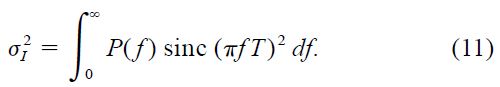
Our data for the power spectral density measured on La Palma can be used to calculate the scintillation noise expected in photometric integrations. The intensity variance for a given integration time T can be computed from the power‐density spectrum P(f) through the integral
In the case T = 0, one obtains
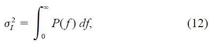
which is the relation used earlier to normalize P(f).
For large T, the expression may be approximated by setting P(f) = P(0) for f<1/T, whereupon P can be taken outside the integral:
Applying this for our power spectra in Figure 1, we find P(0) ≃1.5 × 10⁻⁵ when interpolating to a 4 m aperture. This is for Z = 45°; scaling to the zenith by the factor (sec Z)3 gives ≃5 × 10⁻⁶. For an integration T = 60 s, we then find a σ on the order of ≃200 μmag, quite comparable to near‐zenith values measured on 4 m class telescopes on Kitt Peak and Mauna Kea (Gilliland et al. 1993).
7.1.4. Antarctic Locations
There might conceivably exist some ground sites with exceptional scintillation properties. Sites in Antarctica appear to be particularly promising, although these have as yet been only incompletely examined.
Potentially unique scintillation properties might exist at high‐altitude sites (≳4000 m) on the plateau in East Antarctica (see, e.g., Burton 1995). Here the equivalent pressure altitudes in winter are in excess of 5000 m. The geomagnetic latitude of some potential sites (e.g., Dome C at 73° S, 127° E) places them close to the center of the auroral oval, making the night sky much darker than at the South Pole.
Of probable relevance for scintillation is the circumstance that during most of the year, the tropopause at these sites, in effect, reaches the ground. The ground temperature is already very low and (except for a few summer months) the atmospheric temperature increases monotonically from the ground into space. The lack of significant thermal gradients leads to low wind speeds at all atmospheric heights; the wind systems are dominated by slow laminar air flows downwelling from the stratosphere, without any jet streams. The low kinetic energy content in the air mass limits the energy available to generate turbulence and mixing. Seeing data from various Antarctic sites suggest that there is significant turbulence only over the lowest hundreds of meters. While this causes some angular seeing, it should not much affect scintillation, since its dominant contributions come from distant (focusing) atmospheric layers.
Balloon‐borne microthermal sensors, measuring C2nup to some 40 km altitude, have verified the exceptional stability of the high‐Antarctic air mass. Heasley et al. (1996) discuss scintillation limits, and special sites, including the South Pole. They quote radiosonde data, from which C2nvalues are deduced, concluding that the intensity variance σ2I should be a factor of 5 smaller at the South Pole than at Mauna Kea, two sites at about equal equivalent pressure altitude. It appears likely that sites such as Dome C, at still higher altitude and with a quieter atmosphere, could be even better.
There could still be other problems, such as effects from blowing snow. Atmospheric transparency noise was measured at the South Pole by Duvall, Harvey, and Pomerantz (Harvey 1988). For frequencies ≳0.1 Hz, that is found to be very much smaller than scintillation noise, although it starts to dominate for fluctuations on scales of minutes and longer.
When discussing Antarctic sites, the difference between sites for good angular seeing and for low scintillation should be understood. Sites with excellent seeing could be exploited already with moderate‐sized telescopes in the 1 m class. Even if the seeing would be poor (presence of low‐altitude turbulence), a site could still be excellent for scintillation (Paper I). In contrast to telescopic image quality, however, scintillation noise significantly improves with increased telescope size; an Antarctic site would have to be enormously much better in order for a 1 m telescope, say, to compete with a very large telescope at an ordinary location. While moderate‐sized telescopes may be realistic to operate at these remote sites, the logistic problems suggest that very large telescopes will have to await the possible development of better infrastructure in the more distant future.
The potential of sites in Greenland has also been voiced, though it is not clear how good such sites could be, compared to Antarctica. Although elevations reach above 3000 m, it appears that Greenland is not big enough to create its own stable weather systems, as opposed to Antarctica.
As a general caveat about the scintillation to be expected at "exotic" sites, we want to stress that the atmospheric processes causing scintillation should be understood. As stressed in § 4.6 of Paper I, thermal stratification alone does not cause scintillation; there must be a wind shear to produce turbulence and mixing of air across, e.g., inversion layers (by themselves, such layers tend to suppress turbulence). Monographs introducing the relevant topics of atmospheric dynamics and boundary‐layer meteorology include Lumley & Panofksy (1964), Panofsky & Dutton (1984), Oke (1987), and Stull (1988). No matter how "promising" a site might appear, its quality should be verified by optical scintillation measurements.
7.1.5. Multiple Telescopes
Irrespective of geographical location, scintillation effects can be significantly reduced by combining the signals from several telescopes. At low frequencies, the scintillation‐noise amplitude σ decreases with the telescope diameter only as D−2/3 (eq. [10]). The telescope area is proportional to D2, so the noise amplitude decreases only as the cube root of this area. However, if instead of one large telescope, one uses several little ones with the same total area, the noise amplitude decreases with the square root of the number of telescopes (hence, the square root of the area).
To reduce (low‐frequency) scintillation noise by a factor of 10, using a single aperture, thus requires an increase of its area by a factor of 1000, or its diameter by over 30 times. The same gain can be obtained with an array of 100 small telescopes, whose signals are averaged together. If the construction of new telescopes is considered for projects where photometric precision is an important element, it must be noted that—since the cost of large telescopes increases at least as fast as their collecting area—a given capital investment will be much more efficient in terms of photometric noise if distributed over many small telescopes, rather than over a few larger ones.
To optimize the spatial distribution of the elements in such an array, the possible correlations among their individual apertures have to be evaluated. A calculation of the covariance shows that the scintillation in neighboring telescopes is weakly anticorrelated if they are within the atmospheric outer scale (believed to be on the order of 10 m, although deduced values differ greatly; § 6.7.2 in Paper I). The anticorrelation follows from the circumstance that, next to a bright structure in the atmospheric shadow pattern, there must follow a darker one, also manifest in the negative autocovariances in Figure 3. Thus, one can actually cancel out slightly more of the scintillation by placing the telescopes side by side. However, such gains can be only slight, because several telescopes placed side by side will in effect start making up one single large aperture. Time‐delayed correlations will enter for telescopes along the wind vector (partially) observing the same flying shadows (cf. Fig. 8). Probably, an optimum configuration has to be dilute enough to be pseudorandom, i.e., without regular spatial features—perhaps corresponding to a minimum‐redundancy array in ordinary interferometry. Since the likely gains from precise optimization are likely to be modest, we have not pursued these studies further.
This discussion applies to low‐frequency scintillation. Its high‐frequency component obeys other relations and will not be equally reduced by the measures discussed in this section (cf. eq. [1], Fig. 1).
7.2. Challenges in Photometry
There exist classes of astronomical observations that at present are hindered by scintillation, although some of them might be carried out from space. Besides the more obvious ones of rapid variability in compact astrophysical objects and other sources on subsecond timescales (Dravins 1994), there are also several phenomena on longer timescales.
These include challenges in asteroseismology, e.g., the photometric detection of stellar p‐mode oscillations in "ordinary" stars. The corresponding solar p‐modes have an intensity amplitude ΔI/I of perhaps ≃5 × 10⁻⁶ within a narrow frequency band, with periods around 5 minutes. The photon fluxes from stars would permit the observation of such oscillations as faint as about mv = 10, even without going to very large telescopes, but efforts are limited by scintillation (Harvey 1988; Gilliland & Brown 1992; Heasley et al. 1996).
Another example is stellar microvariability, e.g., in response to an evolving number of convective features (granules) on the stellar surface, corresponding to phenomena observed on the Sun (Rabello Soares et al. 1997). In the power‐density spectrum of the Sun, seen as a star, there are astrophysically significant signals down to levels below 10−8 Hz−1 at low frequencies, a few orders of magnitude below our scintillation power curves for very large telescopes in Figure 1.
Although, on longer timescales of minutes, other effects than scintillation proper also do enter, e.g., atmospheric transparency fluctuations, extinction anomalies, and other phenomena (Clarke 1980; Zhilyaev et al. 1996; § 6.7.3 in Paper I), the low‐frequency components of scintillation still appear to constitute a significant noise source.
7.2.1. The "Untwinkling" of Stars
With the possible exception of exotic Antarctic sites, and air‐ and spaceborne telescopes, the reported differences in scintillation amplitudes among different sites are quite modest. The decrease of scintillation noise in very large telescopes, coupled with the logistic problems of operating them at either exotic sites or off the ground, suggests that (at least among current facilities) very large ground‐based telescopes (and perhaps medium‐sized airborne ones) are the most useful for critical photometric studies. In the future, clusters of smaller telescopes (ideally spread out over different sites) could offer superior performance, at least regarding the lower frequencies of scintillation.
Since the mere increase of telescope size does not yield great gains, other methods have been tried, e.g., simultaneously observing one or more reference stars near the target. Although such schemes reduce effects from transparency fluctuations (as required for time series photometry), they will normally not reduce the component from scintillation proper, because that is uncorrelated over even small angular distances (Paper I, § 9); such procedures may even enhance that particular noise component! Thus, a successful attack on the problem appears to require the use of the target star itself as a reference (Harvey 1988).
Classical "brute‐force" approaches by reducing scintillation by averaging over larger apertures, and integrating for longer times, do not seem especially promising for any order‐of‐magnitude reduction of scintillation noise. Instead, we will now examine other schemes for circumventing scintillation, doing exactly the opposite to classical methods, avoiding all averaging by instead using very small (sub)apertures and integrating over very short timescales. We want to treat scintillation as a signal to be accurately determined and physically modeled, not as a random noise that is averaged in larger data bins in the hope that it will eventually go away. Following its accurate measurement, the photometric segregation of the scintillation signal from that of the astrophysical source should become feasible. Further, for imaging purposes (if a high photometric stability is not required), a reduction of scintillation effects appears feasible in the sense of real‐time compensation for the inhomogenous pupil illumination cast by the flying shadows.
7.3. Passive Systems: Segregating Scintillation Signatures
By combining the results from the temporal scintillation studies in Paper I, the chromatic ones in Paper II, and this paper's discussion of different telescope apertures, we are now reaching a sufficient understanding of scintillation to appreciate what type of telescope‐detector system is required to optimally segregate the undesired scintillation.
One can identify two main groups of telescope systems. Those with passive optics record the stellar intensity signal as seen through the atmosphere, permitting a postdetection analysis in software. The other group, with second‐order adaptive optics, would correct for the atmospheric intensity fluctuations in real time (§ 7.4 below). A passive system would be suitable for precise photometry, and an adaptive system for precise imaging. Figure 10 shows schematic layouts for such systems.
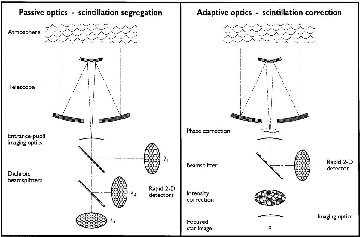
Fig. 10.— Telescope concepts for reducing scintillation "noise" in stellar observations. The passive system (left) incorporates a photometer that rapidly (≲10 ms) and with good spatial resolution (≲10 cm) measures the two‐dimensional brightness distribution over the entrance pupil, thus resolving the spatial, temporal and chromatic signatures of scintillation. The active system (right) incorporates second‐order adaptive optics, which measures the pupil illumination in real time and corrects the two‐dimensional intensity excursions across it (e.g., by imaging it through an adaptive two‐dimensional neutral‐density filter).
The passive system aims at recording as much as possible of the scintillation signature, so that it can be segregated and (at least partly) removed in the data reduction. The temporal and spatial scales over which scintillation must be recorded is set by the atmospheric "speckle pattern," independent of telescope size. As discussed in earlier papers, the spatial scale in this flying‐shadow pattern is given by the diffraction Fresnel‐zone rF = √λh, which, for λ = 500 nm and turbulence at 10 km, equals ≃7 cm. A wind speed of 10 m s−1 then implies a timescale of 7 ms. Thus, resolutions of ≲10 cm and ≲10 ms are called for (or, ideally, another factor of 3 or so better). These values will change somewhat between different geographical sites, and also between different nights and seasons.
An ideal passive system (Fig. 10, left) will not measure the focal‐plane image of a star, whose intensity is contaminated by atmospheric fluctuations. A measured change of the focal‐plane intensity cannot alone tell whether that change originated from scintillation effects. However, if scintillation is indeed the cause, its effects can be traced back to the pupil‐plane shadow‐pattern, whose properties then must obey the laws of atmospheric optics.
The photometry is performed on the "flying shadows" themselves, over the full area of the telescope entrance pupil. With (or without) some extra optics (depending on whether the telescope can be driven sufficiently far out of focus), an image of the telescope entrance pupil is formed onto a spatially resolving two‐dimensional detector, with rapid readout. To exploit the wavelength dependence of scintillation, these measurements should not be made in white light, but rather in different colors. In its simplest form, the detector could be a CCD running at video rates, although ultimately some photon‐counting device with higher time resolution would be desirable.
The scheme in Figure 10 uses two dichroic beam splitters in series to separate light of three wavelength regions onto three detectors whose pixel locations optically coincide on the entrance pupil. For a large telescope, the number of pixels required is substantial; while around 100 may suffice for a 1 m aperture, something like 10,000 would be required for a very large telescope. The readout must be made some 100 times a second, producing a respectable rate of data flow. Although lower resolutions also would carry parts of the information, such a system appears required to "fully" resolve the spatial, temporal, and chromatic signatures of scintillation. The system offers further potentials, e.g., the signal from the two‐dimensional detectors can be apodized in software, simulating an arbitrary apodized aperture and thus selectively depressing the most rapid scintillation components.
Satisfying all requirements of a high spatial and temporal (as well as some chromatic) resolution places an apparent‐magnitude limit on such a system. The white‐light flux on Earth from an mv = 0 star is on the order of 1012 photons m−2 s−1, i.e., at most ≃107 for each data point recorded in 10 ms over 0.01 m2, with λ/Δλ ≃3, assuming only modest instrumental losses. Meaningful scintillation estimates require perhaps 1000 photons per such data point, setting the limiting flux to perhaps 104 times fainter than mv = 0, i.e.,mv ≃10. A more detailed evaluation of the limiting magnitudes for high‐speed sensors recording over small subapertures is by Angel (1994).
7.3.1. Data Analysis for Segregating Scintillation
Using the data from such a system, the signatures of scintillation‐induced intensity fluctuations, ΔIscint, may be segregated from that of the true stellar intensity (unperturbed by atmospheric fluctuations),I*(λ). Scintillation has the effect of modifying the intensity (photon flux per unit area) falling onto the telescope to I(t,λ,x,y) = I*(λ) + ΔIscint(t,λ,x,y), where x and y are the spatial coordinates in the pupil plane. A detector system such as that in Figure 10 records this signal for different times, wavelengths, and spatial positions. To segregate I*(λ), a physical modeling of ΔIscint(t,λ,x,y) is required. The constraints in such modeling include (but need not be limited to) the following :
- 1.During a short observing period (10 s, say), the true stellar intensity can often be regarded as constant:I*(λ) = const, or else modeled as slowly varying with time.
- 2.I(t) = I*(λ) + ΔIscint(t,λ,x,y) must follow a lognormal distribution for all λ, x, and y (Paper I).
- 3.ΔIscint(x,y) must follow a relation such that the spatial power spectrum is consistent with that predicted from a Kolmogorov spectrum of turbulence (Paper I).
- 4.I(λ) must follow a relation such that the intensity variance σ2I at different wavelengths shows a λ−7/6 dependence (or perhaps somewhat weaker; Paper II).
- 5.I(t,λ) must follow a relation such that the timescales for σ2I at different wavelengths follow a √λ‐dependence (or perhaps somewhat weaker; Paper II).
- 6.I(λ,x,y) must follow a relation such that the spatial scales for ΔIscint(x,y) follow a √λ‐dependence (or perhaps somewhat weaker; Paper II).
- 7.I(t,λ,x,y) must show a behavior such that the velocity of the flying‐shadow pattern across the pupil is independent of λ (Paper II).
Using such types of constraints,I(t,λ,x,y) can be modeled in terms of its components I*(λ) and ΔIscint(t,λ,x,y), perhaps best by maximum likelihood fitting of the scintillation relations to observed data, taking the photon‐counting and detector noise into account. The amount of data produced in this scheme is considerable; already a short observation of 10 s, say, with a 2 m class telescope (300 spatial pixels, three wavelength channels, 10 ms time resolution) produces 106 intensity measurements of I(t,λ,x,y), from which I*(λ) is to be deduced. A full night's observation with a very large telescope would then produce more than 1010 measurements, a significant but not unreasonably large data volume by today's standards. Since the types of computations are repetitive in nature, and data can be handled sequentially in blocks of short observation periods, this appears well suited to automated data analysis schemes.
Unfortunately, it appears not straightforward to precisely quantify which components of this scheme can contribute what fraction of scintillation reduction (e.g., chromatic vs. temporal information; number of spatial channels vs. sampling rates). To obtain credible numbers appears to require numerical modeling and extensive simulations on a level that will make it a research project in its own right.
Although the physical concepts may appear simple, there are several degrees of freedom in parameterizing and modeling the flying‐shadow behavior. A higher spatial resolution across the telescope pupil on one hand improves the resolution of the flying shadows, but at the cost of making the imaging photometrically less precise due to increased photon noise. Similar trade‐offs go for the temporal and spectral resolutions. Utilizing chromatic cross‐correlations in scintillation may, away from zenith, permit a certain "early warning" since a disturbance in one color may appear earlier than that in another (Paper II). But how reliably can such a prediction be utilized? In some cases, perhaps apodization of the telescope aperture can be beneficial (by digitally weakening the signal from the aperture edges). Can this be further improved by adaptively changing the degree of apodization in real time, in response to, e.g., varying wind velocities?
Is there some additional information to be had from, e.g., imaging a pupil higher in the atmosphere, where there is less intensity variation? With a beam splitter, such a pupil could be incorporated (but at a cost in photon noise). If there is a known (average) height from which scintillation comes, that would simplify the modeling. The physical modeling might be improved if the actual (not idealized) properties of scintillation are better understood, e.g., the apparent deviation in its wavelength dependence from an idealized λ−7/6 law (Paper II).
While the scintillation amplitude of course is independent of stellar brightness, the quality of its segregation will depend on the stellar magnitude; the brighter the star, the less photon noise will affect the determination of scintillation parameters. Also, for measuring the wavelength dependence, a "white" star with adequate flux throughout the spectrum will be easier to measure than pronounced blue or red ones.
Perhaps one could apply some of the mathematical formalism developed for signal extraction in other fields of study. For example, considerable efforts have been invested in developing algorithms for optimally filtering photographic images against the noise in the emulsion (see, e.g., Katsaggelos 1991). When measured on a microphotometer, that noise usually appears approximately Gaussian in photographic density, corresponding to the logarithm of intensity. The mathematical problem of segregating (two‐dimensional) linear‐intensity images against a logarithmic grain noise in photography is thus of a similar character to segregating (one‐dimensional) stellar linear‐intensity variations versus time, against a background of logarithmic scintillation noise.
7.3.2. Simpler Reduction Schemes
Even at lower resolutions and slower sampling, some scintillation characteristics remain visible. Therefore, one can envision also simpler schemes that should be able to tangibly reduce scintillation noise, despite not fully resolving the flying‐shadow signatures.
Using only one temporal channel, one measures I(t) = I* + ΔIscint(t), i.e., as a conventional high‐speed photometer that records the intensity with ≲10 ms time resolution. The distribution of measured values, Ii, closely follows a lognormal distribution, and there will appear frequent "spikes" in the intensity record data, with amplitudes rather higher than expected, had the distribution been normally Gaussian (Paper I). Because these "spikes" may reach quite high values, they contribute a disproportionate fraction of the "noise" to a classically recorded photometric signal. If more spatial channels (resolving the entrance pupil) are available, the lognormal character of the signal will be better resolved.
Such time‐resolved data can be handled with different levels of sophistication. Even a temporal median filter would cut out events in the lognormal tail of the intensity distribution and the variance they contribute.
A better way would be to compute the logarithm of each intensity sample, and to average these logarithms, instead of the linear intensities. This is equivalent to taking the geometric mean, exp (〈ln Ii〉), of the time series (as opposed to the arithmetic mean,〈Ii〉, in classical photometry). In the limit of negligible photon noise, that is the quantity on which the mathematically optimum estimate of the average value of a lognormally distributed sample is based (see, e.g., Kendall & Stuart 1979, p. 74). However, the gains from this procedure alone will be modest. The variance of the estimated mean intensity will change by approximately a factor σ2I/[exp (σ2I - 1)], or ≃0.9 if we take σ2I = 0.2 as representative for fully resolved scintillation (Paper I). The geometric mean is smaller than the arithmetic one and requires a correction factor that in the lognormal case is equal to exp (σ2I/2). (The variance σ2I must therefore be estimated as part of the procedure.) In the limit of photon noise only, the counting statistics obey a Poisson distribution, and the optimum intensity estimate is simply the arithmetic mean; there are no gains from subdividing the measuring sequence.
For photometric light curves requiring high time resolution (i.e., not many orders of magnitude longer than scintillation timescales), it might perhaps be worthwhile to apodize the sampling time window, to depress noise components originating from occasional intensity "spikes" at the beginning or end of the sample time intervals.
Such schemes, involving high sampling rates, are related to efforts made elsewhere for reducing transparency (extinction) fluctuations for astronomical photometry. Those are caused by changes in the pressure, humidity and turbidity of the atmosphere blowing across the path between the observer and a star. Gains in the signal‐to‐noise ratio by factors ≃1.5 are reported when the data are initially recorded at high speed, and then suitably filtered, instead of merely pursuing an ordinary boxcar integration (Poretti & Zerbi 1993; Zhilyaev, Romanyuk, & Svyatogorov 1994).
7.3.3. Further Noise Reductions
The scheme of Figure 10 provides a further reduction of photometric noise. In ordinary photometers, a field (Fabry) lens is used to image the entrance pupil onto the detector. Its purpose is to avoid output variations caused by the focused stellar image moving across the surface of the nonuniform detector. Instead, the flying shadows in the entrance pupil are imaged onto the detector, which thus still experiences a variable illumination. Even if the shadow contrast is low, and their large numbers largely average out the fluctuations, this still does contribute to the apparent scintillation, and should also be eliminated. This is solved by spatially resolving the flying shadows, i.e., the atmospheric speckle pattern; there are no further spatial fluctuations inside each resolved speckle element.
To circumvent this noise source is, in principle, also feasible in more ordinary photometry, by bringing the light to an integrating cavity instead of imaging the pupil on the detector. However, such schemes are wasteful in terms of photons.
Once the atmospheric sources of intensity fluctuation can be contained, telescopic sources of analogous noise must also be tracked down. Telescope mechanics often imply tracking irregularities, vibrations, and other effects, which introduce a spatial modulation of the stellar image with high temporal frequency, possibly mimicking scintillation effects (Jenkins et al. 1996; Erm 1997; St‐Jacques et al. 1997).
Also, some use could be made of the experience gained in related laboratory experiments, where scintillation noise has been reduced by exploiting correlation between perturbations at different wavelengths (Kjelaas & Nordal 1982).
7.4. Active Systems: Second‐Order Adaptive Optics
Scintillation reduction is required not only for accurate photometry, but also for precise imaging beyond that permitted by ordinary ("first‐order") adaptive optics. Such systems correct the phase of the atmospherically distorted wavefront, in principle achieving plane‐wave imaging (see, e.g., Beckers 1993). The diffraction‐limited point‐spread function is then given by the Fourier transform of the illumination pattern across the telescope's entrance pupil. For uniform illumination, the ordinary Airy pattern results from a circular aperture (with spikes from the secondary‐mirror mount, etc.). However, irrespective of this phase correction, the pupil illumination has the character of bright and dark patches (flying shadows), and its Fourier transform contains additional structure. In particular, the flanks and wings of the image contain (time‐variable) illumination, making the detection of faint stellar companions difficult. To circumvent this requires "second‐order" adaptive optics, correcting not only the phase due to the angular tilt of the wavefront, but also amplitude effects from its curvature. Perhaps the most challenging application is to achieve direct imaging of planets around other stars with large ground‐based telescopes (KenKnight 1977).
Once ordinary ("first‐order") adaptive optics has achieved the phase corrections to high accuracy (and most of the light falls within the diffraction limit), second‐order effects from scintillation become dominant; the challenge is to reduce the residual and time‐variable "halo" around the central star. Simulations clearly show that phase corrections alone do not suffice, but also scintillation must be corrected. The imaging of extrasolar planets with large ground‐based telescopes appears to require scintillation corrections over subapertures of perhaps ø = 5 cm, sampled on timescales of perhaps 500 μs (Angel 1994; Stahl & Sandler 1995; Ryan 1996; Sandler et al. 1996; Sandler & Angel 1997).
Figure 10 (right) shows such an adaptive scheme for scintillation correction in real time. A uniform pupil illumination is achieved after imaging it through an adaptive two‐dimensional neutral‐density filter, whose transmission is the "inverse" of the flying‐shadow pattern.
Any actual system will involve many more complications than the sketch in Figure 10. For simplicity, what is sketched as an amplitude‐equalizing element is a multielement addressable filter, perhaps a liquid crystal, where response times of 10 ms appear practical (Bonaccini et al. 1990, 1991; Love, Fender, & Restaino 1995). It could also be a completely different optical arrangement, such as two phase‐correcting adaptive mirrors, each placed in one arm of a two‐arm interferometer. By modulating each accordingly, phase and/or amplitude would be shifted. When combining such units with first‐order adaptive optics (correcting the phase errors), a highly corrected focal‐plane image should result.
The flying‐shadow sensing device could well be different from a simple imager; one could instead measure the wavefront curvature by subtracting in‐focus and out‐focus images. The entrance pupil imaged in such signals appears very similar to flying‐shadow images (Takami & Kataza 1992; Ribak 1996). Whether artificial laser guide stars could be applied remains an open question.
Since the "guiding" is done on the same star that is being imaged, and the scheme contains no absolute flux reference, one should not expect the recorded flux to be of a high photometric stability. The purpose is to continuously remove the spatial intensity fluctuations across the entrance pupil in order to stop that pattern from being diffracted into the wings of the stellar image; this scheme is for imaging brown dwarfs and exoplanets close to their central stars, not for precise photometry.
This study is part of the high‐speed astrophysics program at Lund Observatory, supported by the Swedish Natural Science Research Council. The development of the QVANTOS instrument, used for the observations, was supported also by FRN, the Swedish Council for Planning and Coordination of Research. At Lund Observatory, we thank in particular research engineers H. O. Hagerbo, B. Nilsson, and T. Wiesel for their highly competent help with various electronic units. Laboratory studies of apodized apertures were made by J. Egonsson. The observations were made at the Research Station for Astrophysics on La Palma (Royal Swedish Academy of Sciences), which is part of the Observatorio del Roque de Los Muchachos of the Instituto de Astrofisica de Canarias. Their staff is thanked for valuable help during our several visits there. L. A. Marschall (Gettysburg College) kindly provided a bibliography on solar shadow‐band studies. Parts of the material for this paper were prepared by D. Dravins during a visitorship stay at European Southern Observatory in Garching.
Footnotes
- 1
See also http://www.hq.eso.org/.