804, 1998 September 10
© 1998. The American Astronomical Society. All rights reserved. Printed in U.S.A.

Simulations of Supernova Remnants in Diffuse Media and Their Application to the Lower Halo of the Milky Way. I. The High-Stage Ions

This paper reports on detailed, nonequilibrium hydrodynamic simulations of supernova remnants (SNRs) evolving in a warm, low-density, nonthermal pressure-dominated ambient medium (T = 10⁴ K, n = 0.01 cm^-3, P_nt = 1.8 × 10³ K cm^-3), with the goals of characterizing their structure and C⁺³, N⁺⁴, and O⁺⁵ content, emission, and line profiles and investigating the effects of supernova remnants in the lower Galactic halo. If undisturbed by external objects, these remnants have great longevity, surviving for 1.7 × 10⁷ yr. During the adiabatic phase, they contain large quantities of C⁺³, N⁺⁴, and O⁺⁵ in the hot gas behind their shock fronts. They emit brightly in the ultraviolet resonance lines and would appear edge brightened to observations of column density and emission. At the end of the adiabatic phase, each SNR develops a zone of cooling and recombining C⁺³, N⁺⁴, and O⁺⁵ in the transition region between the hot bubble and the cool shell. The resonance line luminosities plummet, and the edge brightening diminishes. As the remnants evolve, the interiors cool faster than the ions can recombine to their equilibrium levels. Thus, during most of the remnants' lifetimes the C⁺³ line widths are smaller than expected from collisional equilibrium, and after the remnants have completely cooled, some C⁺³ remains. The O⁺⁵, N⁺⁴, and C⁺³ distributions overlap incompletely. The O⁺⁵ ions are more plentiful in the warmer gas at smaller radii than are the N⁺⁴ or C⁺³ ions. As a result, after the shell forms the thermal pressure in the O⁺⁵-rich gas is at least twice as large as that in the C⁺³-rich gas. During most of its lifetime, the remnant's interior is less than 10⁶ K. Therefore, the fraction of area covered or volume filled by very hot SNR gas is much smaller than that filled by warm SNR gas. These simulations have been combined with the statistical distribution of isolated supernova progenitors in order to derive rough estimates of the appearance of the ensemble of isolated supernova remnants in the lower halo. The agreement between the simulation results and observational results in terms of average column density and spatial patchiness shows that much, if not all, of the high-latitude O⁺⁵, N⁺⁴, and C⁺³ between the local bubble and roughly a kiloparsec can be attributed to isolated SNRs in the lower halo. The simulations may also be of interest to studies of the external galaxies and the hypothesis that the Local Bubble is a single supernova remnant evolving in a low-density ambient medium.

Subject headings: Galaxy: halohydrodynamicsISM: generalmethods: numericalsupernova remnants

§1. INTRODUCTION

These hydrocode simulations show that an undisturbed supernova remnant (SNR) evolving in the Galactic halo contains warm gas and high-stage ions (C⁺³, N⁺⁴, and O⁺⁵) for approximately 1.7 × 10⁷ yr. The rate of isolated supernova explosions, integrated from ¹ z = 300 pc to infinity is about $\mathstrut{\frac {1}{6} }$ × 10⁵ yr kpc^-2 and is dominated by explosions of isolated, runaway O and B stars originating in the disk (Ferrière 1995). Combining the lifetime with the rate gives a rough estimate of the average occupancy at about 30 SNRs kpc^-2. Thus, there should be a significant number of supernova remnants in the halo. Most will be very old, although the younger ones are more recognizable. An example of a young halo SNR is the Kepler SNR, which is 600 pc off of the plane. ²

Because supernova remnants sculpt and supply energy, metals, and mass to the interstellar medium (ISM) and contain high-stage and X-ray line-emitting ions, the population in the halo is potentially important to the halo and may provide a significant key for interpreting the observations. Currently, some of the high-latitude observations are quite puzzling and the physical state of the halo is not well understood. The sources of the high latitude O⁺⁵, N⁺⁴, C⁺³, and X-ray emitting gas are not determined. Surely, multiple physical mechanisms are influencing the high-latitude gas. Estimating the contributions of each source type will be essential to the process of disentangling their effects. This paper discusses the supernova remnants' O⁺⁵, N⁺⁴, and C⁺³ spatial and temporal distributions, as well as their emission fluxes, line profiles, apparent thermal pressures, and scale heights, and compares with the observations, while Paper II pertains to the remnants' X-ray emission.

High-latitude observations of ultraviolet lines of N⁺⁴ and C⁺³ show that these ions have multikiloparsec scale heights (Sembach & Savage 1992; Savage et al. 1993). Shadowing by high-z clouds (Burrows & Mendenhall 1991; Snowden et al. 1991, 1994) and subtraction of the extragalactic component (Snowden & Pietsch 1995; Barber, Roberts, & Warwick 1996a; or Cui et al. 1996) indicates that soft X-ray emitting gas resides well above the Galactic plane.

Very energetic sources are required in order to ionize the atoms to these levels. For example, ionizing carbon to the C⁺³ level requires 47 eV, while ionizing metals to the levels needed for copious X-ray line radiation requires hundreds of electron volts. As a rough guide to the implied temperature, if the ions are in collisional equilibrium, then the temperatures are a couple hundred thousand for the high-stage ions to a couple million for the X-ray emitting gas. The spatial distributions are patchy and inconsistent with a potential ubiquitous layer of high-stage ions or X-ray emitting gas.

In various proposed explanations, highly ionized gas is either advected from the disk of the Galaxy into the halo or is ionized in situ in the halo. The remaining possibility is that the halo was heated when the galaxy formed; however, Spitzer (1956) found that gas originally at T 3 × 10⁶ K will have cooled since then.

In the fountain and chimney models, hot gas is advected from the plane into the halo, where it cools, loses buoyancy, and falls back toward the plane (Shapiro & Field 1976; Mac Low & McCray 1988). These models could produce large numbers of highly ionized atoms (Edgar & Chevalier 1986; Shapiro & Benjamin 1991) but are constrained by the assumption that the halo is deficient in material and pressure that would interfere with fountain activity and by the observed spatial and velocity distribution of cool (Danly 1989b) and hot gas.

In a somewhat different picture, superbubbles (hot, rarefied regions sculpted by the winds and supernova explosions of clustered O and B stars) originating in or near the plane of the galaxy expand into a tenuous halo. A recent analysis by Ferrière (1995) uses an approximate two-dimensional model for superbubble expansion into a stratified halo and for supernova remnant (SNR) evolution. Assuming that most of the halo volume is already hot and that the very hot interior of the superbubbles extend to the shock fronts, she shows that superbubbles can expand to great distances from the plane and survive for millions of years, effectively filling the halo and dwarfing the volume occupation of halo SNRs. At present, this model cannot be compared with high-energy observations because no ultraviolet resonance line or X-ray emission predictions exist.

In situ heating mechanisms include photoionization by O and B stars, planetary nebulae, diffuse hot gas, M stars, and the extragalactic flux (Bregman & Harrington 1986), the interaction between high-velocity clouds and the ambient gas (Hirth, Mebold, & Müller 1985), reconnection of displaced magnetic field lines (Raymond 1992), and SNR heating (Cioffi 1991; Shull & Slavin 1994). Shull & Slavin (1994) extrapolate from detailed calculations of isolated SNRs in the disk (Slavin & Cox 1993), finding several difficulties with the hypothesis that halo SNRs are producing all of the observed high-stage ions. Cioffi (1991) predicts that older halo SNRs are unrecognizable and dimmer than the extragalactic soft X-ray background. While confirming that result for old remnants, this work (in Paper II) finds that young halo SNRs are bright in the $\mathstrut{\frac {1}{4} }$ and $\mathstrut{\frac {3}{4} }$ keV bands.

This project is a careful reexamination of the effects of isolated supernova remnants evolving in the halo. It is particularly focused upon characterizing a halo SNR's appearance at various ages, learning whether halo SNRs should make a significant contribution to the quantities of UV resonance line-emitting ions (in particular, C⁺³, N⁺⁴, and O⁺⁵) in the halo, and determining whether remnants should be observable as individuals or as a collective population. The C⁺³, N⁺⁴, and O⁺⁵ results for a halo SNR evolving at z 1300 pc are presented in this paper, along with very rough estimates of the appearance of the population of halo SNRs. The X-ray properties and average volume occupation of these remnants are presented in later work, as are additional simulations used to better determine the effects of a population of SNRs in the lower halo.

Simulations of supernova remnants evolving in very diffuse surroundings were made by means of a detailed one-dimensional hydrodynamic computer code (similar to Cui & Cox's 1992 and Slavin & Cox's 1992, 1993 codes), employing thermal conduction, nonequilibrium ionization and recombination rates, and magnetic pressure. The (unmodeled) density gradient should have minimal effect because the hot bubble diameters are $\mathstrut{\frac {1}{3} }$ of the density scale height, and Maciejewski, Shelton, & Cox (1996) found that SNRs evolving in moderate density gradients are nearly spherical. The primary computer run used an explosion energy of 5 × 10⁵⁰ ergs, ambient density (n) of 0.01 atoms cm^-3, ambient temperature of 10⁴ K, and ambient nonthermal pressure (P_nt) equivalent to that of a 2.5 G effective magnetic field. Based on the H and H⁺ vertical distributions, the choice of n corresponds to z 1300 pc. A variety of ionization conditions appear in the halo gas, but whether the warm phase or the hot phase is more plentiful is not well determined. The choices of ambient thermal and nonthermal pressures used here apply if the halo is cool and dominated by nonthermal pressures (see Boulares & Cox 1990). Although the abundances of gas-phase metals in the halo are not well determined, the halo gas-phase abundances may be closer to solar than are those in the disk (Savage & Sembach 1996). Solar abundances are often used in SNR simulations of disk remnants and were used in these calculations.

In addition to their application to the halo, simulations of SNRs evolving in a low-density environment may also be of interest for other purposes, such as comparisons with observations of external, edge-on galaxies, providing a method of estimating the lower limit on the magnetic pressure, or evaluating the hypothesis that the Local Bubble is the hot bubble component of an SNR evolving in a low-density, nonthermal pressure-dominated region.

This paper is organized as follows: The halo observations are summarized in § 2. The ambient conditions used to set the input parameters for the simulation and the supernova progenitor statistics used to find the total contribution from an ensemble of remnants are discussed in § 3. The modeling algorithm is described in § 4. The simulated SNR's structure and evolution, as well as its high-stage ion content, morphology, thermal widths, and apparent thermal pressures are discussed in detail in § 5. Section 6 provides rough estimates of the absorption column densities, emission fluxes, and spatial distribution for the estimated population of isolated SNRs in the halo. Section 7 discusses what can be concluded as a result of these calculations, as well as comparisons with other models, applications to external galaxies and the local bubble, and the assumptions and approximations.

FOOTNOTES

¹ An inverted cone with a 40° half-angle and cut off below z = 300 pc has the same rate of 1 per 6 × 10⁵ yr.

² The Type Ia events account for about one-third of the supernova explosions above z 300 pc. SN 1006, which is 400800 pc above the plane (Long, Blair, & van den Bergh 1988), provides an example of this type of SNR residing in the halo.

§2. OBSERVATIONS

§2.1. C⁺³, N⁺⁴, and O⁺⁵

When very hot (T &gsim; 10⁶ K), highly ionized plasma abuts much cooler gas, a transition temperature zone should develop. In collisional equilibrium, the transition temperature gas (0.55 × 10⁵ K) is inhabited by lithium-like ions of carbon, nitrogen, and oxygen (C⁺³, N⁺⁴, and O⁺⁵; Shapiro & Moore 1976). Lithium-like carbon is not a unique tracer of hot regions because carbon can also be ionized to the C⁺³ level by 47 eV photons from starlight. Lithium-like nitrogen and oxygen, however, are good tracers because they require 77 and 114 eV photons, respectively, which are above the 54 eV He II edge present in O and B stars and produced in only modest quantities by the population of hydrogen-rich hot white dwarfs. Thus, O⁺⁵ and N⁺⁴ are thought to trace collisionally ionized gas, while C⁺³ is a more ambiguous ion.

These highly ionized species have strong ultraviolet resonance doublets and so will be called UV ions (or high-stage ions) in this paper. Most of the high stage ion data is in the form of absorption column densities seen in sight lines toward bright stars. The resonance transition lines for O⁺⁵ are at 1032 and 1038 Å, which are outside of the range examined by IUE and the GHRS but inside the range examined by Copernicus and the Orbiting and Retrievable Far and Extreme Ultraviolet Spectrometers (ORFEUS). The resonance lines of N⁺⁴ and C⁺³ are at 1239 and 1243 Å, and 1548 and 1551 Å, respectively, placing them within the IUE and GHRS ranges. As a result, the potential data sets of N⁺⁴ and C⁺³ observations are much larger than that of O⁺⁵, but the N⁺⁴ absorption column densities are often below the observability thresholds. A limited set of emission data is also available for C⁺³ and O⁺⁵.

§2.1.1. Variability

In looking from sight line to sight line, one finds considerable variation in the absorption column densities of the high-stage ions. Shelton & Cox (1994) statistically analyzed the O⁺⁵ data set, finding that the intersight-line variation was statistically significant: the data agree with a model in which these atoms are pooled into distinct regions within the interstellar medium (ISM), but not with one in which O⁺⁵ atoms are smoothly distributed. Although the available data set was dominated by disk sight lines, the trend appeared in both halo and disk subsets. Recently, several additional halo sight lines have been studied. Hurwitz & Bowyer (1996) and Hurwitz et al.'s (1995) ORFEUS data qualitatively show tremendous variation from sight line to sight line, with some directions having over 10¹⁴ O⁺⁵ atoms cm^-2 and others having less than 10¹³ O⁺⁵ atoms cm^-2.

The sets of C⁺³ and N⁺⁴ column density data also show variability. For examples, see Figure 8 of Savage et al. (1993), Figure 6 of Savage & Massa (1987), or Figures 4c and 4d of Savage et al. (1997). Savage et al. (1997) used a "patchiness parameter," _p, to model the intrinsic scatter in the data, finding that _p is about 0.30 dex for C⁺³ and about 0.24 dex for N⁺⁴. Interestingly, their Figure 4c shows that nine of the 17 sight lines below z = 1 kpc have C⁺³ column densities similar to or less than that attributable to the Local Bubble (assuming that the local bubble's contribution can be estimated from a Slavin & Cox 1992 supernova remnant, see below). None of the sight lines beyond z = 1 kpc have such low column densities. Thus, the distribution of C⁺³ below a kiloparsec has a moderate (50%) area coverage, while above 1 kpc it has a near unity area coverage. Furthermore, Savage et al. (1997) note that the sight lines with 2 < z < 5 kpc have larger ratios of C⁺³ to N⁺⁴ than either higher or lower sight lines, and Danly (1989a) shows that at around 1 kpc the velocity characteristics of her C⁺¹, Si⁺¹, and O⁺⁰ data set change markedly.

§2.1.2. Vertical Distribution and Average Column Densities

Although the C⁺³, N⁺⁴, and O⁺⁵ data show considerable sight line to sight line variation, it is still useful to infer a scale height for each by fitting to an exponential function. Before the Local Bubble was postulated, that equation was simply

where n(z) is the average volume density at height z, n₀ is the average midplane volume density, and h is the scale height. Integration provides the average projected (b = 90°) total column density between the midplane and extragalactic space, N_pr:

The hot Local Bubble is a potential complication because it may contribute ions to the line of sight totals and occupy space that could otherwise contain high-stage ions. For O⁺⁵, the contribution appears to be significant (1.6 × 10¹³ cm^-2; Shelton & Cox 1994). Before the local bubble was well understood, Jenkins (1978b) evaluated the O⁺⁵ scale height from the Copernicus data set, finding that h 300 pc. The number of halo sight lines in the Copernicus data set is rather small, so the scale height could not be determined well. The midplane volume density was thought to be n₀ = 2.8 × 10^-8 cm^-3, yielding N_pr 2.6 × 10¹³ O⁺⁵ cm^-2. Shelton & Cox (1994) subtracted the local bubble contribution and replotted the data. Their Figure 11 shows that scale heights between 300 and 3000 pc best fit the data. Adding new data from the ORFEUS detector but ignoring the Local Bubble contribution, Hurwitz & Bowyer (1996) arrived at a projected column density through the halo of 8 × 10¹³ O⁺⁵ cm^-2. An approximation to the new h can be found by means of N $\mathstrut{_{{\rm tot}}}$ =N $\mathstrut{_{{\rm lb}}}$ +n $\mathstrut{_{0}}$ he $\mathstrut{^{-z_{{\rm lb}}/h}}$ , where N_tot is the total column density on an idealized halo sight line, N_lb is the local bubble contribution, and z_lb is the height at which the sight line exits the Local Bubble. Taking N_tot to be Hurwitz & Bowyer's (1996) 8 × 10¹³ O⁺⁵ cm^-2, using n₀ from Shelton & Cox (1994), ³ and assuming that a typical z_lb for a halo sight line is about 100 pc × cos 45° yields a range of h's from 1100 to 1550 pc. Note that this is greater than the scale height found by Hurwitz & Bowyer (1996; 80 pc &lsim; h &lsim; 600 pc).

The N⁺⁴ estimates have varied: using IUE data, Sembach & Savage (1992) found that the N⁺⁴ projected column density is 2.5 × 10¹³ cm^-2. For an n₀ of 5.1 × 10^-9 N⁺⁴ cm^-3, h is 1.6 kpc. Later, Savage & Sembach (1994) and Sembach & Savage (1994) examined recent GHRS observations, finding that some of the N⁺⁴ values obtained from the IUE data were overestimates. In addition, the ORFEUS N⁺⁴ observations yielded only upper limits. As a result, Hurwitz & Bowyer's (1996) N⁺⁴ projected column density is only one-fifth of Sembach & Savage's (1992). Combining IUE and GHRS data, Savage et al. (1997) estimated the average midplane density at n₀ = (2.0 ± 0.5) × 10^-9 cm^-3, the exponential scale height at 3.9 ± 1.4 kpc, and n₀ × h at (2.5 ± 0.6) × 10¹³ cm^-2. The Local Bubble's contribution to the projected total N⁺⁴ column density can be estimated from Slavin & Cox's (1992 and 1993) supernova remnant models, ⁴ giving N_lb 2 × 10¹² cm^-2. This is less than a tenth of Sembach & Savage's (1992) or Savage et al.'s (1997) projected total and so probably has little effect on their determinations of n₀ or h.

Savage et al. (1997) found the exponential C⁺³ scale height to be 4.4 ± 0.6 kpc, the midplane density to be (9.2 ± 0.8) × 10^-9 cm^-3, and the projected total column density to be (1.2 ± 0.2) × 10¹⁴ cm^-2. If the Local Bubble column density is similar to that of a Slavin & Cox (1992) disk supernova remnant (2.5 × 10¹² cm^-2), then the Local Bubble contributes a negligibly small fraction of the projected total.

With an ionization potential of only 33 eV, Si⁺³ ions are even lower on the ionization scale than C⁺³. Savage et al. (1997) found the Si⁺³ exponential scale height to be 5.1 ± 0.7 kpc. They note a remarkable trend: h $\mathstrut{_{{\rm N}^{+4}}}$ < h $\mathstrut{_{{\rm C}^{+3}}}$ <h $\mathstrut{_{{\rm Si}^{+3}}}$ , yet the scale height of neutral hydrogen is smaller than all of these. The O⁺⁵ scale height extends the trend to h $\mathstrut{_{{\rm O}^{+5}}}$ <h $\mathstrut{_{{\rm N}^{+4}}}$ <h $\mathstrut{_{{\rm C}^{+3}}}$ <h $\mathstrut{_{{\rm Si}^{+3}}}$ . Regarding the reversal of the trend for H⁺⁰, it is conceivable that the z distribution is better described as a combination of a low scale height component and a higher scale height component. Lockman & Gehman (1991) found an H I scale height of 1 kpc, but Kalberla et al. (1997b) may have found a thick H I distribution with an exponential scale height of 4.4 kpc.

§2.1.3. Multiple Hosts or Differing Host Regimes? Absorption Profiles, Emission, and Thermal Pressure

The emerging picture of the high-stage ion distribution is further complicated by Savage, Sembach, & Cardelli's (1994) observation of multiple absorption profile types. The sight line toward HD 167756 (z = 850 pc) has a very broad C⁺³ velocity profile that correlates well with the N⁺⁴ profile. In addition, it has a couple of narrow C⁺³ features that correlate well with the Si⁺³ profile but that have little associated N⁺⁴. Savage et al. (1994) suggest that the broad and narrow features correspond to different types of hosts.

Assuming collisional processes, the electron density can be found from the emission and absorption data, using n_e = 4I/( &angl0; v &angr0; _eN), where I is the intensity, N is the column density, and &angl0; v &angr0; _e is the electron-impact excitation rate coefficient. Formally, the emission and absorption data should be for the same location on the sky, but the scarcity of data makes that impossible. Martin & Bowyer (1990) estimated that the n_e in the C⁺³ harboring regions is 0.01 cm^-3, giving a thermal pressure of P_th 1000k K cm^-3. In a more detailed analysis, Shull & Slavin (1994) calculated that 0.01 cm^-3 n_e 0.02 cm^-3 and 2200 K cm^-3 P_th/k 3700 K cm^-3. In contrast, Dixon et al. (1996) found that the electron density in O⁺⁵ harboring regions is 0.06 cm^-3, giving 22,000 K cm^-3 P_th/k 67,000 K cm^-3. Several possible circumstances may explain the vast difference in calculated thermal pressures: (1) the pointings are not coincident, (2) the formula breaks down if many of the ions result from photoionization, (3) the ion populations may be far from collisional equilibrium, affecting the excitation and de-excitation rates, (4) the O⁺⁵ may reside in hotter gas whose pressure is mostly thermal, and the C⁺³ may reside in cooler gas whose pressure is mostly nonthermal. This may be the case in the ancient halo SNRs simulated in this paper (see § 5.6).

§2.1.4. Estimating the Average Halo Flux

At this time, determining the average flux originating in the halo will be imprecise because the contribution from the local region (or other ubiquitous sources) is not known and because the observations do not provide averages for the halo (the current set of observations contains a large number of null detections of the O⁺⁵ emission and does not provide enough sampling to map the halo). The following estimates are provided in the context of these reservations. The interface between the hot Local Bubble and several cool clouds surrounding the Sun appears to provide very little flux. Slavin (1989) calculated the emission from a cloud that is evaporating via thermal conduction with a hotter environment. His result for the emission in the resonance doublet of O⁺⁵ is 254 photons cm^-2 s^-1 sr^-1, and his result for C⁺³ is weaker. The Local Bubble contribution is not known. Model estimates should depend on the stage of evolution, as well as the model parameters. If the Local Bubble is like a single SNR evolving in an n = 0.01 cm^-3, P_nt = 1800 K cm^-3 medium (see § 5.5), then the C⁺³ emission should range from about 1000 photons cm^-2 s^-1 sr^-1 before shell formation to about 100 photons cm^-2 s^-1 sr^-1 afterward, and the O⁺⁵ flux should range from about 5000 to about 500 photons cm^-2 s^-1 sr^-1. If the Local Bubble is more like an SNR in a denser ambient medium, then the emission during either developmental stage should be larger. For example, Slavin & Cox (1992) predict a C⁺³ flux of 750 photons cm^-2 s^-1 sr^-1 for a postshell-formation remnant (viewed from the interior) evolving in an n = 0.2 cm^-3 medium. A rough estimate for the flux from a preshell-formation remnant can be found by ratioing the above values.

In comparison, the average C⁺³ flux from Martin & Bowyer's (1990) high-latitude observations is 4700 photons cm^-2 s^-1 sr^-1. If the Local Bubble is like a preshell-formation SNR in a somewhat dense ISM, then it may provide all of this, but if it is like an SNR in a rarefied medium or like an old SNR, then it may provide little. Combining Dixon et al.'s (1996), Edelstein & Bowyer's (1993), and Korpela, Bowyer, & Edelstein's (1998) data gives an average O⁺⁵ flux that ranges from 8300 photons cm^-2 s^-1 sr^-1 if the null detections are taken as zero to 24,000 photons cm^-2 s^-1 sr^-1 if they are taken at the instrumental thresholds. ⁵ Considering the range in Local Bubble estimates, the local component could provide little to all of the observational average.

Because the nonlocal contributions are poorly constrained by the above approach, the following simple model may be comparatively fruitful. Suppose that the minimum value in the data set is for a field of view having only the local component, the maximum value is for a field of view having the local component and one halo SNR (in actuality, some of the bright fields intersect the North Polar Spur, which is thought to arise from events more energetic than a single supernova explosion, but that point will be ignored in this simple model), and in order to estimate the O⁺⁵ fluxes for which upper limits were found it is assumed that the pointings with null detections actually have only the local component. Thus, the estimated local contribution provides &lsim; 2200 C⁺³ photons cm^-2 s^-1 sr^-1 and &lsim; 10,000 O⁺⁵ photons cm^-2 s^-1 sr^-1 (for the C⁺³ case, the value is taken from a low-latitude pointing). The average high-latitude C⁺³ flux can be found without appealing to this model and is 4700 C⁺³ photons cm^-2 s^-1 sr^-1, while the average high-latitude O⁺⁵ flux found from this model is &gsim; 15,000 O⁺⁵ photons cm^-2 s^-1 sr^-1. In this simple model, the remaining fluxes are attributed to the halo: &gsim; 2500 C⁺³ photons cm^-2 s^-1 and &gsim; 5000 O⁺⁵ photons cm^-2 s^-1 sr^-1.

§2.2. X-Ray Observations

In summary, Snowden et al.'s (1998) analysis of the ROSAT PSPC R1 and R2 ( $\mathstrut{\frac {1}{4} }$ keV) data shows that the distant component (halo and extragalactic) of the northern sky provides about 4003000 × 10^-6 ROSAT $\mathstrut{\frac {1}{4} }$ keV counts s^-1 arcmin^-2. The northern sky contains some unusually bright features such as the Sco-Cen bubble, which contribute to this range. The distant component of the southern sky provides about 4001000 × 10^-6 ROSAT $\mathstrut{\frac {1}{4} }$ keV counts s^-1 arcmin^-2. (Note that these are not the observed count rates, rather they are the rates expected from the distant components before obscuration by the intervening material.) The extragalactic background contributes roughly 400 × 10^-6 ROSAT $\mathstrut{\frac {1}{4} }$ keV counts s^-1 arcmin^-2 of this (see Snowden & Pietsch 1995; Barber et al. 1996a; Cui et al. 1996). The spatial distribution has been shown to be "patchy" on a wide range of scales: 20° (Snowden et al. 1998), 1° (see Burrows & Mendenhall 1991), and 20 &arcmin; (Barber, Warwick, & Snowden 1996b). Assuming collisional equilibrium of the ions, the temperature of the distant component is thought to be about 1 × 10⁶ K, with ±20% variation depending on direction (Snowden et al. 1998), with some groups preferring slightly higher temperatures (2 × 10⁶ K; Wang & McCray 1993; Kerp 1994). Breitschwerdt & Schmutzler's (1994) nonequilibrium models and the X-ray results presented in Paper II, however, show that the X-ray producing gas need not be hot. Highly ionized warm gas also produces X-rays.

FOOTNOTES

³ While a fully self-consistent method would use a range of n₀'s found for a range of h's and N_lb's and then check for consistency, a full range is not available. Shelton & Cox (1994) found n₀'s and likely N_lb's for h = 300 and 3000 pc. The scale heights found in this work are, reassuringly, between that range.

⁴ Fig. 7 in their 1992 paper provides the average column density from all lines of sight through the remnant. The average column density for the sight line from the interior to the outside should be about one-fourth of that.

⁵ Some of the instrumental thresholds are much higher than some of the detections, artificially inflating the average.

§3. MODEL PARAMETERS FOUND FROM THE OBSERVATIONS

§3.1. Ambient Conditions

§3.1.1. Gas Density

The vertical distributions of neutral and ionized hydrogen are taken from Ferrière (1995), who calculated them from Dickey & Lockman's (1990) compilation of 21 cm and H data and from Reynolds (1991) free electron distribution.

The primary supernova remnant simulation presented in this paper uses an ambient atomic density of n = 0.01 cm^-3. Additional simulations use n = 0.05, 0.02, and 0.005 cm^-3. The hydrogen to helium ratio is assumed to be 10 to 1, so the heights corresponding to these mass densities are z $\mathstrut{_{{(}n=0.05\,{\rm cm}^{-3}{)}}}$ =480 pc, z $\mathstrut{_{{(}n=0.02\,{\rm cm}^{-3}{)}}}$ =850 pc, z $\mathstrut{_{{(}n=0.01\,{\rm cm}^{-3}{)}}}$ =1300 pc, and z $\mathstrut{_{{(}n=0.005\,{\rm cm}^{-3}{)}}}$ =1830 pc. The hydrocode also takes the environmental gas to be fully ionized, as may be the case if it is preionized by the SNR. Thus the ratio of particles to atoms is taken as 23/11. If the ambient environment is not preionized, then the ambient particle density will be slightly less than assumed. It is more important to calculate z's that correctly correlate to the mass density (which plays an important role in determining the swept-up mass) than to use z's that precisely correlate to the thermal pressure (which plays only a minor role in determining the total pressure). Nonetheless, the interested reader will find that at heights of z = 350, 690, 1170, and 1760 pc, the densities of particles in a fully ionized medium are the same as those in a partially ionized medium having densities of atoms of n = 0.05, 0.02, 0.01, and 0.005 cm^-3, respectively.

§3.1.2. Pressures

The thermal conditions in the halo vary greatly and are poorly determined. For example, assuming that the ions are in collisional equilibrium, the large $\mathstrut{\frac {1}{4} }$ keV emission measures (Snowden et al. 1998) suggest that patchily distributed, 10⁶ K gas resides somewhere in the halo and occupies z 1 kpc, while the large scale heights of Si⁺³ (Savage et al. 1997) and H I (Kalberla et al. 1997b) suggest that warm and cool gas extend well into the halo. Furthermore, some cold gas resides in the halo, patchily distributed over much of the sky. It is possible that any of the components could fill significant fractions of the lower halo (that with 300 pc &lsim; z &lsim; 1000 pc). Opinions vary greatly as to which set of n and T best describes this region, with the chosen set being a reasonable point for beginning a computational exploration of parameter space. For the simulations presented in this paper, the temperature of the ambient medium is taken to correspond to the Reynolds layer, T = 10⁴ K. At this temperature, the ionized gas with a hydrogen to helium ratio of 10 to 1 and an atom density of n = 0.01 cm^-3 has a thermal pressure of 2.9 × 10^-14 ergs cm^-3 or 210 K cm^-3. The turbulent pressure in the halo is thought to be small (Ferrière 1995) and is not explicitly included in these simulations.

The ambient nonthermal pressures (magnetic and cosmic ray) are also poorly known, but models and observations provide some clues. Boulares & Cox (1990) created a set of hydrostatic models of the galaxy, including magnetic tension and various forms of the gravitational potential. In their array of models, the lowest value of the magnetic pressure found at z = 1200 pc is 7.5 × 10^-13 ergs cm^-3. This corresponds to an rms magnetic field of B = 4.3 G, from P_B = B²/8. Kalberla, Pietz, & Kerp's (1997a) hydrostatic model yields a similar field strength (3.9 G). The observational evidence also suggests that the magnetic pressure may be large. Kazès, Troland, & Crutcher's (1991) measurement of H I Zeeman splitting in the high-velocity cloud HVC 132+23-212 shows that the magnetic field in the cloud is 11.4 ± 2.4 G. They point out that this value is similar to that for normal Galactic H I clouds and surmise that there is no evidence of compression or enhancement of the magnetic field in the high-velocity cloud. This cloud is at the end of complex A (Lillienthal, Meyerdierks, & de Boer 1990), whose height is z 4 kpc (Wakker et al. 1996).

The lowest value for the cosmic-ray pressure at z = 1200 pc from the Boulares & Cox (1990) models of the Galaxy is 4 × 10^-14 ergs cm^-3, while the values from their preferred models are 5 × 10^-13 ergs cm^-3. Because the generally accepted nonthermal pressure is lower than these values and because preliminary simulations using 4 times the following nonthermal pressure yielded similar but slightly smaller remnants, having comparable high-stage ion column densities during their youths, this paper concentrates on runs made with P_nt = 2.5 × 10^-13 ergs cm^-3 (1800 K cm^-3). Although the choice of P_nt makes only a small effect on the total numbers of high-stage ions, increasing P_nt noticeably increases the high-stage ion and the X-ray emissions. See Paper II. The physical picture drawn from these choices of thermal and nonthermal pressures is of a cool, nonthermal pressure-dominated plasma. This picture differs from the hot halo sometimes envisioned, and so the model is but one contribution to the set of potential simulations necessary to cover the entire range of possible ambient conditions.

§3.1.3. Metallicities

The gas-phase metal abundances are generally greater in the halo than in the disk, but less than in the Sun (Savage & Sembach 1996). Savage & Sembach (1996) show that the gas phase abundance of sulfur in the halo is approximately solar, the abundance of silicon is slightly less, and the abundances of magnesium, manganese, chromium, and iron are approximately one-third solar. It is thought that dust grains have been disrupted to a further extent in the halo gas than in the disk gas, which explains the higher gas-phase abundances, especially of particular elements. As is common in SNR simulation projects (Slavin & Cox 1992, 1993), solar abundances are assumed. In this case those of Grevesse & Anders (1989) are used. The metal-rich supernova ejecta complicate this simple picture. Some of the metal atoms may be quickly bound up in dust grains. Those remaining in the gas phase should have a limited influence on the SNR emission structure because their number is soon diluted by the number of swept-up metal atoms.

§3.2. Supernova Parameters

The Type Ia supernova explosion rates are taken from Ferrière (1995). The rate for Type Ia supernovae is thought to be about once per 445 yr, while the combined rates for Types Ib and II supernovae is thought to be about once every 52 yr. Using these values, Ferrière (1995) found the volumetric rate of Type Ia supernovae at our galactocentric radius to be

Type Ib and Type II supernovae are thought to occur in massive stars. Estimating that 60% of Type Ib and II supernovae are clustered while 40% are isolated runaways, using a total galactic rate for Type II supernovae, and calculating that the runaways have a scale height of about 266 pc, Ferrière (1995) found the volumetric rate at the solar circle for isolated Type Ib and II supernovae to be

The remaining 60% of Type Ib and II progenitors are thought to have much smaller velocities and so go supernova predominately in or very near to the plane. Finding a greater density of massive stars at the solar radius than that of Ferrière (1995), McKee & Williams (1997) derived twice the rate per unit area of high-mass progenitors. Combining their rate with Ferrière's (1995) remaining calculations and assuming that this result and Ferrière's (1995) original volumetric rate bracket the true rate yields

A Type Ia supernova can arise from a white dwarf in a binary system with a companion that overflows its Roche lobe. Before becoming a white dwarf, the star sheds several solar masses. These outflows modify the local ambient medium but are not included in the modeling. Isolated Type Ib and II progenitors tend to be somewhat massive and emit winds that also modify the local ambient medium. In addition, they can leave behind pulsars that emit energy. Neither effect is explicitly modeled in this project. This is easily justified because the structure of the ISM very near to the progenitor should be eroded by the SNR, particularly after the SNR has greatly expanded and evolved. In addition, there is a precedent for modeling the presupernova stellar wind energy by slightly increasing the input supernova energy (Ferrière 1995). The kinetic energy produced by a supernova explosion is not precisely known; it is generally taken to be about 0.51.0 × 10⁵¹ ergs. This paper uses a total initial energy of E₀ = 0.5 × 10⁵¹ ergs.

§4. MODELING THE EVOLUTION

§4.1. Hydrocode

The evolution is modeled using a spherically symmetric, explicit, Lagrangian scheme. Finite difference forms of the hydrodynamic and ion evolution equations are used (Richtmyer & Morton 1967). The important physical equations are the conservation of mass, momentum, and energy (eqs. [8], [9], and [10]), as well as the generation of entropy owing to the shock passage, the transfer of energy due to thermal conduction, and the loss of energy due to nonequilibrium radiative cooling. The conservation equations are

and

where is the mass density, t is time, r is the distance from the origin to the center of the parcel, v is the parcel's velocity, P_th is the thermal pressure, P_nt is the nonthermal pressure, P_v is the viscous pressure, is the adiabat, F_tc is the thermal conduction flux, and &epsis; is the radiative emissivity.

Each time step is much shorter than the time required for any parcel's energy, volume, or position to change substantially. Equations (8), (9), and (10) were integrated using the single step, explicit, finite difference method for Lagrangian hydrodynamics (see Richtmeyer & Morton 1967). Approximately 5 × 10⁵ time steps are used to simulate 2 × 10⁷ years of evolution.

Equal electron and ion temperatures are assumed throughout. The hydrogen and helium in the SNR and ambient medium are assumed to be fully ionized. Using n for the density of nuclei gives P_th 23/11nkT. Magnetic and cosmic-ray pressures contribute a nonthermal pressure term, P_nt, which is modeled in a simplified fashion via an effective tangential magnetic field, B_eff. Thus, P $\mathstrut{_{{\rm nt}}}$ =B $\mathstrut{^{2}_{{\rm eff}}}$ /8, and owing to flux freezing, B_eff n. An artificial viscous pressure term is used to generate the entropy contributed by the shock where the pressure gradients are too large for reversible flow equations to apply. See Richtmyer & Morton (1967) for greater detail.

Thermal conduction occurs when fast-moving particles from a hot zone transfer energy to slower moving particles in an adjacent cooler zone. If the collisional mean free path is small compared with the length scale of the temperature gradient, then the thermal conduction flux is described by the classical equation: F_cl = -T^5/2(T/r). In steep temperature gradients, the energy transport rate saturates at about the speed of sound and the saturated form is used: F_sat = 4.5nkT(kT/m)^1/2. Various interpolations between the classical and saturated forms appear in the literature. In this hydrocode, the interpolation is taken as

The classical thermal conduction flux parameter from Spitzer (1956) is used, so = 6 × 10^-7 ergs cm^-1 s^-1 K^-3.5, while the saturation flux coefficient used is $\mathstrut{\frac {2}{3} }$ of that used in Cowie & McKee (1977). Magnetic effects on the conduction rate have been ignored: the interested reader is referred to discussions in Slavin & Cox (1992) and Shelton et al. (1998).

Above T 10⁷ K, bremsstrahlung is the dominant cooling mechanism. From 10⁴ to 10⁷ K, most of the emissivity is due to line emission from collisionally excited ions. In order to keep track of the ionization levels and cooling at each time step in the simulation, the ionization state is integrated along with the physical variables using Edgar tables (see Gaetz, Edgar, & Chevalier 1988) for the ionization and recombination rate coefficients and the Raymond & Smith (1977, 1993 private communication) integration routine. The cooling coefficient is then found from the ion concentrations convolved with Edgar tables of ion specific rates. These tables are limited to temperatures between 10⁴ and 10⁸ K. If the temperature is above 10⁸ K then the bremsstrahlung equation is used to calculate the emissivity and the Edgar ionization and recombination rate table values at T = 10⁸ K are used to update the ionization levels.

In order to retain accuracy, yet reduce CPU usage, the time-dependent ionization, recombination, and cooling coefficients are used only for those parcels that have ever been as hot as 5 × 10⁴ K and a cooling curve is used for the remaining parcels. The cooling curve was made from a nonequilibrium simulation of shock-heated, isobaric, radiating gas. The 5 × 10⁴ K cutoff criterion is so conservative that any parcel that could ever produce C⁺³, N⁺⁴, O⁺⁵, or X-rays would have its cooling calculated from the Edgar tables during the entire lifetime of the SNR.

§4.2. Caveats

The starting configuration in the simulation does not include the mass or metals in the ejecta and expresses the explosion energy as thermal energy. This approximation should have minimal effect on an ancient remnant because the mass and metals are soon diluted by swept-up gas and the appropriate fraction of the thermal energy is quickly converted into kinetic energy.

The hydrocode assumes spherical symmetry. As a result, it cannot explicitly model multidimensional instabilities, mixing, or deformations. The Vishniac instability is thought to act on the thin shell just after its formation, but is not thought to break up the shell (Ferrière 1995). The simulations do not explicitly model the multidimensional mixing between the ambient medium and the outermost SNR material after the shock front has merged with the ambient medium. As shown in § 5, however, this process does not hasten the hot bubble's life. Observations of SNRs show that they generally have asymmetries and filaments. If such structures exist for much of the remnant's lifetime, they could increase the volume of gas residing between hot and cool regions. This gas performs much of the cooling of the SNR, and so increasing its volume would increase the emission fluxes and concentrations of O⁺⁵, N⁺⁴, and C⁺³ but would decrease the remnant's lifetime.

The halo has a density gradient, but it is weak, and according to Maciejewski et al. (1996) SNRs react to weak density gradients by shifting their centers toward the lower density region while remaining nearly spherical in shape.

Magnetic tension is not included. Based on Slavin & Cox's (1992) examination, magnetic tension should reduce the maximum size of the hot bubble by a few percent and cause the bubble to begin its contraction slightly early. Ferrière, Mac Low, & Zweibel (1991) and Ferrière & Zweibel (1991) demonstrated the presence of a relatively uniform environmental magnetic field leads to magnetic tension in the cool shell, which causes it to elongate, become asymmetric, and have nonradial motions. The shell becomes thinner where the ambient magnetic field is directed perpendicular to the shock front and thicker where the magnetic field is parallel to the shock. Because the thinned region is a very small fraction of the surface area, the asymmetries should cause minimal changes in the total number of high-stage ions in the remnant during the stages modeled by Ferrière & Zweibel (1991) (before the shock slows to a magnetohydrodynamic wave). Tomisaka's (1990) calculations extend to later times, showing that the shell continues to grow asymmetrically on both its outer surface and its inner boundary with the hot bubble. It is conceivable that the thinnest parts of the shell may become important after the shock slows, primarily because the thinned shell may be less effective in protecting the hot cavity from premature decay due to mixing and cooling via thermal conduction with the ambient gas. These effects cannot be modeled with the one-dimensional hydrocode.

The hydrocode does not model differential galactic rotation, upward movements due to buoyancy, collisions with other objects, or the effects of an inhomogeneous ambient medium. The hydrocode does not prevent radiative cooling in regions of high viscous pressure, although this seems to have had little effect, and it does not calculate photoionization effects.

§5. STRUCTURE AND EVOLUTION OF A HALO REMNANT

§5.1. Evolution Overview

Immediately following a supernova explosion, the supersonic ejected material shock heats and sweeps up the ambient material into a dense, outwardly moving rim of material. ⁶ The outermost part of the rim, the shock front, expands at supersonic speeds and so shock heats and sweeps up its neighboring ambient gas. As the SNR expands, the shock weakens. As a result, it heats the encountered gas to lesser and lesser temperatures. Eventually the dense gas slightly interior to the shock front meets the conditions for rapid cooling, and this gas evolves into a cool shell. Beyond the cool shell lies a thin zone of warm, very recently shock-heated gas that will soon radiate away most of its thermal energy and so will become part of the cool shell. Interior to the cool shell lies the hot bubble.

With the specified ambient conditions and explosion energy, the cool shell forms between 2.5 and 5 × 10⁵ yr. Afterward, the remnant (defined as the shock region, cool shell, and hot bubble) expands faster than the hot bubble, stretching the cool shell. In addition, the warm gas on either surface of the cool shell radiates quickly and joins the shell. As a result, the cool shell becomes extremely "thick" (large r) and relatively diffuse, contrary to the "thin shell approximation."

The remnant continues to expand until the shock has slowed to the magnetohydrodynamic wave speed of the ambient medium, whereupon it is thought to merge with the ambient medium. This occurs around 8 × 10⁵ yr, when the radius is 170 pc and the hot bubble radius is 120 pc. After the ambient medium and shock front merge, the ambient medium mixes and exchanges heat with the newly exposed material just interior to the destroyed shock front. Both effects proceed at approximately the speed of sound. In the standard semianalytic scenario the hot bubble is separated from the shock front by only a "thin shell" and so is immediately exposed to the ambient medium. In that case, mixing and thermal conduction lower the plasma's temperature to the point where, if it were in collisional equilibrium, it would enter the rapid cooling regime. As a result, the hot bubble would diminish in size at about the rate of the sound speed. (This is well described in Ferrière 1995). In the hydrocode simulations, however, the hot bubble is separated from the shock front by a very thick zone of already cooled material and so is not affected by the shock front's demise. In the simulation, the hot bubble slowly cools by radiative cooling and by conducting heat to the cooler gas on its periphery. The cooler periphery meets the conditions for fast cooling and so radiates more efficiently than the interior. Because thermal conduction to neighboring, more efficiently radiating material is also the primary destruction process in the standard semianalytic scenario, the hydrodynamically simulated remnant is no longer lived than would be expected if mixing with the ambient medium were to be more explicitly modeled.

§5.2. Structure

§5.2.1. Temperature

The simulated halo SNR is much hotter at a given radius, forms a shell much later, and lives much longer than a simulated SNR evolving in the disk (Slavin & Cox 1992). Figure 1 shows the kinetic temperature of the gas as a function of radius from the center of the remnant for 24 epochs ranging in ages from 1.0 × 10⁴ to 1.8 × 10⁷ yr. At 10⁴ yr, the interior temperature is 2 × 10⁷ K. It is uniform throughout the remnant due to thermal conduction. As the remnant adiabatically expands the interior temperature drops, such that by 10⁵ yr it is 3 × 10⁶ K.

Fig. 1

The shock front also weakens as it expands, causing the shock to heat the gas to lesser and lesser temperatures. By 10⁵ yr, the cooling rate, which depends strongly on the density, temperature, and ionization state, becomes significantly greater for the denser, 2 × 10⁶ K gas on the periphery than for the rarer, 3 × 10⁶ K gas in the center. This causes the temperature profile to develop a rounded shape, which is clearly evident by 10⁵ yr. Such gas will develop into a nascent cool shell between 10⁵ and 2.5 × 10⁵ yr. By 5 × 10⁵ yr, some parcels have cooled to the temperature of the ambient medium and completed the development.

After the shell forms, three mechanisms compete with each other to control the hot bubble's expansion. The thermal pressure within the hot bubble is less than the nonthermal pressure in the cool shell, the hot bubble gas still has inertia, and the gas at the bubble's periphery rapidly cools and defects from the hot bubble to the cool shell. As a result, the hot bubble continues to grow, but at a slower rate, until around 2 × 10⁶ yr. Its maximum radius is 140 pc. Henceforth, the bubble slowly collapses. The interior temperature drops from about 10⁶ to 6 × 10⁵ K during its last 1.5 × 10⁶ yr of growth, and from 6 × 10⁵ to 3 × 10⁵ K during its first 10⁷ yr of collapse. Over the subsequent few million years, the temperature drops rapidly so that by 1.7 × 10⁷ yr the SNR has completely cooled.

When the SNR wave reached the edge of the simulation grid, a fraction of the energy reflected off of the boundary, causing an artificial returning wave. This is the source of the nonphysical structure between 220 and 400 pc in Figure 1. In addition, at late times, the temperature profile shows some structure within the cool shell. This is an artifact of the code and does not affect the O⁺⁵, N⁺⁴, or C⁺³ results.

§5.2.2. Density

Figure 2 depicts the density as a function of radius from the center for 1.0 × 10⁴ to 1.8 × 10⁷ yr. For the first 10⁵ yr, the SNR has two major zones, a diffuse interior and a dense rim just behind the shock front. By 2.5 × 10⁵ yr, the material behind the shock has cooled to nearly the ambient temperature and so is beginning to form a third zone, the cool shell. This is clearly evident by 5 × 10⁵ yr. The shock front expands significantly faster than the hot bubble, causing the shell to grow in width and diminish in compression.

Fig. 2

The compression factor reaches its maximum as the gas behind the shock front begins to cool significantly (2.5 × 10⁵ yr). The compression slowly decreases from then on, with the shell density approaching that of the ambient medium within a couple million years. The small compressions imply that observational techniques based solely on observing dense regions will have difficulty identifying the shells of the older SNRs.

The density within the supernova remnant bubble is never less than 10^-3 cm^-3. If thermal conduction had not been included, the central density would be less. Thermal conduction moves heat from the center outward, leveling the temperature distribution. In order to maintain a relatively constant pressure distribution in the central regions, the density profile must flatten in the interior. Physically, this occurs via a slowing of the expansion in the center of the remnant. Note also that the enhanced densities plotted at large radii and late times are an artifact of the code and not associated with the SNR.

§5.2.3. Pressure

During the early stages, the SNR's expansion is driven by the large thermal pressure (P_th) of the interior. The nonthermal pressure contributes little. As the shell material cools and compresses, however, its thermal pressure drops and its nonthermal pressure rises. Thus, after the shell forms, the high pressure in the shock front is due to nonthermal pressure (see Fig. 3).

Fig. 3

All the while, the hot bubble is adiabatically, radiatively, and conductively cooling, causing its thermal pressure to drop. By 1 × 10⁶ yr, P_th in the interior is actually less than the total pressure of the ambient medium. Over the next several million years the hot bubble collapses, and so its thermal pressure increases slightly. By 10⁷ yr, P_th begins to decrease again. Note that the incoming wave seen at 220, 280, 340, and 405 pc on the last pressure plot is an artifact.

§5.2.4. Velocity

The gas velocities are presented in Figure 4. Early on, the velocity structures (velocity as a function of radius) are typical of the blast wave stage. The velocity structure begins to change noticeably between 0.5 and 1 × 10⁶ yr (between the last curve in Fig. 4a and the first curve in Fig. 4b). By 3 × 10⁶ yr, the cooling and contraction of the hot bubble causes the gas near the periphery of the hot bubble to begin to recede faster than any other part of the SNR. This characteristic persists throughout the SNR's life and becomes more noticeable as time progresses.

Fig. 4

§5.3. C⁺³, N⁺⁴, and O⁺⁵

Figures 5, 6, and 7 depict the fraction of oxygen, nitrogen, and carbon found in the lithium-like states (O⁺⁵, N⁺⁴, and C⁺³) as a function of radius and at various epochs. At 1.0 × 10⁴ yr, these ions can be found at nearly all radii within the SNR (Figs. 5a, 6a, and 7a). The very hot, but tenuous (3 × 10⁷ K and 0.003 cm^-3) interior is very slow to ionize and so still contains O⁺⁵, N⁺⁴, and C⁺³ and lower ions at 10,000 yr. It is more difficult to ionize oxygen to O⁺⁵ than to ionize nitrogen and carbon to N⁺⁴ and C⁺³. Thus, ionization to the O⁺⁵ level lags behind that of the other high-stage ions; half of the carbon in the center has reached the C⁺³ level, but only a quarter of the oxygen has reached the O⁺⁵ level. Just behind the shock, there is a slim spike of UV ions. We are glimpsing the atoms as they quickly transit the lithium-like ionization states.

Fig. 5

Fig. 6

Fig. 7

By 2.5 × 10⁴ yr (see Figs. 5b, 6b, and 7b) the gas in the interior has ionized beyond the O⁺⁵, N⁺⁴, and C⁺³ states. The ions are found only in a slim region just interior to the shock front, where the substantially underionized ⁷ 10⁷ K atoms are racing through the ionization states. This pattern continues through 10⁵ yr. By 2.5 × 10⁵ yr, however, the shock is too weak to heat the gas to more than 10⁵ K and the high-stage ions are no longer found near the shock front. Instead, they lie at the periphery of the hot bubble. In this case, the rapidly cooling gas is overionized ⁸ and recombining through the O⁺⁵, N⁺⁴, and C⁺³ states.

Because the oxygen recombines through the O⁺⁵ state sooner than the carbon recombines through the C⁺³ state, most of the O⁺⁵ resides at slightly smaller radii than most of the C⁺³. This effect develops before 2.5 × 10⁵ yr but is more obvious in succeeding epochs. At 10⁷ yr (Figs. 5c, 6c, and 7c), the C⁺³ and O⁺⁵ are almost entirely noncoincident. One ramification is that some sight lines through the SNR will traverse only the C⁺³-rich regions, while others will encounter much more O⁺⁵ than C⁺³. Thus, as seen in the observational data, there will be great variation in the C⁺³/O⁺⁵ ratio. Another ramification is that the O⁺⁵ lies in 2 × 10⁵ K and hotter gas while the C⁺³ lies in 10⁴ to 2 × 10⁵ K gas. The line profiles for the ions will differ, as will the thermal pressures calculated from the emission fluxes and absorption column densities (see § 5.6).

The distribution patterns of the high-stage ions at 10⁷ yrs (Figs. 5c, 6c, and 7c) are fairly representative of those from 1 to 12 × 10⁶ yr, except for shifts in the location of the bubble edge. The C⁺³ lies in the warm gas at the bubble's periphery and in the cool gas just beyond the bubble. The O⁺⁵ lies in the warm gas at the bubble's edge but also in the center of the remnant.

By 1.2 × 10⁷ yr, the temperature in the center of the SNR is only 3 × 10⁵ K. In the subsequent epochs, the temperature drops and the density increases rapidly. The ions recombine through the O⁺⁵ state so that O⁺⁵ and even lower ions can be found in the center of the SNR. As in previous epochs, the C⁺³ distribution extends to greater radii than that of O⁺⁵ and some of the C⁺³ resides in the recently cooled gas beyond the edge of the hot bubble. This is illustrated by Figures 5d, 6d, and 7d for the remnant at 1.5 × 10⁷ yr of age. By 1.7 × 10⁷ yr, the entire SNR has cooled to the ambient temperature. The number of O⁺⁵ ions has dropped to 10^-4 of its value at 1.5 × 10⁷ yr and a million years later the O⁺⁵ is gone entirely. The C⁺³ lingers longer. It does not disappear entirely until 1.9 × 10⁷ yr.

Considering the entire lifetime of the remnant, we see that the UV ion-rich gas is underionized for less than 2.5 × 10⁵ yr or less than 1.5% of the SNR's life and is overionized for the remainder. The gas cools (sometimes significantly) before it recombines. For example, C⁺³ can be found in the cool shell just beyond the edge of the hot bubble and exists out to a radius of 25 pc at 18 × 10⁶ yr, in spite of the fact that the entire remnant has cooled to 10⁴ K a million years earlier.

§5.4. Absorption Column Densities and Velocity Profiles

§5.4.1. Column Densities

The C⁺³, N⁺⁴, and O⁺⁵ column densities were calculated by integrating the abundances and densities along the line of sight. The C⁺³, N⁺⁴, and O⁺⁵ column densities as a function of impact parameter and epoch are presented in Figures 8, 9, and 10, while the average column densities and total numbers of ions in the supernova remnant are presented in Table 1.

Fig. 8

Fig. 9

Fig. 10

At 10⁴ yr, the O⁺⁵ is distributed throughout the SNR, but is most plentiful just behind the shock front. The O⁺⁵ column density is fairly constant with impact parameter at this epoch (see Fig. 8a). For the next hundred thousand years, the O⁺⁵ is confined to a thin region just behind the shock, and as a result, the SNR is very edge brightened in O⁺⁵. By 2.5 × 10⁵ yr a cool shell has begun to form, and now the O⁺⁵ is slightly less well confined to a region of cooling, recombining gas on the periphery of the hot bubble. The SNR still appears to be edge brightened (see Fig. 8b). As time progresses, gas further interior to the bubble's periphery recombines to the O⁺⁵ state. As a result, the SNR appears less edge brightened in O⁺⁵. By 10⁷ yr, the fraction of oxygen in the O⁺⁵ state is approximately constant throughout the hot bubble, but the SNR still appears slightly edge brightened because the density of atoms is larger near the periphery (see Fig. 8c). Henceforth, the column density near the edge begins to drop (see Fig. 8d).

The column densities vary less with time than do the emission fluxes presented in § 5.5. For most epochs and impact parameters, if the O⁺⁵ column density were fully observed (see the following discussion on line profiles), it would be of the same order of magnitude as the observed column densities (8 × 10¹³ cm^-2 for the halo and disk [Hurwitz & Bowyer 1996] minus 2 × 10¹³ cm^-2 for the local bubble [Shelton & Cox 1994]).

The N⁺⁴ and C⁺³ column density plots are similar to those for O⁺⁵, with the following exceptions. From 2.5 × 10⁵ yr onward, the C⁺³ exists out to greater radii than does the N⁺⁴, and the N⁺⁴ exists out to greater radii than does the O⁺⁵. This trend strengthens with time, such that the O⁺⁵ disappears long before the N⁺⁴ or the C⁺³. After the formation of the shell the C⁺³ profile is more edge brightened than the others. As a result of these effects, the ratios of C⁺³ to N⁺⁴ to O⁺⁵ are strongly dependent on impact parameter and SNR age. In addition, by 4 × 10⁶ yr the C⁺³ profiles develop a double peak (which can also be found in the N⁺⁴ profiles at later times), which is correlated to the double peak in the ion fraction plots. Perhaps most importantly, a single simulated SNR provides much smaller C⁺³ and N⁺⁴ column densities than expected from high-latitude observations, while it provides nearly as much O⁺⁵ as expected from observations. This contrast is evaluated in § 6.

§5.4.2. Velocity Profiles

The widths of the velocity profiles affect the ease with which the column densities can be seen via absorption measurements and provide diagnostics for comparisons with observations. Figure 11 depicts the velocity profiles for lines of sight through the center of the SNR at 10⁴, 2.5 × 10⁵, and 10⁷ yr representing the three phases of the SNRs life.

Fig. 11

For the first 10⁵ yr, the hot bubble extends to the shock front. The resulting velocity profiles are multipeaked because the ions in the interior of the remnant have almost zero bulk velocity, while the ions near the shock front have very large bulk velocities. The peaks are hundreds of km s^-1 wide, largely due to thermal broadening associated with the very hot plasma. If absorption measurements were taken for the SNR at this epoch, determining the full column densities could be quite challenging. The low- and high-velocity peaks merge, giving the false appearance of discrete absorption features combined with a continuum. The high-velocity peaks (both the positive velocity peak, which is illustrated in the figure, and the negative velocity peak, which is not depicted) and most of the zero velocity curve are well beyond the range generally observed with the Copernicus instrument responsible for most of the existing O⁺⁵ column density data ⁹ although they are within the ORFEUS range. ¹⁰ In addition, the profiles are so broad that they may be difficult to identify.

By 2.5 × 10⁵ yr, the high-stage ions reside at and near the boundary between the hot bubble and the cool shell. Because the hot bubble is still expanding rapidly, the peaks of the ion velocity profiles are between 90 and 100 km s^-1 (see Fig. 11b). The C⁺³ resides at greater radii than the others and so has a faster velocity centroid and smaller velocity dispersion. The full width at half-maximum for the O⁺⁵ is 28 km s^-1. Applying the Maxwell Boltzmann distribution function [FWHM = 2(2kT ln 2/mass)^1/2] gives a temperature ¹¹ of 2.73.5 × 10⁵ K for the O⁺⁵, with the range being due to the finite velocity resolution in Figure 11. The N⁺⁴ distribution corresponds to a temperature of 1.72.4 × 10⁵ K and the C⁺³ distribution gives a temperature of 5.18.4 × 10⁴ K. The determined temperature for C⁺³ is less than the temperatures at which the ions are most abundant if collisional ionization equilibrium is assumed. In addition, the observations of the velocity profiles provide a way to corroborate the earlier claim that the C⁺³ resides predominantly in the tepid gas of the nascent cool shell while the O⁺⁵ and N⁺⁴ lie in the hot gas on the outskirts of the bubble.

The simulated SNR bubble spends roughly 80% of its lifetime (from 3 to 18 million years) slowly contracting. The 10⁷ yr epoch provides a typical example. As we saw in Figure 5 the O⁺⁵ resides everywhere in the interior of the remnant. So, although the remnant is collapsing at about 5 km s^-1, the O⁺⁵ velocity profile in Figure 11c appears as a single peak centered at 0 km s^-1. The temperature calculated from the FWHM is 3.03.2 × 10⁵ K, approximately that of the bubble interior. The FWHM of the N⁺⁴ profile implies a temperature of 1.21.3 × 10⁵ K. The C⁺³, however, is confined to the periphery of the hot bubble, and so its profile has discrete peaks. The half-width implies a temperature of only 2.02.4 × 10⁴ K, consistent with Figures 1, 2, and 7. The temperature is much lower than C⁺³'s equilibrium temperature of 1.1 × 10⁵ K because the gas has cooled faster than it recombined.

§5.4.3. Comparison with Expectations from Simulated SNRs in Moderate Density Media

Slavin & Cox (1993) parameterized the high-stage ion content of simulated supernova remnants having n = 0.11.0 cm^-3. This paper describes a simulation made with a similar hydrodynamic code, but at a significantly lower ambient density. Thus, this simulation can be used to determine to what extent the parameterization for simulated disk SNRs can be extended to include halo supernova remnants.

Using equation (8) from Slavin & Cox (1993), with E₅₁ = 0.5, n₀ = 0.01 cm^-3, and $\mathstrut{{\ucpmathaccent{P}{"707E}}}$ $\mathstrut{_{04}}$ =0.201 yields the following estimates for the time- and space-integrated ion contents (the dosages, D's): D(O⁺⁵) 1.6 × 10⁶² O⁺⁵ yr, D(N⁺⁴) 9.4 × 10⁶⁰ N⁺⁴ yr, and D(C⁺³) 2.4 × 10⁶¹ C⁺³ yr. For comparison, the dosages from the halo SNR are D(O⁺⁵) = 2.4 × 10⁶² O⁺⁵ yr, D(N⁺⁴) = 2.2 × 10⁶¹ N⁺⁴ yr, and D(C⁺³) = 4.9 × 10⁶¹ C⁺³ yr. Thus, the halo SNR contains 1.5, 2.3, and 2.0 times that expected from the parameterization of simulated disk remnants, indicating that the high-stage ion contents of the halo SNRs depend even more strongly on the ambient conditions than those in the disk SNRs.

§5.5. Emission

The emission was calculated from the densities, temperatures, and nonequilibrium ionic abundances using the Raymond & Smith spectral code (1977, 1993 private communication). The luminosities and average photon fluxes emitted by the entire SNR in the O⁺⁵ resonance doublet at 1032 and 1038 Å, the N⁺⁴ resonance doublet at 1239 and 1243 Å, and the C⁺³ resonance doublet at 1548 and 1551 Å are listed in Table 2. The photon flux as a function of impact parameter and epoch is presented in Figures 12, 13, and 14.

Fig. 12

Fig. 13

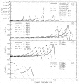Fig. 14

The brightest phase in the SNR's lifetime is before the shell forms. During this period, the rim of hot, dense material just behind the shock front meets the conditions for high emission: high temperatures, relatively large densities, and significant fractions of its O, N, and C in the O⁺⁵, N⁺⁴, and C⁺³ states. The rim produces nearly all of the flux, making the SNR appear edge brightened.

The luminosities begin to drop when the cool shell begins to form. The O⁺⁵ and N⁺⁴ emission patterns remain strongly edge brightened until 5 × 10⁵ yr, when the recombining gas within the interior begins to contain a significant fraction of these ions. In contrast, the C⁺³ distribution remains strongly confined and its emission pattern retains its edge brightened appearance until the last few million years

As with the absorption column densities, the C⁺³ emission extends to slightly greater impact parameters than the N⁺⁴ emission, which extends to greater impact parameters than the O⁺⁵ emission. Also, before the shell forms, the ions have large bulk and thermal velocities that spread their velocity distributions.

§5.6. Disparity in the Apparent Thermal Pressures

Because the C⁺³ and O⁺⁵-rich regions are generally offset from one another, these ions experience different ratios of thermal to magnetic pressure. The effect is obvious after the cool shell forms, when some of the C⁺³ resides in the cool shell while the O⁺⁵ resides in the warm gas on the periphery of the hot bubble. These plasmas have comparable total pressures, but the cool shell has a lower thermal pressure and larger nonthermal pressure (magnetic and cosmic-ray pressures) than the hot bubble. To demonstrate this point, the electron densities, temperatures, thermal and nonthermal pressures in the C⁺³-rich and the O⁺⁵-rich regions at 2.5 × 10⁵, and 10⁷ yr are reported in Table 3. For comparison, the table also lists the electron densities found via the standard method used with observational data (this method uses the ratio of the absorption column density to the emission flux), the collisional equilibrium temperature for the O⁺⁵-rich and the C⁺³-rich plasmas, and the resulting estimated thermal pressures.

Not only does the table verify the disparity between the simulated thermal pressures in the C⁺³-rich and the O⁺⁵-rich regions, but it also shows that the disparity would be obvious even if the thermal pressures were calculated using the observational techniques applied to the hydrocode predictions.

This comparison shows that it is possible that some ¹² of the disparity in the thermal pressures found from the observations could be because the C⁺³-rich gas has a lower temperature, lower thermal pressure, and higher magnetic pressure than the O⁺⁵-rich gas. If halo SNRs provide much of the observed high-stage ion column densities and emission fluxes in the direction chosen, or if the high-stage ion bearing gas is comparable to SNR gas in having noncoincident UV-ion distributions but similar total pressures in these regions, then the nonthermal pressure in the C⁺³-rich gas can be estimated from: P_nt &gsim; P_th(O⁺⁵ gas) - P_th(C⁺³ gas). In some scenarios, this value may provide a lower limit on the nonthermal pressure in the ambient medium.

§5.7. Observability of a Single Halo SNR

During most of its lifetime, a single simulated halo SNR has high-stage ion column densities of several times 10¹³ O⁺⁵ cm^-2, several times 10¹² N⁺⁴ cm^-2, and about 1 × 10¹³ C⁺³ cm^-2. Thus, if real halo SNRs are like the one simulated, then a single halo SNR intersected by a highlatitude sight line would provide a significant fraction of the observed O⁺⁵. While a single halo SNR would provide only meager fractions of the total N⁺⁴ or C⁺³ column density on a high-z sight line, it would provide significant fractions of the N⁺⁴ and C⁺³ column densities on a z &lsim; 1300 pc sight line (see Fig. 4 of Savage et al. 1997). Among the ramifications of these comparisons is the possibility of testing for halo SNRs by examining high-latitude O⁺⁵ data and high-latitude, z &lsim; 1300 pc N⁺⁴ and C⁺³ data.

FOOTNOTES

⁶ In discussions of very young supernova remnants, this accumulation of hot, dense, swept-up gas is often called a shell, but in discussions of long-term SNR evolution (such as this) the word shell is reserved for the dense gas only after it has cooled.

⁷ The atoms are less ionized than would be expected if the plasma were in collisional equilibrium. In collisional equilibrium, C⁺³ is most prevalent at 1.1 × 10⁵ K, N⁺⁴ is most prevalent at 1.9 × 10⁵ K, and O⁺⁵ is most prevalent at 3.2 × 10⁵ K (Shapiro & Moore 1976).

⁸ The atoms are more highly ionized than would be expected if the plasma were in collisional equilibrium.

⁹ The Copernicus detectors were programmed to scan 0.65 Å wide regions centered on the 1032 and 1038 Å O⁺⁵ lines (Jenkins 1978a). This equates to a velocity coverage of -95 to +95 km s^-1

¹⁰ The Berkeley Spectrometer on the ORFEUS telescope had simultaneous coverage of the 3901170 Å range (Hurwitz & Bowyer 1996).

¹¹ Strictly speaking, this method yields an upper limit on the true temperature because variation in the bulk velocity along the line of sight can contribute to the velocity dispersion. In this particular case, only a small fraction of the spread is due to dispersion in the bulk velocity.

¹² The apparent thermal pressure found from C⁺³ measurements can also be affected by the presence of photoionized C⁺³ along the line of sight. If these ions are cool, they emit little resonance line flux. As a result, they contribute little to the emission measure but contribute significantly to the total column density.

§6. THE ENSEMBLE OF REMNANTS

Estimates of the average column densities, emission fluxes, and areas covered by the population of isolated SNRs in the halo can be found by combining the above results with the distributions of isolated supernova progenitors. This method is approximate because nearer to the plane, the progenitor rates are larger but the SNRs are smaller and shorter lived. For example, the explosion rate in the region between z = 100 (roughly the average height of the local bubble) and 300 pc is equal to that between z = 300 pc and infinity, but the time-integrated numbers of high-stage ions in the 100 pc z 300 pc remnants are only about 1/10 as large. In order to avoid large overestimates of the average column densities and emission fluxes produced by the ensemble of remnants the following results use z = 300 pc as a lower bound, and in order to provide even better estimates of these quantities a later paper reports on SNRs simulated for a range of heights.

§6.1. Absorption Column Densities

Integrating equations (5) and (7) with respect to z between z = 300 pc and infinity produces an isolated SN rate per unit area of 1.72.9 × 10^-6 kpc^-2 yr^-1. Integrating the UV-ion content with respect to time gives 4.9 × 10⁶¹ C⁺³ yr, 2.2 × 10⁶¹ N⁺⁴ yr, and 2.4 × 10⁶² O⁺⁵ yr. The products of these numbers are the time- and space-averaged column densities of the population of SNRs in the lower halo: 0.891.5 × 10¹³ C⁺³ cm^-2, 4.06.8 × 10¹² N⁺⁴ cm^-2, and 4.37.3 × 10¹³ O⁺⁵ cm^-2.

§6.2. Emission

The time-integrated luminosities from a single halo SNR are 1.4 × 10⁴⁹ ergs for the O⁺⁵ doublet, 1.9 × 10⁴⁸ ergs for the N⁺⁴ doublet, and 4.5 × 10⁴⁸ ergs for the C⁺³ doublet. Combining these values with the integrated supernova rate and converting the units yields time- and space-averaged fluxes of: 340580 O⁺⁵ photons cm^-2 s^-1 sr^-1, 5594 N⁺⁴ photons cm^-2 s^-1 sr^-1, and 170290 C⁺³ photons cm^-2 s^-1 sr^-1. Increasing P_nt can significantly increase the time-integrated flux.

§6.3. Spatial Distribution

Simulations can be used to estimate the fraction of the sky that is covered by isolated halo supernova remnants. The lower z supernova remnants will be more plentiful, smaller, and shorter lived than the higher z remnants. Therefore, the fraction of area covered must be calculated at a series of heights and the results summed. Ideally, each of the simulations should be run using nonequilibrium ionization rates and the area should be found from the greatest extent of the high-stage ions, but that is CPU expensive. For this calculation, the simulations were run using a cooling curve and the area is found from the greatest extent of the T 20,100 K gas ¹³ For a thin slab of thickness z at height z, the fraction of the area covered by halo SNRs is the supernova rate for the slab multiplied by the time integral of the area covered by a single SNR.

Simulations were run for n = 0.05, 0.02, 0.01, and 0.005 cm^-3 (§ 3.1) these densities correspond to heights z = 480, 850, 1300, and 1830 pc. The slab boundaries are drawn halfway between each of these z's. Table 4 shows the supernova rate integrated with height for each slab, the time-integrated area covered by a single SNR, and the resulting fraction of area covered by SNRs in each slab.

Because two SNRs may overlap, Poisson statistics are then employed to calculate the fraction of sky covered by one or more isolated halo SNRs. The isolated SNRs above z = 290 pc should cover about 25%45% of the high-latitude sky, while, taking the 160 pc z 290 pc remnants to have the same physical sizes as those between 290 and 660 pc, the isolated remnants above z = 160 pc should cover about 40%58% of the sky.

The type of measurement that is best suited for comparison with the area coverage is absorption line studies of the high-stage ions, especially those of O⁺⁵. The C⁺³ data provide a less direct comparison because some of the detected ions may be due to photoionization. The emission data are less useful because each remnant is bright for only a small fraction of its lifetime, after which its fluxes are below the instrumental thresholds. Similarly, the X-ray emission is only bright for a small fraction of the remnants' lifetimes.

The relatively large area coverage could mislead one into believing that the fraction of volume filled by hot gas is also large. It is not, primarily because during much of the SNR's lifetime, the bubble is tepid (for our purposes, 2 × 10⁴ K &lsim; T &lsim; 8 × 10⁵ K) and contains high-stage ions, but is not hot (>8 × 10⁵ K) and produces little X-ray emission. The fraction of area covered by hot gas in SNRs above 160 pc is only 3%, and the volume filled is less than 2%.

The distribution of hypothesized halo SNRs across the sky will cause large scale variation. Edge brightening will cause medium scale variation, and structure within the SNR (owing to turbulence or inhomogeneities in the ambient medium) will cause smaller scale variation. In addition, because the O⁺⁵, N⁺⁴, and C⁺³ are sometimes concentrated in different parts of the remnant, individual sight lines through a remnant may detect a range of O⁺⁵ to C⁺³ column density ratios, as well as differing line widths.

FOOTNOTES

¹³ The simulations were tested for sensitivity to this threshold. Raising the temperature threshold by a factor of 10 lowered the area integral of the n = 0.02 cm^-3 SNR by only 20%.

§7. DISCUSSION

§7.1. Comparing Simulations with Observations of the Lower Halo: Conclusions

On average, a b = ±90° sight line through the ensemble of simulated SNRs above z 300 pc would encounter a column density of 4.37.3 × 10¹³ O⁺⁵ cm^-2, or 70%110% of the observationally determined column density after the local bubble has been subtracted (6.4 × 10¹³ O⁺⁵ cm^-2), leaving little need or room for other O⁺⁵ producing phenomena.

The halo's O⁺⁵ column densities vary greatly, with some sight lines having no O⁺⁵ beyond that expected from the local region (for example, Leo in the Jenkins 1978a data set). This indicates that the sources are distributed in a patchy fashion and do not cover the entire sky. The results of combining the simulations with the SNR progenitor distributions shows that the high-stage ions in halo SNRs should cover about 25%45% of the sky above z 300 pc and about 40%58% of the sky above 160 pc. Thus, the model for halo SNRs also has a patchy distribution, with less than complete sky coverage.

It is not possible to precisely calculate the observational average O⁺⁵ flux originating in the halo for comparison with the simulation average found for the ensemble of halo SNRs. It is possible to compare maxima, however. The maximum O⁺⁵ flux found from the predictions is 3.6 × 10⁴ photons cm^-2 s^-1 sr^-1. This lies in the middle of the detected range, with the caveat that some of the detected flux may be due to larger bubbles such as that associated with the North Polar Spur.

The set of C⁺³ observations give a much greater average absorption column density through the halo (1.2 × 10¹⁴ cm^-2) than that predicted for the ensemble of halo SNRs (0.891.5 × 10¹³ cm^-2), while the observational reports of the average N⁺⁴ column density vary, with the estimated average column density from the population of halo SNRs (4.06.8 × 10¹² cm^-2) lying near the low end of the observationally determined range.

Figures 4c and 4d of Savage et al. (1997) show that slightly more than half of the z 1300 pc sight lines have C⁺³ and N⁺⁴ column densities that are comparable to those expected from a single simulated z = 1300 pc SNR, while the remaining sight lines have only the column density that can be attributed to the Local Bubble. Considering that the area covered by z > 160 pc SNRs is estimated at approximately 40%58%, the likelihood that a random high-latitude sight line would intersect an SNR is similar to the fraction of z 1300 pc sight lines having column densities like those in the halo SNRs. These agreements suggest that the halo SNRs may be responsible for much of the C⁺³ and N⁺⁴ found below z = 1300 pc.

As in the observations of O⁺⁵ emission, the predicted time- and space-averaged C⁺³ flux is less than the instrumental thresholds, but the peak predicted flux is similar to those observed. In contrast with the O⁺⁵ data, the C⁺³ data of Martin & Bowyer (1990) have no high-latitude null detections. In addition, half of their pointings are far from the North Polar Spur.

The observations show that the N⁺⁴ velocity profiles are sometimes wider than those for C⁺³ on the same line of sight, as do the simulations. The observational data show great variation in the ratio of C⁺³ to O⁺⁵ on a given sight line (see Spitzer 1996), as do the simulations. Like the observational results, the halo SNRs have greater thermal pressures in their O⁺⁵-rich regions than in their C⁺³-rich regions, although photoionization to the C⁺³ level can also cause some disparity.

As discussed in great detail in Paper II, the time- and space-averaged $\mathstrut{\frac {1}{4} }$ keV X-ray count rate attributable to halo SNRs depends on the ambient nonthermal pressure and the explosion energy. For P_nt = 7200 K cm^-3 and E₀ = 1 × 10⁵¹ ergs, the predicted population of halo SNRs can explain the surface brightness of the southern hemisphere's halo. X-ray bright young halo SNRs should cover a small fraction of the sky, while older, dimmer remnants should cover about half the high-latitude sky.

The picture emerging from these points is that if the assumed simulation parameters adequately describe the halo and if the simulations reasonably represent actual supernova remnants in the halo, then the distribution of halo SNRs are important components of the halo below about 1300 pc, but that an additional source for C⁺³ and possibly N⁺⁴ is required above about 1300 pc.

§7.2. Comparisons with Other Work on Halo SNRs

In order to evaluate the possibility that halo SNRs could be responsible for all of the high-stage ions, Shull & Slavin (1994) applied several criteria to predictions from extrapolations of comparable simulations done with larger n (Slavin & Cox 1993). They pointed out that the high C⁺³ scale height (4.9 kpc from Savage et al. 1993) is not consistent with the low N⁺⁴ scale height (1.6 kpc) reported by Sembach & Savage (1992). Since that work, additional N⁺⁴ data have been reported such that Savage et al. (1997) now put the N⁺⁴ scale height around 3.9 kpc. Shull & Slavin (1994) also point out difficulties in obtaining a large flux in the C⁺³ resonance lines from the same gas that produces an average column density of around 10¹⁴ cm^-2. The simulations presented in this paper agree in general with their conclusions while contributing to our picture of the lower halo and providing useful detail: unless the progenitor scale height or ambient conditions at several kiloparsecs differ greatly from those expected or unless the very high z SNRs are very different than expected, the total high-z quantity of C⁺³ ions in the population of halo SNRs will be less than that observed in the halo, but the C⁺³, N⁺⁴, and O⁺⁵ observed below about 1300 pc can be attributed to supernova remnants in the lower halo. While an SNR is young, it can produce a large ratio of flux to column density, but the flux decreases much earlier than the column density. The time-averaged ratio is rather small. Note that the local regions' contribution to the total observed flux needs to be subtracted from the measurements before they are compared with the estimates and that the local contribution to the emission is poorly constrained. The simulations presented in this paper provide about twice as many high-stage ions as predicted by the extrapolation (eq. [9]) used in Shull and Slavin.

Ferrière (1995) used a numerical code to simulate SNRs in the halo. Our codes and ambient temperatures differ, but our conclusions that the isolated SNRs fill a tiny fraction of the halo concur.

§7.3. Implications for the Local Bubble

Models for the local bubble span a wide range, from single supernova explosions in a low-density medium (i.e., Cox & Anderson 1982; Arnaud, Rothenflug, & Rocchia 1984; Edgar 1986) to multiple explosions in a high-density cloud (Breitschwerdt & Schmutzler 1994). The results of this simulation project apply best to the first model.

Several observational constraints apply.

1. Using the Copernicus data set (Jenkins 1978b), Shelton & Cox (1994) found that the typical contribution from the local region is about 1.6 × 10¹³ O⁺⁵ cm^-2.

2. The velocity profiles of the subset of sight lines that are thought to have only the local component do not indicate fast expansion or exceptionally hot gas.

3. The instrument scanned near the O⁺⁵ resonance lines ± 100 km s^-1, so very fast or wide velocity components would not be found from the data.

4. Recently, Snowden et al. (1998) separated the distant and local components of the $\mathstrut{\frac {1}{4} }$ keV flux, finding that the local bubble provides between 250 and 820 × 10^-6 counts s^-1 arcmin^-2 with a color temperature (found from the ratio of the count rates in the ROSAT PSPC R1 and R2 bands) around 10⁶ K.

5. The bubble is not isotropic and has an average apparent radius of about 50100 pc.

6. Little edge brightening is apparent in the local bubble. In addition, the local bubble of X-ray emitting material does not appear to extend to the edge of the local cavity in several locations.

A priori we do not know the age of the SNR. If it is in the adiabatic evolutionary stage, then the simulated X-ray emission is bright enough and of the appropriate color temperature for agreement with the observational results, but the simulations show edge brightening while the existing observations do not, and the simulated O⁺⁵ velocities and thermal widths would be too large to explain the Copernicus observations (Jenkins 1978a; Shelton & Cox 1994). It is conceivable that the O⁺⁵ constraint could be satisfied if the evaporating local cloud (Slavin 1989) provides the slower, narrower O⁺⁵ components that were observed.

Another possibility is that the SNR is somewhat older. Once the cool shell forms, the O⁺⁵ resides only in the hot bubble, which is moving much slower than the shock front. For this reason and because the line widths are relatively narrow, the O⁺⁵ should be more easily detected by the Copernicus observations. In this case, producing too much O⁺⁵ becomes a concern, but for a significant range of SNR ages and local cloud parameters, the combined predicted column density falls within the expected range. Once the shell forms, the $\mathstrut{\frac {1}{4} }$ keV X-ray emission ceases to be very edge brightened, but also diminishes by an order of magnitude. The X-ray productivity of older SNRs depends critically on the ambient nonthermal pressure, allowing the possibility that an ancient SNR in a diffuse environment having a higher nonthermal pressure than was used for this paper may simultaneously explain the Local Bubble's X-ray brightness and its slow O⁺⁵. Thus, an additional source of X-rays is required. Perhaps the SNR ejecta should be considered because it could increase the X-ray emission from the interior of the remnant. Thus, the inclusion of the ejecta could assist this model for the local bubble on two fronts: it increases the total count rate and does not contribute to edge brightening. This scenario may be constrained, however, by abundance determinations from high-resolution spectra. In one of their tests, Sanders et al. (1997) fit the Diffuse X-Ray Spectrometer data with a collisional equilibrium, single temperature, variable abundance model, finding that the best fit had very low abundances of silicon, sulfur, and iron, but point out that speculation regarding the nature of those low abundances will probably be premature until more exhaustive modeling of their data has been completed.

§7.4. Applications to External Galaxies

Some external galaxies appear to have bright H and X-ray emission originating at least a couple of kiloparsecs from their disks and at large galactocentric radii. Two examples are NGC 891 and NGC 4631 (Dettmar 1990; Pildis, Bregman, & Schombert 1994; Bregman & Pildis 1994; and Wang et al. 1995). Often the emission is attributed to outflows from the disk. For example, Dettmar (1990) points out that the most extended and brightest high-z H region in NGC 891 is located above the largest H II regions in the disk, concluding that the H is associated with the disk activities. It is also conceivable that isolated events in the halo may be playing a role, as would be suggested by the spatial distribution of $\mathstrut{\frac {1}{4} }$ keV emission in NGC 4631 (see Fig. 1 of Wang et al. 1995).

For comparison with the fluxes and high-stage ion column densities in external galaxies, the simulation results have been parameterized for a rate of one supernova explosion per year per cubic kiloparsec. The ROSAT PSPC R1, R2, and R4 band count rates are 9, 6, and 0.3 counts s^-1 arcmin^-2 per kiloparsec of depth of the emitting region, respectively. The emission flux in the C⁺³, N⁺⁴, and O⁺⁵ resonance lines are 10^-3, 5 × 10^-4, and 4 × 10^-3 ergs cm^-2 sr^-1 s^-1 per kiloparsec of depth of the emitting region, respectively. In terms of photons, these numbers are 10⁸, 3 × 10⁷, and 2 × 10⁸ photons cm^-2 s^-1 sr^-1 per kiloparsec of depth of the emitting region. The absorption column densities in the C⁺³, N⁺⁴, and O⁺⁵ doublets are 5 × 10¹⁸, 2 × 10¹⁸, 2.5 × 10¹⁹ cm^-2, respectively. These are averages over the entire SNR's lifetime and so correspond to samplings large enough to contain many SNRs. If the examined region has few SNRs, with the young bright ones contributing the vast majority of the emission flux, then the more appropriate numbers for comparison would be the maximum fluxes for a single SNR presented in §§ 5.4 and 5.5 and in Paper II.

§7.5. Assumptions and Approximations

Because it is impractical to model every physical effect in detail, some physical effects are modeled in a detailed and CPU intensive manner at the expense of others. This code carefully models nonequilibrium ionization and recombination and simulates the entire lifetime of the remnant, but at the expense of not being able to follow movements in three dimensions. Thus, modeling turbulence and performing a detailed modeling of the magnetic field are not possible. The code also does not model photoionization. Section 4 discusses these and other limitations of the simulation procedure.

The ambient conditions, halo abundances, supernova progenitor rates, thermal conduction constants, and likelihood of premature destruction of the remnants are not well determined. These simulations apply only to the case in which the ambient pressure is mostly nonthermal. In order to simulate the full range of possible conditions, additional simulations must be performed.

Furthermore, the runs used an ambient density of 0.01 atoms cm^-3. The resulting mass density corresponds to a height of 1300 pc. Most of the halo SNRs will occur at lower heights. They will be better confined by the ambient medium, live shorter lifetimes, and may be more emissive. The quoted z depends on the vertical distribution of matter. If the true distribution differs from that in equations (3) and (4), then the average column densities, fluxes, and occupied areas due to the ensemble of remnants would differ.

The halo's gas-phase abundances of C, N, and O may be slightly less than the solar abundances used. If so, then the remnant should cool slightly slower. The metals in the progenitor's ejecta were not considered in the simulation. They may affect the X-ray rates at very early times, but contribute little to the average quantities of O⁺⁵, N⁺⁴, and C⁺³.

How well or poorly the interiors of the remnants conduct heat is not well determined. On one hand, tangential magnetic fields should dramatically slow the conduction of heat; on the other hand, an analysis of a younger supernova remnants shows that thermal conduction may be the physical agent responsible for observed characteristics (Shelton et al. 1998). The author is currently examining the effect in halo supernova remnant simulations. The supernova progenitor rates may be larger or smaller than assumed, and the supernova remnant lifetimes could be shortened by a number of external mechanisms. The combination of a larger SN rate and shorter lifetimes would allow the X-ray rates to increase (because the X-ray luminosities are largest while the remnants are young) while not overproducing O⁺⁵.

ACKNOWLEDGMENTS

It is a pleasure to thank and acknowledge Don Cox for suggesting a fun little two week projectthat someone extend the Slavin & Cox (1992, 1993) style calculations to the haloas well as for critiquing my ideas, guiding the writing of the hydrocode, and reviewing the earliest versions of the manuscript. I thank Rob Petre and Steve Snowden for critiquing my ideas and reading the manuscript, as well as Katia Ferrière, Blair Savage, Mordecai-Mark Mac Low, Ron Reynolds, Rolf Dettmar, Lyman Spitzer, Kip Kuntz, Vicky Kaspi, and Chris McKee for enlightening discussions, helpful suggestions, and insightful questions. This work was supported under NASA grant NAG 5-3155 and by an award from the Wisconsin Space Grant Consortium while the author was at the University of Wisconsin, Madison, and by a grant from the National Research Council while the author was at the NASA/Goddard Space Flight Center, Laboratory for High Energy Astrophysics. The reviewer, Katia Ferrière, merits special acknowledgement for her enormously helpful critique of the manuscript.

REFERENCES

Arnaud, M., Rothenflug, R., & Rocchia, R. 1984, in Local Interstellar Medium, ed. Y. Kondo, F. C. Bruhweiler, & B. D. Savage (Washington D.C.: NASA), 301 First citation in article | ADS
Barber, C. R., Roberts, T. P., & Warwick, R. S. 1996a, MNRAS, 282, 157 First citation in article | Crossref | ADS
Barber, C. R., Warwick, R. S., & Snowden, S. L. 1996b, MPE Report, 263, 319 First citation in article
Boulares, A., & Cox, D. P. 1990, ApJ, 365, 544 First citation in article | Crossref | ADS
Bregman, J. N., & Harrington, J. P. 1986, ApJ, 309, 833 First citation in article | Crossref | ADS
Bregman, J. N., & Pildis, R. A. 1994, ApJ, 420, 570 First citation in article | Crossref | ADS
Breitschwerdt, D., & Schmutzler, T. 1994, Nature, 371, 774 First citation in article | Crossref | ADS
Burrows, D. N., & Mendenhall, J. A. 1991, Science, 351, 629 First citation in article | ADS
Cioffi, D. F. 1991, in The Interstellar Disk-Halo Connection in Galaxies, ed. F. Bloemen (Leiden: Kluwer), 355 First citation in article | Crossref | ADS
Cowie, L. L., & McKee, C. F. 1977, ApJ, 211, 135 First citation in article | Crossref | ADS
Cox, D. P., & Anderson, P. R. 1982, ApJ, 253, 268 First citation in article | Crossref | ADS
Cui, W., & Cox, D. P. 1992, ApJ, 401, 206 First citation in article | Crossref | ADS
Cui, W., Sanders, W. T., McCammon, D., Snowden, S. L., & Womble, D. S. 1996, ApJ, 468, 117 First citation in article | Crossref | ADS
Danly, L. 1989a, PASP, 104, 819 First citation in article | IOPscience | ADS
. 1989b, ApJ, 342, 785 First citation in article | Crossref | ADS
Dettmar, R.-J. 1990, A&A, 232, L15 First citation in article | ADS
Dickey, J. M., & Lockman, F. J. 1990, ARA&A, 28, 215 First citation in article | Crossref | ADS
Dixon, W. V., Davidsen, A. F., & Ferguson, H. C. 1996, ApJ, 465, 288 First citation in article | Crossref | ADS
Edelstein, J., & Bowyer, S. 1993, Adv. Space Res., 13(12), 307 First citation in article | Crossref | ADS
Edgar, R. J. 1986, ApJ, 308, 389 First citation in article | Crossref | ADS
Edgar, R. J., & Chevalier, R. A. 1986, ApJ, 310, L27 First citation in article | Crossref | ADS
Ferrière, K. M. 1995, ApJ, 441, 281 First citation in article | Crossref | ADS
Ferrière, K. M., Mac Low, M.-M., & Zweibel, E. G. 1991, ApJ, 375, 239 First citation in article | Crossref | ADS
Ferrière, K. M., & Zweibel, E. G. 1991, ApJ, 383, 602 First citation in article | Crossref | ADS
Gaetz, T. J., Edgar, R. J., & Chevalier, R. A. 1988, ApJ, 329, 927 First citation in article | Crossref | ADS
Grevesse, N., & Anders, E. 1989, in AIP Conf. Proc. 183, Cosmic Abundances of Matter, ed. C. J. Waddington (New York: AIP), 1 First citation in article | ADS
Hirth, W., Mebold, U., & Müller, P. 1986, URSI and Nachrichtentechnische Gessellschaft, Gemeinsame Tagung (Kleinheubach: Kleinheubacher Berichte), 29, 483 First citation in article
Hurwitz, M., & Bowyer, S. 1996, ApJ, 465, 296 First citation in article | Crossref | ADS
Hurwitz, M., Bowyer, S., Kudritzki, R.-P., & Lennon, D. J. 1995, ApJ, 450, 149 First citation in article | Crossref | ADS
Jenkins, E. B. 1978a, ApJ, 219, 845 First citation in article | Crossref | ADS
. 1978b, ApJ, 220, 107 First citation in article | Crossref | ADS
Kalberla, P. M. W., Pietz, J., & Kerp, J. 1997a, in IAU Colloq. 166, The Local Bubble and Beyond, ed. D. Breitschwerdt, M. Freyberg, & J. Trümper, in press First citation in article
Kalberla, P. M. W., Westphalen, G., Mebold, U., Hartmann, D., & Burton, W. B. 1997b, in IAU Colloq. 166, The Local Bubble and Beyond, ed. D. Breitschwerdt, M. Freyberg, & J. Trümper, in press First citation in article
Kazès, I., Troland, T. H., & Crutcher, R. M. 1991, A&A, 245, 17 First citation in article | ADS
Kerp, J. 1994, A&A, 289, 597 First citation in article | ADS
Korpela, E. J., Bowyer, S., & Edelstein, J. 1998, ApJ, 495, 317 First citation in article | IOPscience | ADS
Lillienthal, D., Meyerdierks, H., & de Boer, K. S. 1990, A&A, 240, 487 First citation in article | ADS
Lockman, F. J., & Gehman, C. S. 1991, ApJ, 382, 182 First citation in article | Crossref | ADS
Long, K. S., Blair, W. P., & van den Bergh, S. 1988, ApJ, 333, 749 First citation in article | Crossref | ADS
Maciejewski, W., Shelton, R. L., & Cox, D. P. 1996, A&AS, 188, 4410 First citation in article | ADS
Mac Low, M.-M., & McCray, R. 1988, ApJ, 324, 776 First citation in article | Crossref | ADS
Martin, C., & Bowyer, S. 1990, ApJ, 350, 242 First citation in article | Crossref | ADS
McKee, C. F., & Williams, J. P. 1997, ApJ, 476, 144 First citation in article | IOPscience | ADS
Pildis, R. A., Bregman, J. N., & Schombert, J. M. 1994, ApJ, 423, 190 First citation in article | Crossref | ADS
Raymond, J. C. 1992, ApJ, 384, 502 First citation in article | Crossref | ADS
Raymond, J. C., & Smith, B. W. 1977, ApJS, 35, 419 First citation in article | Crossref | ADS
Reynolds, R. J. 1991, ApJ, 372, 17 First citation in article | Crossref | ADS
Richtmyer, R. D., & Morton, K. W. 1967, Difference Methods for Initial Value Problems (2d ed.; New York: Wiley) First citation in article | ADS
Sanders, W. T., et al. 1997, Proc. SPIE, 3114, 636 First citation in article | Crossref | ADS
Savage, B. D., & Massa, D. 1987, ApJ, 314, 380 First citation in article | Crossref | ADS
Savage, B. D., & Sembach, K. R. 1994, ApJ, 434, 135 First citation in article | Crossref | ADS
. 1996, ARA&A, 34, 279 First citation in article | Crossref | ADS
Savage, B. D., Sembach, K. R., & Cardelli, J. A. 1994, ApJ, 440, 241 First citation in article | ADS
Savage, B. D., Sembach, K. R., & Lu, L. 1997, AJ, 113, 2158 First citation in article | Crossref | ADS
Savage, B. D., et al. 1993, ApJ, 413, 116 First citation in article | Crossref | ADS
Sembach, K. R., & Savage, B. D. 1992, ApJS, 83, 147 First citation in article | Crossref | ADS
. 1994, ApJ, 431, 201 First citation in article | Crossref | ADS
Shapiro, P. R., & Benjamin, R. A. 1991, PASP, 103, 923 First citation in article | IOPscience | ADS
Shapiro, P. R., & Field, G. B. 1976, ApJ, 205, 762 First citation in article | Crossref | ADS
Shapiro, P. R., & Moore, R. T. 1976, ApJ, 207, 460 First citation in article | Crossref | ADS
Shelton, R. L. 1998, ApJ, submitted (Paper II) First citation in article
Shelton, R. L., & Cox, D. P. 1994, ApJ, 434, 599 First citation in article | Crossref | ADS
Shelton, R. L., Cox, D. P., Maciejewski, W., Smith, R. K., Plewa, T., Pawl, A., & Rozyczka, R. 1998, ApJ, submitted First citation in article
Shull, J. M., & Slavin, J. D. 1994, ApJ, 427, 784 First citation in article | Crossref | ADS
Slavin, J. D. 1989, ApJ, 346, 718 First citation in article | Crossref | ADS
Slavin, J. D., & Cox, D. P. 1992, ApJ, 392, 131 First citation in article | Crossref | ADS
. 1993, ApJ, 417, 187 First citation in article | Crossref | ADS
Snowden, S. L., Egger, R., Finkbeiner, D., Freyberg, M. J., & Plucinsky, P. P. 1998, ApJ, 493, 715 First citation in article | IOPscience | ADS
Snowden, S. L., McCammon, D., Burrows, D. N., & Mendenhall, J. A. 1994, ApJ, 424, 714 First citation in article | Crossref | ADS
Snowden, S. L., Mebold, U., Hirth, W., Herbstmeier, U., & Schmitt, J. H. M. M. 1991, Science, 252, 1529 First citation in article | Crossref | ADS | PubMed
Snowden, S. L., & Pietsch, W. 1995, ApJ, 452, 627 First citation in article | Crossref | ADS
Spitzer, L. 1956, ApJ, 124, 20 First citation in article | Crossref | ADS
. 1996, ApJ, 458, L29 First citation in article | IOPscience | ADS
Tomisaka, K. 1990, ApJ, 361, L5 First citation in article | Crossref | ADS
Wakker, B., Howk, C., Schwarz, U., van Woerden, H., Beers, T., Wilhelm, R., Kalberla, P., & Danly, L. 1996, ApJ, 473, 834 First citation in article | IOPscience | ADS
Wang, Q. D., & McCray, R. 1993, ApJ, 409, L37 First citation in article | Crossref | ADS
Wang, Q. D., Walterbos, R. A. M., Steakley, M. F., Norman, C. A., & Braun, R. 1995, ApJ, 439, 176 First citation in article | Crossref | ADS

FIGURES

Full image (40kb) | Discussion in text
FIG. 1.

Kinetic temperature of the gas versus radius from the center of the remnant. (a) First six epochs. By 2.5 × 10⁵ yr, the effects of cooling have become apparent. (b) Subsequent six epochs. The hot bubble reaches maximum size around 2 × 10⁶ yr and gradually shrinks afterward; (c) and (d) demonstrate the remnant's gradual cooling and collapse during the subsequent 1.2 × 10⁷ yr and its disappearance between 1.7 and 1.8 × 10⁷ yr.

Full image (40kb) | Discussion in text
FIG. 2.

Volume density versus supernova remnant radius for the same 24 epochs as in Fig. 1.

Full image (40kb) | Discussion in text
FIG. 3.

Thermal and total pressure of the gas is plotted versus supernova remnant radius for the same 24 epochs as in Figs. 1 and 2. The line types denote the different epochs. The thermal pressures are graphed in thin lines, while the total pressures are graphed in thick lines. During the earliest epochs, the thermal pressure contributes nearly all of the total pressure, but by 1 × 10⁶ the pressure in the shell is almost entirely nonthermal.

Full image (35kb) | Discussion in text
FIG. 4.

Velocity of the gas is plotted versus supernova remnant radius for the same 24 epochs as in Figs. 1, 2, and 3.

Full image (27kb) | Discussion in text
FIG. 5.

The fraction of oxygen atoms in the O⁺⁵ ionization state versus radius, as well as the fractions of atoms in higher and lower ionization states. (a) 1.0 × 10⁴ yr, (b) 2.5 × 10⁴ yr, (c) 1.0 × 10⁷ yr, (d) 1.5 × 10⁷ yr.

Full image (27kb) | Discussion in text
FIG. 6.

Same as Fig. 5 but for nitrogen atoms in N⁺⁴

Full image (27kb) | Discussion in text
FIG. 7.

Same as Fig. 5 but for carbon atoms in C⁺³

Full image (45kb) | Discussion in text
FIG. 8.

Sight-line column density of O⁺⁵ in units of atoms cm^-2 versus the impact parameter. Results are plotted for each epoch.

Full image (45kb) | Discussion in text
FIG. 9.

Same as Fig. 8 but for N⁺⁴

Full image (46kb) | Discussion in text
FIG. 10.

Same as Fig. 8 but for C⁺³

Full image (29kb) | Discussion in text
FIG. 11.

Column density per velocity interval is plotted versus velocity for O⁺⁵ (dashed line), N⁺⁴ (dotted line), and C⁺³ (solid line). The profiles are for lines of sight through the center of the simulated SNR and are symmetric about a velocity of 0 km s^-1. Only the positive velocities are shown. (a) Profiles for the first epoch (10⁴ yr). (b) Profiles near the beginning of shell formation (2.5 × 10⁵ yr). (c) Profiles for the mature remnant (10⁷ yr).

Full image (44kb) | Discussion in text
FIG. 12.

Photon flux in the 1032 and 1038 Å lines of O⁺⁵ as a function of off axis impact parameter for each epoch. The units are photons s^-1 cm^-2 sr^-1.

Full image (41kb) | Discussion in text
FIG. 13.

Same as Fig. 12 but for 1239 and 1243 Å lines of N⁺⁴

Full image (43kb) | Discussion in text
FIG. 14.

Same as Fig. 12 but for 1548 and 1551 Å lines of N⁺⁴

TABLES

TABLE 1
PREDICTED TOTAL NUMBER AND AVERAGE COLUMN DESNITY OF O⁺⁵, N⁺⁴, AND C⁺³ IONS IN THE SUPERNOVA REMNANT FOR EACH EPOCH
AGE (yr)	O⁺⁵		N⁺⁴		C⁺³
AGE (yr)	Total (×10⁵⁴ ions)	Column Density (10¹³ cm^-2)	Total (×10⁵⁴ ions)	Column Density (10¹³ cm^-2)	Total (×10⁵⁴ ions)	Column Density (10¹³ cm^-2)
1.0 × 10⁴...	8.5	31	0.67	2.4	1.0	3.6
2.5 × 10⁴...	6.6	11	0.44	0.75	0.63	1.1
5.0 × 10⁴...	8.2	8.2	0.56	0.57	0.78	0.79
1.0 × 10⁵...	25	15	1.3	0.79	1.9	1.15
2.5 × 10⁵...	25	8.7	1.6	0.54	2.8	0.91
5.0 × 10⁵...	16	4.1	1.4	0.34	3.7	0.88
1.0 × 10⁶...	20	3.8	1.9	0.36	4.7	0.85
2.0 × 10⁶...	23	3.7	2.3	0.38	4.7	0.76
3.0 × 10⁶...	25	4.3	2.6	0.44	4.7	0.79
4.0 × 10⁶...	26	5.1	2.5	0.48	4.4	0.84
5.0 × 10⁶...	27	6.1	2.3	0.51	4.0	0.88
6.0 × 10⁶...	25	6.7	1.9	0.51	3.6	0.93
7.0 × 10⁶...	21	6.8	1.6	0.50	3.2	0.98
8.0 × 10⁶...	18	6.7	1.4	0.50	3.0	1.1
9.0 × 10⁶...	14	6.3	1.2	0.52	2.8	1.1
1.0 × 10⁷...	12	6.0	1.1	0.54	2.6	1.2
1.1 × 10⁷...	8.6	5.5	0.91	0.56	2.4	1.3
1.2 × 10⁷...	5.7	4.6	0.76	0.59	2.2	1.5
1.3 × 10⁷...	3.1	3.3	0.58	0.58	2.0	1.7
1.4 × 10⁷...	1.3	2.0	0.35	0.50	1.7	1.9
1.5 × 10⁷...	0.52	1.3	0.16	0.34	1.3	1.9
1.6 × 10⁷...	0.12	0.63	5.7 × 10^-2	0.21	0.77	1.5
1.7 × 10⁷...	5.5 × 10^-5	1.3 × 10^-2	1.8 × 10^-3	1.8 × 10^-2	0.16	0.44
1.8 × 10⁷...	0.0	0.0	0.0	0.0	1.5 × 10^-2	8.2 × 10^-2
1.9 × 10⁷...	0.0	0.0	0.0	0.0	0.0	0.0
2.0 × 10⁷...	0.0	0.0	0.0	0.0	0.0	0.0

NOTE.

The radii used to calculate the average column densities were those at which the ion fraction dropped to 1 × 10^-3, and so at late times the SNR radius used in the C⁺³ calculations is larger than that used in the O⁺⁵ calculations.

Image of typeset table | Discussion in text

TABLE 2
LUMINOSITIES AND PHOTON FLUXES FOR EACH EPOCH
AGE (yr) (1)	O⁺⁵		N⁺⁴		C⁺³
AGE (yr) (1)	Luminosity (10³³ ergs s^-1) (2)	Average Photon Flux (photons s^-1 cm^-2 sr^-1) (3)	Luminosity (10³³ ergs s^-1) (4)	Average Photon Flux (photons s^-1 cm^-2 sr^-1) (5)	Luminosity (10³³ ergs s^-1) (6)	Average Photon Flux (photons s^-1 cm^-2 sr^-1) (7)
1.0 × 10⁴...	19	2900	2.1	380	4.7	1000
2.5 × 10⁴...	34	2500	3.3	280	7.3	780
5.0 × 10⁴...	74	3100	6.5	330	12	800
1.0 × 10⁵...	380	9500	29	870	44	1600
2.5 × 10⁵...	230	3300	25	420	47	940
5.0 × 10⁵...	60	620	13	160	20	300
1.0 × 10⁶...	39	310	6.0	56	15	170
2.0 × 10⁶...	26	180	4.1	33	11	110
3.0 × 10⁶...	28	200	4.6	39	12	130
4.0 × 10⁶...	31	250	4.8	46	12	140
5.0 × 10⁶...	36	340	5.1	57	12	160
6.0 × 10⁶...	38	430	4.9	65	11	170
7.0 × 10⁶...	37	480	4.4	68	9.7	180
8.0 × 10⁶...	33	510	3.9	72	8.5	190
9.0 × 10⁶...	28	500	3.4	74	7.3	180
1.0 × 10⁷...	22	490	3.0	76	6.3	180
1.1 × 10⁷...	17	460	2.5	77	5.4	190
1.2 × 10⁷...	12	390	2.1	80	4.7	200
1.3 × 10⁷...	6.3	280	0.15	7.7	3.9	210
1.4 × 10⁷...	2.3	150	0.86	60	3.1	210
1.5 × 10⁷...	0.52	55	0.20	22	1.4	130
1.6 × 10⁷...	0.0045	0.94	0.019	3.4	0.082	10
1.7 × 10⁷...	0.0	0.0	0.0	0.0	0.0	0.0
1.8 × 10⁷...	0.0	0.0	0.0	0.0	0.0	0.0
1.9 × 10⁷...	0.0	0.0	0.0	0.0	0.0	0.0
2.0 × 10⁷...	0.0	0.0	0.0	0.0	0.0	0.0

NOTES.

Cols. (2), (4), and (6) list the luminosities from the entire remnant in the 1032 and 1038 Å lines of O⁺⁵, the 1239 and 1243 Å lines of N⁺⁴, and the 1548 and 1551 Å lines of C⁺³ for each of the 26 epochs. Cols. (3), (5), and (7) are the average photon fluxes in the doublets for each epoch. These values were obtained by converting the luminosities to photons, dividing by the cross sectional area (with the radius defined as in Table 1), and dividing by 4

sr.

Image of typeset table | Discussion in text

TABLE 3
ELECTRON DENSITIES, TEMPERATURES, AND THERMAL AND NONTHERMAL PRESSURES IN THE C⁺³- AND O⁺⁵-RICH REGIONS
Method	n_e (cm^-3)	T (K)	P_th (K cm^-3)	P_nt (K cm^-3)
2.5 × 10⁴ yr
1. Directly from C⁺³-rich parcels...	0.028	91,000	5100	12000
2. Directly from O⁺⁵-rich parcels...	0.018	290,000	10000	5200
3. C⁺³ hybrid...	0.025	100,000	4800
4. O⁺⁵ hybrid...	0.015	320,000	9300
10⁷ yr
5. Directly from C⁺³-rich parcels...	0.011	13,000	300	2000
6. Directly from O⁺⁵-rich parcels...	0.0035	290,000	2100	200
7. C⁺³ hybrid...	0.0040	100,000	760
8. O⁺⁵ hybrid...	0.0030	320,000	1900
Observations
9. C⁺³...	0.012	100,000	2400
10. O⁺⁵...	0.053	320,000	32000

NOTES.

Thermal and nonthermal pressures found via a variety of methods using the hydrocode data for 2.5 × 10⁴ and 10⁷ yr, as well as the thermal pressure reported in the observational literature. The results in cases 1, 2, 5, and 6 come directly from the hydrocode: the hydrocode parcels having the greatest ratio of C⁺³/C or O⁺⁵/O were found, and their electron densities (n_e), temperatures (T), thermal (P_th) and nonthermal pressures (P_nt) were reported. The results in cases 3, 4, 7, and 8 were found by applying the standard observational method to the simulated data: the simulated C⁺³ or O⁺⁵ line intensities and column densities for pointings through the center of the simulated remnant were combined with the electron-impact excitation rate coefficients from Shull & Slavin 1994 and Dixon et al. 1996 in order to calculate the electron densities in the C⁺³-rich and the O⁺⁵-rich regions. Assuming collisional equilibrium, these ions are most prevalent at

10⁵ and

3.2 × 10⁵ K. The thermal pressures are calculated accordingly. In cases 9 and 10, the standard observational technique was used with the observed line intensities and column densities, as reported by Shull & Slavin 1994 and by Dixon et al. 1996. The pressures are found assuming the collisional equilibrium temperatures (10⁵ and 3.2 × 10⁵ K).

Image of typeset table | Discussion in text

TABLE 4
HEIGHTS, AMBIENT DENSITIES, AND SUPERNOVA RATES FOR EACH SLAB
Height (pc) (1)	Ambient Density (cm^-3) (2)	SN Rate (kpc^-2 yr^-1) (3)	Area × dt (kpc² yr) (4)	Coverage (%) (5)
290660...	0.05	1.3 to 2.2 × 10^-6	1.5 × 10⁵	1633
6601070...	0.02	3.6 to 6.1 × 10^-7	2.8 × 10⁵	1017
10701560...	0.01	9.2 to 1.5 × 10^-8	4.9 × 10⁵	4.57.3
15602090...	0.005	1.7 to 2.6 × 10^-8	9.6 × 10⁵	1.72.5

NOTES.

Col. (4): Time-integrated area covered by a single SNR. Col. (5): Fraction of area covered by tepid SNR gas. Using the time-integrated area for n = 0.05 cm^-3 to extend the results down to z = 160 pc adds another 28% to the total area coverage.

Image of typeset table | Discussion in text

Code 662, NASA/GSFC, Greenbelt, MD 20706; shelton@spots.gsfc.nasa.gov

Received 1997 December 2; accepted 1998 April 14

FOOTNOTES

FOOTNOTES

FOOTNOTES

FOOTNOTES