


Abstract
Emperor penguins breed during the Antarctic winter and have to endure temperatures as low as −50 °C and wind speeds of up to 200 km h−1. To conserve energy, they form densely packed huddles with a triangular lattice structure. Video recordings from previous studies revealed coordinated movements in regular wave-like patterns within these huddles. It is thought that these waves are triggered by individual penguins that locally disturb the huddle structure, and that the traveling wave serves to remove the lattice defects and restore order. The mechanisms that govern wave propagation are currently unknown, however. Moreover, it is unknown if the waves are always triggered by the same penguin in a huddle. Here, we present a model in which the observed wave patterns emerge from simple rules involving only the interactions between directly neighboring individuals, similar to the interaction rules found in other jammed systems, e.g. between cars in a traffic jam. Our model predicts that a traveling wave can be triggered by a forward step of any individual penguin located within a densely packed huddle. This prediction is confirmed by optical flow velocimetry of the video recordings of emperor penguins in their natural habitat.
Export citation and abstract BibTeX RIS

Content from this work may be used under the terms of the Creative Commons Attribution 3.0 licence. Any further distribution of this work must maintain attribution to the author(s) and the title of the work, journal citation and DOI.
GENERAL SCIENTIFIC SUMMARY Introduction and background. The emperor penguin (Aptenodytes forsteri) is the only vertebrate species that breeds during the severe conditions of the Antarctic winter. To conserve energy, they form densely packed huddles with a triangular lattice structure. Video recordings from previous studies revealed coordinated movements in regular wave-like patterns within these huddles. It is thought that these waves are triggered by individual penguins that locally disturb the huddle structure, and that the traveling wave serves to remove lattice defects and restore order. The mechanisms that govern wave propagation are currently unknown, however.
Main results. Here we present a model to address the origin and mechanism of the traveling wave. The equations describing the penguin motion are similar to those used for traffic systems. When a penguin moves forward, it pushes the penguins in front and pulls the penguins behind, which in turn start to move. This movement spreads through the entire huddle as a wave. The model recapitulates key experimental findings: traveling waves maximize the density of the huddle, lead to an overall locomotion of the huddle, and allow for merging of huddles. Furthermore, the model predicts that any penguin within the huddle can trigger such a wave, which is confirmed by video recordings that show waves starting at different positions within the huddle.
Wider implications. Our extension of conventional traffic models provides insights into the mechanism by which penguins dynamically organize their huddle structure and solve the conflicting aims of mobility and high packing density.
 Figure. Origin and propagation of traveling waves in a penguin huddle. Optical flow analysis of video recordings (middle) and in our model (right).
1. Introduction
The emperor penguin (Aptenodytes forsteri) is the only vertebrate species that breeds during the severe conditions of the Antarctic winter. To withstand this harsh environment and conserve energy, emperor penguins have developed striking morphological, physiological and behavioral adaptations.
The emperor penguin is the largest living penguin species [1], which together with its compact shape, short extremities and low thermal conductance (1.3 W m−2 °C−1; [2]) contributes to minimize heat loss [3]. As the emperor penguins have no nest for breeding and no individual territory, they can form dense clusters of thousands of individuals, so-called huddles, which provide them with an effective protection against cold temperatures and wind [4]. In a huddle, the body surface temperature of the penguins can rise within less than 2 h to 37 °C [5]. Huddling occurs most frequently during breeding in the midst of winter. Contrary to other penguin species, only male emperors incubate their single egg, by covering it in an abdominal pouch above their feet [1]. The breeding penguins can therefore perform small, careful steps [6].
The dynamics of huddling has previously been studied by analyzing the temperature and light intensity pattern recorded with sensors attached to individual penguins [5]. However, for ethical and economic reasons, this approach can only be applied to a small number of individuals within the huddle. To investigate the dynamics of a huddle as a whole, a recent study used time-lapse video recordings and reported that small density waves travel through the huddle at regular time intervals of approximately 35–55 s [7]. Gradually, this leads to large-scale reorganization and movement of the entire huddle. However, the mechanism by which these density waves travel through the huddle, and how they are triggered, is currently unknown. A recent model in which the reorganization of the huddle structure is assumed to depend on the wind exposure of the individual penguins predicts that the huddle position gradually moves leewards [8]. According to this model, the huddle movements solely originate from penguins exposed to wind at the huddle boundary, whereas the penguins within a huddle remain stationary, which is in conflict with the observations [7].
In this study, we address two questions: what are the rules and the mechanisms that govern the motion of individual penguins within a densely packed huddle during a traveling wave? And how are the traveling waves triggered? To answer these questions, we developed a simple but biologically plausible model, based on a coupled system of differential equations for the positions and velocities of the individuals. In this model, we consider that the movement in a huddle does not arise at some higher organizational or hierarchical level, but is governed only by the interactions between neighboring penguins [9]. We further assume that all of the penguins are equal, that is, we do not impose a social or hierarchical structure to the huddle. Our approach therefore resembles other many-particle models used to describe collective behavior [10–12] in flocks of birds [13–15], schools of fish [16, 17] or traffic jams [18, 19].
2. Materials and methods
To study the positional reorganization processes in a penguin huddle, we observed two different emperor penguin colonies at Pointe Géologie near the French research base Dumont d'Urville, and at Atka Bay near the German research station Neumayer III.
Recordings at the Atka Bay colony were made from an elevated (12 m), distant (115 m) position, using a Canon D400 camera with a 300 mm lens. High-resolution time lapse images were recorded every 1.3 s for a total of 4 h and analyzed off-line to detect and track penguin positions (appendix B and [7]). The air temperatures during the recordings (August 2008) varied from −33 to −43 °C, with wind speeds around 14 m s−1.
The recordings at Pointe Géologie were made in June and July 2005. The video recordings were stored on miniDV tapes with a spatial resolution of 720 × 576 pixel at 25 frames s−1. These recordings were of insufficient resolution for tracking of single penguins, and thus were analyzed using optical flow velocimetry from images that were 5 s apart. Each image was computed as the median of ten consecutive frames (0.4 s) to reduce the image noise and the digitization errors. The optical flow field was computed using a combined Lucas–Kanade and Horn–Schmuck algorithm [20–22].
3. Model
The spontaneous formation of regular particle clusters is a well-known phenomenon in many-particle systems. For example, spherical colloidal particles with Lennard-Jones-like interaction potentials, characterized by attractive forces at large distances and steric repulsion forces at small distances, can relax into a low-energy configuration in the form of a densely packed cluster with a triangular lattice structure [23]. Systems of non-spherical particles, possibly combined with more complicated interaction potentials, such as dipole–dipole interactions, can form clusters where not only the particle centers are arranged periodically but also the axes of the particles are aligned [24]. Such systems may be used as simple models for the formation of clusters in more complex systems, such as huddles of emperor penguins.
In the case of colloidal or other inert systems, the particles are passively pulled along the vector sum of all of the interaction forces exerted by their neighbors, including thermal forces from the solvent. However, animals differ from these inert many-particle systems in that they are self-driven. They actively perceive the positions of their neighbors, process this information and then activate their locomotory system to move into an appropriate direction. Therefore, the movements of self-driven agents are more complex than those of inert particles. Moreover, since the animals use internal energy reservoirs to generate the locomotive forces, describing the motion of the animals as a many-particle system with suitably chosen interaction potentials would violate the energy conservation law [12].
Self-driven agent models have been successfully applied to understand human traffic dynamics [19]. A key concept in traffic models is the so-called desired velocity vdesi of each agent i, which can depend in an arbitrary way on the internal state of i and on the positions and velocities of its neighbors [18]:

The actual velocity vi(t) of an agent does not immediately follow the desired velocity vdesi, but converges toward it with a characteristic relaxation time constant τ. This time lag accounts for the information processing time of the agent, the finite response times of its locomotory systems and the inertia effects. It is essential for the formation of stop-and-go waves in traffic jams [19] and, as we will demonstrate below, also for traveling waves in penguin huddles.
3.1. Wave model
To model the penguins as self-driven agents, we have adopted and modified the above equations of motion. We assume as a starting condition a triangular lattice structure for the penguin positions. If they are in this ideal, densely packed configuration, no spontaneous movements take place, except when a penguin triggers a wave. Furthermore, we assume that all of the penguins are oriented at all times in the same direction (x) and never rotate. Although in the video recordings curved or circular huddle structures accompanied with correlated rotations of individual penguins were observed, the minimal model presented here only considers the linear wave motions in the x-direction without rotations. Consequently, we consider only the velocities in the x-direction and leave the y-positions of the penguins constant.
This simplification allows for a direct application of the one-dimensional equation of motion used in the traffic systems [18], which describes the adjustment of the current (x-) velocity vi(t) to the desired velocity vdesi of an agent i with relaxation time τ:

Here, the desired velocity can assume one of two possible values. For a penguin i in a static surrounding, vdesi = 0. For a penguin participating in a wave motion, vdesi = vstep. The transition from vdesi = 0 to vstep is triggered when the desired position of the penguin xdesi lies more than a threshold distance dth in front of the current position xi(t):

Here, Θ(x) is the Heaviside step function, and vstep as well as dth are the free model parameters. For defining xdesi, we assume that there exists an ideal distance d0 between neighboring penguins. In a perturbed configuration, the distances dij to the neighbors j cannot all be d0. Thus, the desired position xdesi is the position with the minimal overall deviation from d0, i.e. at the minimum of  . Unlike the traffic systems where only the car in front matters, in the case of the penguins, all of the six direct neighbors (numerically determined by the Delaunay triangulation [25]) are taken into account, except at the borders of the huddle, where the numbers of direct neighbors can be smaller (see appendix C for details).
The ideal distance d0 between two penguins i and j can be expressed as the sum of two radii dij0 = ri + rj, which describe the desired free space of each animal individually. Note that the radius ri need not correspond to the physical radius of the animal. Generally, we assign the same radius to every penguin, however, we also explore a distribution of penguin radii with a Gaussian distribution centered around dlattice/2 and a standard deviation σ of 0.1 dlattice, which leads to an imperfect triangular structure.
The configuration of the huddle remains unchanged unless the triangular structure of the huddle becomes locally disturbed by a supercritical amount. Any penguin within the huddle can cause such a disturbance by performing a step forward, i.e. setting its desired velocity vdesi to vstep for a duration t0. We assume a constant rate Rtr for such triggering events for any penguin, so that the triggering events are a Poisson point process with an average waiting time Ttr = 1/(NRtr), with N equal to the number of individuals of the huddle.
Thus, the parameters of the model are τ, dth, vstep, d0, t0, Rtr and N. However, the number of parameters can be reduced. The relaxation time τ is chosen to be  , so that a decelerating penguin stops at xdes. Slight deviations from this ideal relaxation time τ lead to no fundamental change of the system dynamics but only to a small constant distortion of the huddles structure. Furthermore, the duration of a step t0 as well as the lattice distance d0 can be set to unity. As we will demonstrate below, the huddle size N has no effect on the wave speed and the overall dynamical properties of the system. Moreover, variation of the trigger rate Rtr does not show any qualitatively new effects as long as 1/Rtr for an individual penguin is larger than the time t0 (at smaller rates the huddle would be in constant motion). Therefore, only dth and vstep remain as effective parameters of the model.
3.2. Dynamical properties of the system
Any penguin within the huddle occasionally performs a step. This locally disturbs the triangular configuration of the huddle and triggers each of the neighboring penguins to also perform—after a small time-delay—a single step (figure 1). This delay depends on the actual distances between the penguins, the threshold distance and the speed of the movements. The resulting cascade of the reorganizations spreads out from the initiating penguin as a wave with a fixed speed and a rectangular-shaped front (figure 1(d)). Because all of the motions are fueled by the internal energy reservoirs of the individual penguins, no attenuation of the wave speed and the amplitude occurs. After the wave has traveled through the whole huddle, the conformation of the huddle is the same as before the wave, but the whole huddle has now moved one step forward. This is in qualitative agreement with the video recordings [7], where a wave leads to no obvious distortion in the huddle conformation but moves the entire huddle forward. Both the video recordings and the simulations display intermittent dynamics, where the resting phases are interrupted by short periods of movements (figures 2(a) and (b)). It is not known at present, however, what causes an individual penguin to initiate a wave, or what keeps the penguins in the huddle to remain motionless for more than 30 s in between periods of movements.

Figure 1. (a) Velocity of four neighboring penguins during a step. The green dashed line indicates the movement of the triggering penguin. The velocity relaxes exponentially to the desired value and relaxes back to zero after time t0. When the penguin has walked a distance dth, the front penguin (blue line) and the rear penguin (red dashed line) are triggered and perform the same step profile. These penguins in turn trigger the penguins standing left and right (black dash-dotted line) of the triggering penguin. As the step profile is the same for all of the penguins, the wave can travel without attenuation through the whole huddle. (b) Schematic representation of interactions. In the traffic models, only the gap to the car in front determines the ideal position. In the huddling model, the penguins in front can 'pull' and the penguins behind can 'push'. (c) A wave originates from the triggering penguin and spreads through the whole huddle with a rectangular shaped front. Color from blue to red corresponds to velocity (see movie 2, available from stacks.iop.org/NJP/15/125022/mmedia).
Download figure:
Standard image High-resolution image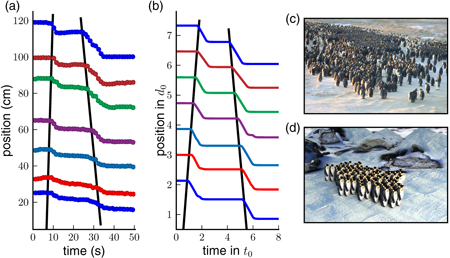
Figure 2. Comparison between the experiment and the simulation. (a) Penguin trajectories analyzed from the high-resolution images (Zitterbart et al [7]). The wave fronts (black lines) are running in different directions (positive or negative slope). (b) Trajectories of penguins in the simulation. (c) The snapshot of the video used for the extraction of the trajectories in (a) (see also movies 1 and 6 available from stacks.iop.org/NJP/15/125022/mmedia) taken from Zitterbart et al [7]). (d) Visualization of a huddle in the simulation (see also movie 5 available from stacks.iop.org/NJP/15/125022/mmedia).
Download figure:
Standard image High-resolution imageWe next explore the behavior in the huddle when a traveling wave was triggered simultaneously or in close succession at two distant sites. As the frequency 1/T = NRtr of the waves increases linearly with huddle size N, the resulting global velocity of the huddle could be naively expected to also grow linearly with the huddle size if each triggering event would cause the huddle to advance by one step. For larger huddles, the intermittent behavior would eventually vanish and the penguins would be in constant motion, a feature not observed in the video recordings [7] or in our simulations. Instead, we observe in our model that the fronts of two simultaneous waves do not pass through each other but merge. After the merged wave has traveled through the entire huddle, each individual penguin has performed only a single step, despite multiple overlapping triggering events. This interesting emergent effect is possible because wave propagation in a huddle is a nonlinear phenomenon so that the superposition principle (mutual cancelation or amplification of two waves) does not hold.
3.3. Wave speed
The wave speed through the huddle can be derived analytically (see appendix A) as the distance between two penguins, divided by the time t(dth) a penguin needs to move the threshold distance (figure 3). Hence, the wave speed depends only on the relative threshold distance dth/d0 and the maximum velocity vstep of a single penguin. Because the penguins face their nearest front neighbors at a 30° angle, the distance traveled during the time t(dth) is d0 cos(30°), and the ratio of the wave speed to the maximum velocity is

W0 is the Lambert W-function to take the acceleration of the forward step into account (see appendix A). Note that the acceleration and the threshold distance are not independent but are coupled, as explained above. The maximum velocity vstep, the wave speed vwave and the distance between the penguins d0 can be experimentally obtained (figure 2(a)), and from these values the threshold distance can be calculated according to equation (4). From the video recordings published in [7], we estimate a wave speed of around 12 cm s−1, a maximum velocity during the steps of 1–2 cm s−1 and a distance d0 of 34 cm. From these numbers we estimate a threshold distance dth of around 2 cm. Independently, a rough estimate of dth can also be directly obtained from the penguin trajectories as the amplitude of the distance fluctuations between two neighboring penguins during a step (see appendix B). From this, we find a value of dth = 1.84 ± 0.99 cm, which is similar to the value calculated from equation (4). Interestingly, this distance is comparable to twice the thickness of the compressive feather layer of around 1.2 cm [5]. This suggests that the penguins touch each other only slightly when standing in a huddle, without compressing the feather layer so as to maximize the huddle density without compromising their own insulation. More importantly, the analytical and the numerical results for the wave speed as a function of the threshold distance are nearly identical (figure 3).
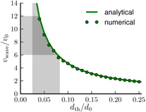
Figure 3. Comparison of the propagation speed of the traveling wave from the analytical solution (green line) and the numerical simulation (green circles). The wave speed depends on the threshold distance for triggering the wave. For the smaller thresholds, the wave travels faster. The gray shaded areas correspond to the range of the measured values from the video recordings for the relative wave speed and the relative threshold distance.
Download figure:
Standard image High-resolution image4. Features of the model
The traveling waves have been reported to have three main effects: global motion of the huddle, increasing the density of the huddle and allowing separate huddles to merge [7]. In the following, we explore whether our model also shows these features.
4.1. Maximizing density
High density requires a high degree of order in the huddle, ideally a strictly triangular lattice structure. Here, we test numerically how the huddle structure recovers from a disordered configuration. We distort a perfect triangular lattice with a lattice constant of d0 by randomly moving the individual penguins by a Gaussian distributed distance Δd in the x-direction, which is the direction the penguins are facing. We find that the disorder in the huddle, expressed as the standard deviation σ = stdev(dij), disappears quickly within t < 2t0, where t0 is the typical duration of a single step. This healing or annealing process takes place without the initiation of a traveling wave, and is driven only by the lattice disorder that causes the penguins to move according to equation (3). The residual degree of the disorder remains below the threshold distance (figure 4). Imperfections of σ > 0.25, however, do not heal spontaneously in our simulation for two reasons. Firstly, the rearrangements are so large that before some of the penguins have had a chance to find their ideal resting position, they have collided with another penguin and thus have triggered another wave of rearrangements. Secondly, the ideal positions, determined from the distance to the surrounding penguins, move at the same time and with a similar speed as the movement of each individual penguin. Thus, the huddle never comes to a rest. In real penguin huddles, we occasionally observe a complete break-up of the ordered huddle structure. However, it is at present not clear if this phenomenon is triggered by the large and ongoing movements of one or several penguins in the huddle.

Figure 4. (a) Time evolution of the disorder, expressed as the standard deviation of the distances (solid lines) for different starting conditions. The starting point is always a perfectly ordered huddle, but with different random shifts in the x-direction. From red to blue, the magnitude of the random shifts is increased. (b) Visualization of the starting conditions with different degrees of order (standard deviations of 0.01, 0.08, 0.16 and 0.25) (see movie 3, available from stacks.iop.org/NJP/15/125022/mmedia).
Download figure:
Standard image High-resolution image4.2. Merging of the huddles
In order to investigate how the model behaves when huddles merge, we start with two separate huddles some distance apart, both facing the same direction. If the waves are only initiated in the rear huddle, it approaches the huddle in front with every passing wave. Eventually, the rear huddle has covered the distance to the huddle in front, and as the two huddles touch, they merge seamlessly. All of the subsequent waves now pass through the united huddle (figure 5).

Figure 5. Kymograph showing the merging of the two huddles. Initially (top row), the two huddles are separated by a horizontal gap. Over time (top to bottom), the left huddle approaches the front huddle by a sequence of steps. Eventually (bottom row), the two huddles merge, and the waves travel through the merged huddle (see movie 4, available from stacks.iop.org/NJP/15/125022/mmedia).
Download figure:
Standard image High-resolution image4.3. Initiation of the waves
In the simulations, the penguins move only forward in the x-direction. This is similar to the situation in a traffic jam. Indeed, the reorganization waves in the penguin huddles closely resemble the stop-and-go waves and the intermittent behavior in jammed traffic. There are some fundamental differences, however: while in traffic jams the waves always start at the front of the queue and travel upstream from there, the waves in a penguin huddle can travel in both directions and also spread sideways in a rectangular pattern. Moreover, the waves in a penguin huddle can be triggered from any penguin regardless of its position. In particular, there is no need for a leading 'pacemaker' penguin in our model.
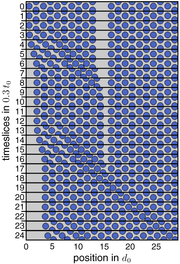
To test whether these results recapitulate the experimental findings, we perform an optical flow analysis of the video recordings of the penguin huddles. For this, we select a circular-shaped huddle in which the penguins face and move in the counter-clockwise direction around a stationary center (figure 6(a)). In this case, the lattice structure exhibits dislocation boundaries with a spiral pattern around the center, however over a shorter range, an approximately triangular order prevails. The optical flow is averaged in the y-direction (column-wise) over the lower half of the huddle to collapse the flow information onto a line (in the x-direction). The flow in the x-direction is then plotted versus time in a kymograph representation (figure 6(c)). Waves traveling from the left to the right side of the lower half of the huddle (in the direction of the penguin movements) are visible in the kymograph as lines with a negative slope. In the analogy, waves traveling from the right to the left against the direction of the penguin movements are visible in the kymograph as lines with a positive slope.

Figure 6. Optical flow analysis of the traveling wave dynamics. (a) Circular huddle with counter-clockwise (white arrow) rotational movements (copyright M Beaulieu and A Ancel, CNRS/IPEV). (b) Frame of the optical flow velocities in the huddle in (a). The flow velocity magnitude is column-wise averaged in the y-direction (orange arrow) over the lower half of the huddle (white dashed rectangle). The resulting line profile of the flow velocities along the x-direction (indicated by the red line) is plotted in the kymographs below. (c) The kymograph of the huddle movements during a 7 min period. White lines indicate wave fronts. Enlarged areas show (1) a decaying wave, (2) a non-decaying wave and (3) a merging event of two waves triggered at different positions. (d) Kymograph of the huddle movements in the simulation.
Download figure:
Standard image High-resolution imageThe occurrence of the positive and the negative slopes shows that the waves can travel forward and backwards through the huddle (figure 6(c)). Note that due to the larger lattice disorder in the case of a round huddle, the traveling waves may not always spread through the entire huddle but can die out over shorter distances (figure 6(c)1). The optical flow analysis also reveals that the waves start at different points in the huddle (corresponding to different y-positions in the kymograph). This leads to the conclusion that indeed the traveling waves can be triggered from different positions and therefore by different penguins in the huddle, which confirms the prediction of the model.
5. Conclusion
We present a simple model for the dynamical reorganization of emperor penguin huddles, based on an extension of the established one-dimensional models for traffic systems. Our model exhibits similarities with jammed traffic systems such as the stop-and-go waves and intermittent behavior, but also differences, such as that the waves can travel in all directions through a penguin huddle, which is confirmed here from the video recordings of the huddling penguins.
The model considers only the interactions between neighboring penguins, whereby a penguin moves to achieve or restore an optimal distance to the neighbors if this distance exceeds or falls below a threshold. Because each penguin is caged by surrounding penguins, a movement necessarily causes a propagation of the disturbances from the distance optimum and therefore leads to a traveling wave. The speed of the traveling wave depends on the optimal distance and the walking speed of the individual penguin, which both can be measured, and on the threshold distance, which can be inferred from the model. From our data, we estimate a threshold distance of 2 cm. We independently confirm this value from the fluctuations in the distances between the neighboring penguins during a traveling wave. Furthermore, the model confirms that the traveling waves help to achieve an optimally dense huddle structure, and describes how huddles can merge. More importantly, the model predicts that a traveling wave can be triggered from any penguin, regardless of its position in the huddle. This prediction is confirmed by an optical flow analysis of the video recordings from the huddling emperor penguins.
Acknowledgments
Field work at Durmont d'Urville during the winter of 2005 was financially and logistically supported by the Institut Polaire Français Paul-Emile Victor and the Terres Australes et Antarctiques Françaises. We also thank Yvon Le Maho, Céline Le Bohec, Achim Schilling and Adalbert Fono for encouragement, support and valuable discussions. This work was supported by DFG grant FA336/5-1.
Appendix A.: Analytical expression for the wave speed
The wave speed arises as a combination of the finite physical speed of the penguins during a forward step, and the instantaneous jump of the wave to the adjacent penguins after a threshold distance has been exceeded. This is in analogy to the saltatory propagation of the action potentials along the myelinated axons from one node of the Ranvier to the next node. In figure A.1 on the left side, a configuration of an undisturbed hexagonal packing is depicted, with a wave arriving from the left that has reached the rear penguins (cyan). These penguins now start moving to the right by a distance b, at which point they have pushed the desired position of the center penguin (red) beyond a critical distance dth. This situation is depicted in figure A.1 right. At this instance, the wave front jumps to the center penguin, which in turn starts moving to the right, and so forth. The effective wave speed is thus the time t(b) needed for the rear penguins (cyan) to move to the distance b, divided by the total distance  that the wave front has traveled during that time. Note that the rear penguins (cyan) continue to move beyond position b, but this has no further effect on the wave front.

Figure A.1. Schematic representation of the configurations of the penguins during wave propagation. (a) Starting configuration and (b) configuration after time t(b) at which the desired position (black cross) of the center penguin (red circle) has been moved by a threshold distance dth. As a consequence, the wave front jumps by a distance  .
.
Download figure:
Standard image High-resolution imageTo calculate the distance b, we first compute the positional error E(xi) as the sum of the squared neighbor distance errors
The desired position is the position of the minimum of E(xi)

We consider the origin of the coordinate system to be at the position of the central penguin. For the situation depicted in figure A.1(b) where the desired position of the central penguin has reached the threshold distance dth, the sum of the errors for the central penguin can be calculated from the positions of its six neighbors according to
Because in figure A.1(b) the penguin positions are symmetrical in y, we now can minimize this sum with respect to b to find the traveling distance b where the rear penguins have triggered the central penguin. The calculation is straightforward, and we find that btrigger = dth.
To calculate the time the rear penguins need to walk this distance of b, the differential equation for v

is integrated for the situation of a penguin starting at rest and accelerating to vdes = vstep.


Solving this equation for t gives

where W is the Lambert W-function.
The function t(x) gives the time for an accelerating penguin to walk the distance x. As shown above, to trigger the next step, the rear penguins have to walk the distance b = dth. For τ = dth/vstep, the time it takes the penguin to walk this distance is given by

When the rear penguins have triggered a step of the next penguin standing at a distance of  in front of it, the wave has traveled exactly this distance. The speed of the wave is


Appendix B.: Estimation of the threshold distance
To estimate the threshold distance, the video recordings of a densely packed region of the huddle [7] were analyzed. A section where a wave traveled backwards through the huddle was investigated. Neighboring pairs of penguins, one standing directly behind the other and both facing to the right, where chosen so that the x-component of the trajectory corresponds to the total distance traveled. For tracking, the upper corner of the white head spot was followed manually. The trajectories where then described with the equation

The parameters a, b, ts and te were fitted to the trajectories; m was chosen as  to describe a linear transition from the starting point of the step to the endpoint (figure B.1(b)).
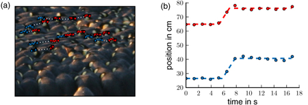
Figure B.1. (a) Snapshot of a video frame. The markers indicate the positions of the neighboring penguin pairs (connected by white dotted lines). The front penguin of a pair is labeled in red and the rear penguin in blue. (b) The fitted trajectory (dashed lines, fit according to equation (B.1)) of a pair of penguins. The circles represent the measured positions. From the fluctuations in the fitted distances between the neighboring penguins during a wave, the threshold distance dth can be estimated.
Download figure:
Standard image High-resolution imageThe distance between the neighboring penguins usually increases during a step because of the time shift in the initiation of the movement. This time shift arises from the reaction time and the finite speed that the front penguin travels to cover the threshold distance dth.
From the fitted pairs of the trajectories xi(t) and xj(t), the maximum distance max(xj–xi) between two neighboring penguins, normalized by the starting distance, was calculated. For an infinitely short reaction time, the threshold distance dth can then be calculated as

As the video material has a poor time resolution of 0.8 fps and the position of the tracked spot also can be determined only with the pixel resolution, the obtained value for dth = 0.054 ± 0.029 (mean ± std) pixels, corresponding to 1.84 ± 0.99 cm, should be regarded only as a rough estimate for this parameter.
Appendix C.: Assigning neighbors
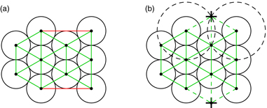
As discussed above in section 3.1, the choice of neighbors is important for calculating the desired position xdes. In the model, each penguin is assigned six direct neighbors as determined by the Delaunay triangulation [25]. However, care has to be taken with the penguins at the border of the huddle. Here, a simple Delaunay triangulation would link the penguins that are in no 'direct' neighborhood with each other (figure C.1(a)). Instead, we perform a Delaunay triangulation after including additional points (virtual penguins) outside the border of the huddle. To construct these points, a circle with radius 2ri is drawn around every border penguins i, and the points where two such circles intersect are selected. If a point falls within the desired region of an existing penguin, i.e. it is less than rj away from a penguin j, it is rejected (figure C.1(b)). As the huddles can merge and thus the boundary of a huddle can change, these additional points are recalculated for every frame.
Figure C.1. (a) Neighbor assignments obtained by simple Delaunay triangulation. In addition to the desired assignments (green), some far away penguins are also connected (red). (b) Drawing a circle around every penguin and inserting points (crosses) at the intersections eliminates the undesired connections.
Download figure:
Standard image High-resolution image