


Abstract
A system with unequal populations of up and down fermions may exhibit a Larkin–Ovchinnikov (LO) phase characterized by periodic domain walls across which the order parameter changes sign and the excess polarization is localized. Despite fifty years of theoretical and experimental work, there has so far been no unambiguous observation of an LO phase. Here we propose an experiment in which two fermion clouds, prepared with unequal population imbalances, are allowed to expand and interfere. We show that a pattern of staggered fringes in the interference is unequivocal evidence of LO physics.
Export citation and abstract BibTeX RIS
1. Introduction
As a fascinating example of self-organized quantum matter, Fulde–Ferrell–Larkin–Ovchinnikov (FFLO) states have long been sought after in exotic superconductors [1, 2] and in ultracold atomic gases [3], and they may even occur in neutron stars [4]. In superconductors, modulated superfluidity results from the interplay between superconducting pairs and an applied parallel magnetic field. The inter-electron attraction favors a superfluid (SF) state consisting of pairs of up- and down-spin electrons, whereas the field favors a polarized Fermi liquid (FL) state with a lower Zeeman energy. The simplest theories predict a first-order SF–FL transition [5, 6]. However, the competition between pairing and polarization can produce far more subtle physics—an intermediate FFLO state [7–12], henceforth referred to as LO4, as depicted in figure 1. As the field is increased beyond hc1 it forces excess fermions into the SF in the form of domain walls where the order parameter changes sign between positive and negative values. (This is analogous to how a perpendicular field forces vortices into a superconducting film.) The wavelength of these modulations decreases with increasing field and ultimately the system gives way to a polarized Fermi liquid.

Figure 1. Top: schematic of a fully paired SF, an LO state with excess fermions in domain walls, and a polarized Fermi liquid. Center: pairing amplitude Δ and magnetization m as a function of the Zeeman field h, which is the difference between the chemical potentials of up and down spins. The LO phase exists in a field range hc1 < h < hc2. Bottom: real space behavior of Δ(x) and m(x) in each phase.
Download figure:
Standard imageCold atom experiments provide a highly tunable testing ground for finding LO states, and there have been several proposals to do so through modulations of the polarization in real space [12], peaks in the pair momentum distribution at the modulation wavevector [13, 14], shadow features in the single-particle momentum distribution [12], and Andreev bound states in the density of states [12]. A recent experiment on an array of one-dimensional (1D) tubes found density profiles in agreement with Bethe ansatz calculations [15], which predict power-law LO correlations at zero temperature. However, direct evidence of the sign changes of the order parameter—the defining feature of an LO state—is still lacking.
In this paper, we propose an interference experiment in which two isolated SFs expand into each other, as illustrated in figure 2. The ideal situation for detecting the LO phase is shown in the lower panel of this figure, where one layer is a uniform fully-paired SF, which serves as a reference phase, and the other layer is a modulated (LO) SF. The resulting interference pattern is directly sensitive to real-space modulations of the order parameter, and should provide an unequivocal signature of the elusive LO phase.
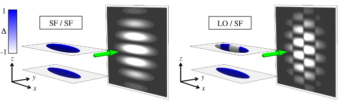
Figure 2. Principle of our cold atom interference experiment. Two cigar-shaped condensates are allowed to expand. After a suitable time-of-flight, the shadow of a probe laser in the y-direction gives the interference pattern projected onto the x–z plane. If both clouds are in the uniform SF phase, the interference pattern is similar to the familiar double-slit experiment (left). In contrast, interference between an LO phase and a SF phase gives staggered fringes (right).
Download figure:
Standard image2. Experimental proposal
LO states have been predicted to exist in various situations [12, 16, 17]. The most likely of these to be realized in the near future is an array of tubes with a small intertube coupling [13, 18, 19]. This quasi-1D geometry provides good Fermi surface nesting at the LO wavevector qLO = kF↑ − kF↓, together with Josephson coupling between the order parameter in adjacent tubes which is necessary to stabilize true long-range order.
Therefore, it seems that the idea can be best realized in the following way. Two species of fermions (referred to as ↑ and ↓) are loaded into an optical trap. The cloud is separated into two independent quasi-2D 'pancake' layers using an optical lattice with a wide spacing in the vertical direction z (created with two laser beams intersecting at a shallow angle [20]). In order to generate an LO phase it is necessary for the two layers to have different relative population imbalances. This may happen by chance due to natural number fluctuations, or alternatively, one can induce hyperfine transitions using Raman transitions, where the two lasers are detuned at the appropriate RF frequency. In order to address each layer separately, it would be necessary to make the beam diameters smaller than the interlayer distance. In this paper, we do the analysis of the interference patterns assuming that one of the layers is balanced while the other contains a population imbalance, but this is not necessary. As long as there are different relative population imbalances between the two layers, LO signatures will be observable. An additional optical lattice is further used to create a 2D array of weakly-coupled tubes, conducive to the formation of an LO state. The resulting geometry is shown in figure 3.
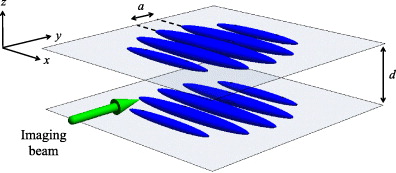
Figure 3. Proposed experimental geometry. The fermion gas is confined in a harmonic trap. An optical lattice with a large spacing in the z-direction is used to separate the gas into two independent quasi-2D layers. A second optical lattice in the y-direction cuts each layer into a series of weakly coupled tubes—the optimal geometry for LO physics. The trap and lattices are turned off abruptly, allowing the two layers to expand and interfere with one another, generating fringes as in figure 2.
Download figure:
Standard imageOnce the gases are allowed to equilibrate for sufficient time, the interactions in the system are quickly ramped to the Bose–Einstein condensate (BEC) side of the Feshbach resonance [21] to 'freeze' or 'project' the pair wavefunction into a boson wavefunction, so that from this point onwards the pairs move as independent bosons (instead of disintegrating into fermions). Then, the confining potentials are abruptly turned off. As the clouds expand into one another, they interfere and form a 3D matter wave interference pattern. The projection of this interference pattern onto the x-z plane can be measured by absorption of a resonant probe beam along the y direction. Any LO phase modulation features will be captured in these projected interference patterns. It may be desirable to image the minority (↓) atoms, which gives the final distribution of the tightly bound pairs without contamination from unpaired majority (↑) atoms.
An earlier paper [22] has discussed the interferometric detection of the FFLO phase through correlation functions [23, 24] obtained by averaging over many interference snapshots. We emphasize that our proposal considers the information in the individual snapshots themselves, most notably the 'tire-tread' staggered interference fringes corresponding to the sign change of the paring amplitude across the domain walls. The information in these individual snapshots contains distinct information from that in the correlation functions. For example, if the domain wall spacing is not uniform in multiple snapshots, possibly due to density fluctuations between different tubes, the LO information could be lost in the averaging necessary to obtain correlation function data.
3. Interference between coupled tubes
We now discuss analytically the salient features of the interference patterns of a 2D array of coupled tubes. We begin by considering two layers, each containing N coupled tubes, with separation d in the z-direction. After ramping up the interaction to produce a molecular BEC (of fermion pairs), the wavefunction is
where a is the separation between in-plane tubes and σy and σz are the Gaussian confinements in the respective directions. The wavefunction in the nth tube is denoted by ΔTn(x) in the top layer and by ΔBn(x) in the bottom layer. When the trap and lattices are switched off, the clouds expand predominantly in the tightly confined directions (y and z). After a suitable time-of-flight t, the wavefunction is effectively Fourier-transformed in the y and z directions. That is, the final wavefunction Δ(x,y,z,t) is approximately proportional to the initial momentum distribution in the y and z directions, i.e. Δ(x,y,z,t) ≈ Δ(x,ky,kz,t = 0) where y = tky/m and z = tkz/m:
The 3D density of the cloud, after expansion, is given by I(x,ky,kz)∝|Δ(x,ky,kz)|2. The imaging process measures the integrated density along the y direction,  :
:
We can consider the behavior of the above interference formula in its two limits: widely separated tubes (a/σy → ∞) and overlapping tubes (a/σy → 0). In the overlapping limit, the total interference pattern reduces to that of two isolated 2D layers. In the limit of widely separated tubes, similar to the proposed experiment, the total interference pattern reduces to the sum of the interference patterns from adjacent tubes in the two layers.
Realistic parameters are interlayer spacing d = 3 μm, layer thickness σz ≈ 200 nm, and optical lattice spacing 532 nm in the y direction [15, 20]. This lattice should be shallow enough to allow sufficient intertube hopping to lock the position of domain walls between adjacent tubes. Our analysis is valid when the domain wall spacing is much larger than σz, which is true for small imbalances.
The above analysis involves just two layers, which are necessary and sufficient for generating interference. Introducing more layers would complicate the analysis, and reduce the visibility of the interference pattern5; nevertheless, there would still be observable effects of the order of  .
.
Figure 4 illustrates the projected interference pattern, described by equation (3), for three configurations of the upper layer: a uniform SF, an LO phase with domain walls locked between tubes, and an LO phase with domain walls fluctuating between tubes. In each case we assume that the lower layer has been prepared in a uniform SF state. The form of the LO state that we use is the Jacobi elliptic function sn(x|k), which is a good approximation of the pair wavefunction in the limit of quasi-1D tubes with small intertube coupling [25]. Each wavefunction is multiplied by Gaussian envelopes in the x, y, and z directions to mimic the effect of the trapping potential. The staggered fringe pattern in the lower two panels is a clear signature of oscillations of the relative phase between the SF and LO layers, in contrast to the straight interference fringes in the top panel.

Figure 4. Interference patterns for three different configurations: fully paired SF state (top left), locked LO state (top right), and unlocked LO state (bottom). In each case we consider a 2 × 5 array of coupled tubes as shown in figure 3, using a fully paired SF as a reference phase in the bottom layer. The pairing amplitude Δ(x) in each of the five top layer tubes is shown to the left of the interference pattern. The locked LO states were taken to be Δ(x) = e−x2/2σ2
sn(x/λLO|k), for  with period λLO, where sn(x|k) is the Jacobi elliptic function. In the unlocked case we added a random displacement of the domain walls Δ(x) = e−x2/2σ2
sn((x + δ)/λLO|k) where δ∈[ − λLO,λLO]. This interference pattern contains signatures of the LO phase even when the domain wall locations fluctuate between tubes. In the bottom right, we show fixed-z cuts of the interference pattern for the fully locked LO state (top) and unlocked LO state (bottom). For the locked domain walls, the original domain wall spacing λLO is the same as the peak-to-peak distance of the horizontal interference fringes (since there is no expansion in the x-direction). While the visibility is reduced in the unlocked case, from the peak-to-peak distance we can still identify the domain wall spacing.
with period λLO, where sn(x|k) is the Jacobi elliptic function. In the unlocked case we added a random displacement of the domain walls Δ(x) = e−x2/2σ2
sn((x + δ)/λLO|k) where δ∈[ − λLO,λLO]. This interference pattern contains signatures of the LO phase even when the domain wall locations fluctuate between tubes. In the bottom right, we show fixed-z cuts of the interference pattern for the fully locked LO state (top) and unlocked LO state (bottom). For the locked domain walls, the original domain wall spacing λLO is the same as the peak-to-peak distance of the horizontal interference fringes (since there is no expansion in the x-direction). While the visibility is reduced in the unlocked case, from the peak-to-peak distance we can still identify the domain wall spacing.
Download figure:
Standard image4. Time-of-flight simulation
To better understand how the interference pattern evolves once the trapping potentials have been switched off, we have simulated the time-of-flight evolution of our experimental setup. To do this, we numerically evolve the free-particle Schrödinger equation

subject to the initial pairing amplitude when the trap is abruptly turned off (t = 0).
We have analyzed the evolution of the interference pattern for a two-tube geometry similar to what is shown in the right panel of figure 2, where one of the tubes is in a fully paired SF state and the adjacent tube is in an LO state. The LO state we used is the same as that used in the analysis of figure 4 above. This provides the opportunity to test the validity of the approximation that we need to only consider expansion in the two transverse directions, and that a suitable time-of-flight can be found in experiments that achieves this 'far field' limit. The results of our simulation are shown in figure 5. To set the time and length scales, we have set the length of our tubes to be approximately 50 μm, and used the mass of 6Li, typical values for such an experiment [15]. The spacing of the domain walls is about 10 μm, which is also the spacing of the bright and dark interference signals in the horizontal direction. This length scale is accessible in similar time-of-flight experiments [26] that have a resolution of ≈3 μm. In the central panel of figure 5, we see that there is a suitable intermediate time-of-flight where expansion in the longitudinal (x) direction can be neglected, and the interference patterns shown in figure 4 are valid. The expansion time of this snapshot is t ≈ mdR⊥/ℏ, where d is the separation of the tubes and R⊥ is the transverse radius of the tube, can be associated with the 'far field' limit of expansion in the transverse (z) direction [27].

Figure 5. Interference patterns I∝|Δ(x,z)|2 obtained from time-of-flight simulations. The initial configuration (left) consists of a fully paired SF in the upper tube and an LO state in the lower tube. The domain walls characterizing the LO state can be seen in the figure. After a suitable intermediate time-of-flight expansion, the interference pattern develops with no significant expansion in the longitudinal (x) direction (center) consistent with the analysis above, and staggered interference fringes are clearly visible. For longer times, expansion along the x-axis occurs, but LO signatures remain (right).
Download figure:
Standard imageOur simulations also allow us to comment on the effects of expansion along the x-axis in our experimental proposal. In the final frame of figure 5, we show the interference pattern after long time expansion. Despite the fact that the analysis of section 3 for the interference pattern breaks down in this regime, the LO interference signatures remain visible.
Our time-of-flight simulation contains two isolated tubes for computational simplicity. In the experiment proposed above, we have considered an array of coupled tubes in order to quench the fluctuations. The time-of-flight calculation can be extended to an array of tubes, similar to the proposed experiment. In this geometry, the expansion in the y-direction would approach the far-field limit at times ty ≈ maR⊥/ℏ. Since a ≈ d/6, ty < tz = mdR⊥/ℏ which implies that when the far-field limit is satisfied in the z-direction, the far-field limit is also satisfied in the y-direction, and the analysis discussed in section 3 is valid.
5. Discussion
Even with intertube coupling to stabilize quasi-long-range-order, we expect thermal and quantum fluctuations to have an impact on the interference patterns in our proposed experiment.
5.1. Thermal fluctuations
The interference experiment that we have proposed essentially takes 'snapshots' of the wavefunction after the time-of-flight. For this reason, the thermal phase fluctuations are not integrated over, and can be considered as domain wall fluctuations between tubes. However, as shown in the lowest panel of figure 4, these fluctuations are not severe enough to destroy the occurrence of staggered interference fringes, the signature of an LO phase. This is further detailed in the bottom right panel of the same figure, where we show a cross section of the interference pattern.
A remarkable feature of cold atom experiments is that control parameters (interaction, lattice depth, and trap depth) can be turned off very quickly, much faster than the typical timescale of domain wall movement. This allows us to take a snapshot of the wavefunction (resolved in real time), in a way not possible in condensed matter experiments. Thus, even above the critical temperature where thermal fluctuations destroy long-range order, it may still be possible to detect LO physics in the form of 'temporary' domain walls!
In order to study the effect of thermal fluctuations quantitatively, we have performed Bogoliubov–de Gennes (BdG) simulations of the 2D attractive Hubbard Hamiltonian


with hopping trr' = t for nearest-neighbor bonds along the length of the tube (in the x direction), trr' = t⊥ for nearest-neighbor bonds between tubes, fermion creation and annihilation operators c†rσ and crσ, number operators nrσ = c†rσcrσ, chemical potentials μσ = μ − σh for the two spin species, Zeeman field h, local Hubbard attraction  , and confining harmonic potential Vr.
The results of these simulations on a system of 7 tubes with 50 sites in each tube are shown in figure 6. The harmonic potential we consider mimics the experimental proposal. The behavior of the BdG pairing amplitude  in the central three tubes as a function of temperature for intertube coupling strengths t⊥ = 0.1t and 0.3t is shown. For small intertube coupling t⊥/t = 0.1, we see domain wall fluctuations between the tubes whose effect we have included in our interference pattern analysis in figure 4. As the intertube coupling is increased at low temperatures, the phases of the domain walls in the different tubes 'lock' together. Our BdG results show that the LO state survives up to a temperature of TLO ≈ 0.12t. We expect phase fluctuations to suppress TLO and to also depend on the intertube coupling; the larger the coupling, the smaller the suppression. However, as we have emphasized above, in spite of these fluctuations, the interferometric signature would still be visible up to T* ∼ TLO (which is a significant fraction of the temperature for the onset of pairing TBCS ≈ 0.2t for these parameters).
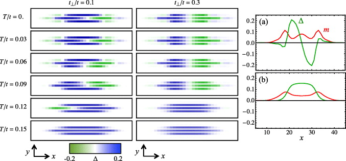
Figure 6. Results of BdG simulations on a 50 × 7 lattice in a harmonic potential Vr. The parameters for the system are  and μavg = 0.1t, with harmonic potential
  , where the origin is at the center of the lattice. Left: pairing amplitude Δ for intertube coupling strengths t⊥/t = 0.1 and 0.3. At low temperatures, an LO state is seen in the central three tubes of the trap for T < 0.12t. Thermal domain wall fluctuations similar to those studied in figure 4 can be seen in the simulations with small intertube coupling t⊥/t = 0.1. With increasing intertube coupling, the LO domain wall phases become locked between the different tubes. Right: pairing amplitude Δ and magnetization m in the central tube for t⊥/t = 0.3 at T = 0 (a) and T = 0.15t (b). Because of the harmonic confinement, the excess magnetization can reside in the wings of the trap for both the LO and BCS states, but for the LO state (a), there are also peaks in m at the LO domain walls.
Download figure:
Standard image5.2. Quantum fluctuations
At low temperatures, the excess fermions residing in the domain walls quantum tunnel from one position to another. This can be viewed as the diffusion of domain walls in imaginary time τ; measurements are necessarily averaged over τ. For isolated tubes, quantum fluctuations of the domain walls prevent long-range LO order, and there is only quasi-long-range order at zero temperature; hence, the interference pattern will be washed out. This is why we recommend using sufficient coupling between the tubes to lock their phases so that the pairing amplitude modulations remain even after averaging over quantum fluctuations (see figure 7).
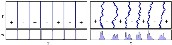
Figure 7. lllustration of imaginary time worldlines of LO domain walls and corresponding magnetizations with (right) and without (left) quantum fluctuations. Pluses and minuses correspond to the sign of the pairing amplitude Δ(x) in each region. In the bottom panel, the quantum fluctuations enforce a spatial profile for the magnetization that is less sharp, but which still clearly maintains the features of domain walls.
Download figure:
Standard image5.3. Stabilization of fluctuations with intertube coupling
It is known that in 1D systems at finite temperatures, there is no long-range-order. Indeed, interference experiments between two quasi-1D systems have demonstrated the exponential decay of correlations in the system [26, 28]. Here again, we emphasize that our proposal suggests that experimentalists look at the interference between planes of coupled 1D tubes, which has the effect of stabilizing the LO order. Although this order at finite temperatures is only algebraic at best (since the planes are still 2D), the system is effectively long range ordered if the correlation length is larger than the system size. Similar experiments on 2D Bose systems [20] have found 'zipper' interference patterns which were attributed to unbound vortex-antivortex pairs. These vortex/antivortex fluctuations are only observed near the Kosterlitz–Thouless transition. In contrast, domain walls are an integral feature of the LO ground state and should exist in the whole temperature range 0 < T < Tc.
In our experimental geometry it is easy to distinguish between the interference signatures of the vortices and LO domain wall defects. Since vortices are point defects in 2D, they will produce interference signatures regardless of the direction of the imaging beam. In particular, if the imaging beam were positioned along the axis of the tubes (the x direction), LO signatures would disappear and vortex signatures, if they were to occur, would be visible. Regardless, we do not expect vortices like those seen in the 2D Bose gas experiments to occur because the coupling between tubes is small.
5.4. Conclusions
Interferometric techniques have proven to be powerful methods to detect the internal structure of the pairs in cuprates [29], ruthenates, pnictides, and other unconventional superconductors [30]. Our proposal differs from those experiments in that it measures the sign changes of the order parameter as a function of the center of mass of the pairs. Such a measurement would be the first to directly image the real space modulation predicted for the LO phase and provide unequivocal evidence of LO physics.
Acknowledgments
We gratefully acknowledge useful discussions with Randy Hulet. This work was supported by ARO grant numbers W911NF-08-1-0338 (NT) and DARPA grant no. 60025344 under the Optical Lattice Emulator (OLE) program (YLL and NT). MS acknowledges support from the NSF Graduate Research Fellowship Program.
Footnotes
- 4
- 5
In fact, a three-layer geometry has the advantage that the central layer and outer layers naturally acquire different population imbalances when loaded. We have checked that this geometry still produces visible fringes.