
Abstract
Interstellar is the first Hollywood movie to attempt depicting a black hole as it would actually be seen by somebody nearby. For this, our team at Double Negative Visual Effects, in collaboration with physicist Kip Thorne, developed a code called Double Negative Gravitational Renderer (DNGR) to solve the equations for ray-bundle (light-beam) propagation through the curved spacetime of a spinning (Kerr) black hole, and to render IMAX-quality, rapidly changing images. Our ray-bundle techniques were crucial for achieving IMAX-quality smoothness without flickering; and they differ from physicists' image-generation techniques (which generally rely on individual light rays rather than ray bundles), and also differ from techniques previously used in the film industry's CGI community. This paper has four purposes: (i) to describe DNGR for physicists and CGI practitioners, who may find interesting and useful some of our unconventional techniques. (ii) To present the equations we use, when the camera is in arbitrary motion at an arbitrary location near a Kerr black hole, for mapping light sources to camera images via elliptical ray bundles. (iii) To describe new insights, from DNGR, into gravitational lensing when the camera is near the spinning black hole, rather than far away as in almost all prior studies; we focus on the shapes, sizes and influence of caustics and critical curves, the creation and annihilation of stellar images, the pattern of multiple images, and the influence of almost-trapped light rays, and we find similar results to the more familiar case of a camera far from the hole. (iv) To describe how the images of the black hole Gargantua and its accretion disk, in the movie Interstellar, were generated with DNGR—including, especially, the influences of (a) colour changes due to doppler and gravitational frequency shifts, (b) intensity changes due to the frequency shifts, (c) simulated camera lens flare, and (d) decisions that the film makers made about these influences and about the Gargantua's spin, with the goal of producing images understandable for a mass audience. There are no new astrophysical insights in this accretion-disk section of the paper, but disk novices may find it pedagogically interesting, and movie buffs may find its discussions of Interstellar interesting.
Export citation and abstract BibTeX RIS

Content from this work may be used under the terms of the Creative Commons Attribution 3.0 licence. Any further distribution of this work must maintain attribution to the author(s) and the title of the work, journal citation and DOI.
1. Introduction and overview
1.1. Previous research and visualizations
At a summer school in Les Houches, France, in summer 1972, Bardeen [1], building on earlier work of Carter [2], initiated research on gravitational lensing by spinning black holes. Bardeen gave a thorough analytical analysis of null geodesics (light-ray propagation) around a spinning black hole; and, as part of his analysis, he computed how a black hole's spin affects the shape of the shadow that the hole casts on light from a distant star field. The shadow bulges out on the side of the hole moving away from the observer, and squeezes inward and flattens on the side moving toward the observer. The result, for a maximally spinning hole viewed from afar, is a D-shaped shadow; cf figure 4. (When viewed up close, the shadow's flat edge has a shallow notch cut out of it, as hinted by figure 8.)
Despite this early work, gravitational lensing by black holes remained a backwater of physics research until decades later, when the prospect for actual observations brought it to the fore.
There were, we think, two especially memorable accomplishments in the backwater era. The first was a 1978 simulation of what a camera sees as it orbits a non-spinning black hole, with a star field in the background. This simulation was carried out by Palmer et al [3] on an Evans and Sutherland vector graphics display at Simon Fraser University. Palmer et al did not publish their simulation, but they showed a film clip from it in a number of lectures in that era. The nicest modern-era film clip of this same sort that we know of is by Riazuelo (contained in his DVD [4] and available on the web at [5]); see figure 3 and associated discussion. And see [6] for an online application by Müller and Weiskopf for generating similar film clips. Also of much interest in our modern era are film clips by Hamilton [7] of what a camera sees when falling into a nonspinning black hole; these have been shown at many planetariums, and elsewhere.
The other most memorable backwater-era accomplishment was a black and white simulation by Luminet [8] of what a thin accretion disk, gravitationally lensed by a nonspinning black hole, would look like as seen from far away but close enough to resolve the image. In figure 15(c), we show a modern-era colour version of this, with the camera close to a fast-spinning black hole.
Gravitational lensing by black holes began to be observationally important in the 1990s. Rauch and Blandford [9] recognized that, when a hot spot, in a black hole's accretion disk or jet, passes through caustics of the Earth's past light cone (caustics produced by the hole's spacetime curvature), the brightness of the hot spot's x-rays will undergo sharp oscillations with informative shapes. This has motivated a number of quantitative studies of the Kerr metric's caustics; see, especially [9–11] and references therein.
These papers' caustics are relevant for a source near the black hole and an observer far away, on Earth—in effect, on the black hole's 'celestial sphere' at radius  . In our paper, by contrast, we are interested in light sources that are usually on the celestial sphere and an observer or camera near the black hole. For this reversed case, we shall discuss the relevant caustics in sections 3.3 and 3.4. This case has been little studied, as it is of primarily cultural interest ('everyone' wants to know what it would look like to live near a black hole, but nobody expects to make such observations in his or her lifetime), and of science-fiction interest. Our paper initiates the detailed study of this culturally interesting case; but we leave a full, systematic study to future research. Most importantly, we keep our camera outside the ergosphere—by contrast with Riazuelo's [12] and Hamilton's [7] recent simulations with cameras deep inside the ergosphere and even plunging through the horizon3
.
. In our paper, by contrast, we are interested in light sources that are usually on the celestial sphere and an observer or camera near the black hole. For this reversed case, we shall discuss the relevant caustics in sections 3.3 and 3.4. This case has been little studied, as it is of primarily cultural interest ('everyone' wants to know what it would look like to live near a black hole, but nobody expects to make such observations in his or her lifetime), and of science-fiction interest. Our paper initiates the detailed study of this culturally interesting case; but we leave a full, systematic study to future research. Most importantly, we keep our camera outside the ergosphere—by contrast with Riazuelo's [12] and Hamilton's [7] recent simulations with cameras deep inside the ergosphere and even plunging through the horizon3
.
In the 1990s astrophysicists began to envision an era in which very long baseline interferometry would make possible the imaging of black holes—specifically, their shadows and their accretion disks. This motivated visualizations, with ever increasing sophistication, of accretion disks around black holes: modern variants of Luminet's [8] pioneering work. See, especially, Fukue and Yokoyama [13], who added colours to the disk; Viergutz [14], who made his black hole spin, treated thick disks, and produced particularly nice and interesting coloured images and included the disk's secondary image which wraps under the black hole; Marck [15], who laid the foundations for a lovely movie now available on the web [16] with the camera moving around close to the disk, and who also included higher-order images, as did Fanton et al [17] and Beckwith and Done [18]. See also papers cited in these articles.
In the 2000s astrophysicists have focused on perfecting the mm-interferometer imaging of black-hole shadows and disks, particularly the black hole at the centre of our own Milky Way Galaxy (Sgr A*). See, e.g., the 2000 feasibility study by Falcke et al [19]. See also references on the development and exploitation of general relativistic magnetohydrodynamical (GRMHD) simulation codes for modelling accretion disks like that in Sgr A* [20–22]; and references on detailed GRMHD models of Sgr A* and the models' comparison with observations [23–26]. This is culminating in a mm interferometric system called the Event Horizon Telescope [27], which is beginning to yield interesting observational results though not yet full images of the shadow and disk in Sgr A*.
All the astrophysical visualizations of gravitational lensing and accretion disks described above, and all others that we are aware of, are based on tracing huge numbers of light rays through curved spacetime. A primary goal of today's state-of-the-art, astrophysical ray-tracing codes (e.g., the Chan et al massively parallel, GPU-based code GRay [28]) is very fast throughput, measured, e.g., in integration steps per second; the spatial smoothness of images has been only a secondary concern. For our Interstellar work, by contrast, a primary goal is smoothness of the images, so flickering is minimized when objects move rapidly across an IMAX screen; fast throughput has been only a secondary concern.
With these different primary goals, in our own code, called Double Negative Gravitational Renderer (DNGR), we have been driven to employ a different set of visualization techniques from those of the astrophysics community—techniques based on propagation of ray bundles (light beams) instead of discrete light rays, and on carefully designed spatial filtering to smooth the overlaps of neighbouring beams; see section 2 and appendix
In appendix
1.2. This paper
Our work on gravitational lensing by black holes began in May 2013, when Christopher Nolan asked us to collaborate on building realistic images of a spinning black hole and its disk, with IMAX resolution, for his science-fiction movie Interstellar. We saw this not only as an opportunity to bring realistic black holes into the Hollywood arena, but also an opportunity to create a simulation code capable of exploring a black hole's lensing with a level of image smoothness and dynamics not previously available.
To achieve IMAX quality (with 23 million pixels per image and adequately smooth transitions between pixels), our code needed to integrate not only rays (photon trajectories) from the light source to the simulated camera, but also bundles of rays (light beams) with filtering to smooth the beams' overlap; see section 2, appendices
Thorne, having had a bit of experience with this kind of stuff, put together a step-by-step prescription for how to map a light ray and ray bundle from the light source (the celestial sphere or an accretion disk) to the camera's local sky; see appendices
In section 3, we use this code to explore a few interesting aspects of the lensing of a star field as viewed by a camera that moves around a fast-spinning black hole (0.999 of maximal—a value beyond which natural spin-down processes become strong [31]). We compute the intersection of the celestial sphere  with the primary, secondary, and tertiary caustics of the camera's past light cone and explore how the sizes and shapes of the resulting caustic curves change as the camera moves closer to the hole and as we go from the primary caustic to higher-order caustics. We compute the images of the first three caustics on the camera's local sky (the first three critical curves), and we explore in detail the creation and annihilation of stellar-image pairs, on the secondary critical curve, when a star passes twice through the secondary caustic. We examine the tracks of stellar images on the camera's local sky as the camera orbits the black hole in its equatorial plane. And we discover and explain why, as seen by a camera orbiting a fast spinning black hole in our Galaxy, there is just one image of the galactic plane between adjacent critical curves near the poles of the black hole's shadow, but there are multiple images between critical curves near the flat, equatorial shadow edge. The key to this from one viewpoint is the fact that higher-order caustics wrap around the celestial sphere multiple times, and from another viewpoint the key is light rays temporarily trapped in prograde, almost circular orbits around the black hole. By placing a checkerboard of paint swatches on the celestial sphere, we explore in detail the overall gravitational lensing patterns seen by a camera near a fast-spinning black hole and the influence of aberration due to the camera's motion.
Whereas most of section 3 on lensing of stellar images is new, in the context of a camera near the hole and stars far away, our section 4, on lensing of an accretion disk, retreads largely known ground. But it does so in the context of the movie Interstellar, to help readers understand the movie's black-hole images, and does so in a manner that may be pedagogically interesting. We begin with a picture of a gravitationally lensed disk made of equally spaced paint swatches. This picture is useful for understanding the multiple images of the disk that wrap over and under and in front of the hole's shadow. We then replace the paint-swatch disk by a fairly realistic and rather thin disk (though one constructed by Double Negative artists instead of by solving astrophysicists' equations for thin accretion disks [32]). We first compute the lensing of our semi-realistic disk but ignore Doppler shifts and gravitational redshifts, which we then turn on pedagogically in two steps: the colour shifts and then the intensity shifts. We discuss why Christopher Nolan and Paul Franklin chose to omit the Doppler shifts in the movie, and chose to slow the black hole's spin from that,  , required to explain the huge time losses in Interstellar, to
  . And we then discuss and add simulated lens flare (light scattering and diffraction in the camera's lenses) for an IMAX camera that observes the disk—something an astrophysicist would not want to do because it hides the physics of the disk and the lensed galaxy beyond it, but that is standard in movies, so computer generated images will have continuity with images shot by real cameras.
Finally, in section 5 we summarize and we point to our use of DNGR to produce images of gravitational lensing by wormholes.
Throughout we use geometrized units in which G (Newton's gravitation constant) and c (the speed of light) are set to unity, and we use the MTW sign conventions [33].
2. DNGR: our Double Negative Gravitational Renderer code
Our computer code for making images of what a camera would see in the vicinity of a black hole or wormhole is called the Double Negative Gravitational Renderer, or DNGR—which obviously can also be interpreted as the Double Negative General Relativistic code.
2.1. Ray tracing
The ray tracing part of DNGR produces a map from the celestial sphere (or the surface of an accretion disk) to the camera's local sky. More specifically (see appendix
- (i)In DNGR, we adopt Boyer–Lindquist coordinates
 for the black hole's Kerr spacetime. At each event we introduce the locally non-rotating observer, also called the fiducial observer (FIDO) in the membrane paradigm [34]: the observer whose four-velocity is orthogonal to the surfaces of constant t, the Kerr metric's space slices. We regard the FIDO as at rest in space, and give the FIDO orthonormal basis vectors, , that point along the spatial coordinate lines.
 - (ii)We specify the camera's coordinate location; its direction of motion relative to the FIDO there, a unit vector in the camera's reference frame; and the camera's speed β relative to the FIDO.
- (iii)In the camera's reference frame, we set up a right-handed set of three orthonormal basis vectors, with along the direction of the camera's motion, perpendicular to and in the plane spanned by and , and orthogonal to and . See figure 1. And we then set up a spherical polar coordinate system for the camera's local sky (i.e. for the directions of incoming light rays) in the usual manner dictated by the camera's Cartesian basis vectors .
- (iv)For a ray that originates on the celestial sphere (at), we denote the Boyer–Lindquist angular location at which it originates by .
- (v)We integrate the null geodesic equation to propagate the ray from the camera to the celestial sphere, thereby obtaining the map of points on the camera's local sky to points on the celestial sphere.
- (vi)If the ray originates on the surface of an accretion disk, we integrate the null geodesic equation backward from the camera until it hits the disk's surface, and thereby deduce the map from a point on the disk's surface to one on the camera's sky. For more details on this case, see appendix
A.6 . - (vii)We also compute, using the relevant Doppler shift and gravitational redshift, the net frequency shift from the ray's source to the camera, and the corresponding net change in light intensity.


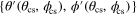

Figure 1. The mapping of the camera's local sky  onto the celestial sphere
  via a backward directed light ray; and the evolution of a ray bundle, that is circular at the camera, backward along the ray to its origin, an ellipse on the celestial sphere.
Download figure:
Standard image High-resolution image2.2. Ray-bundle (light-beam) propagation
DNGR achieves its IMAX-quality images by integrating a bundle of light rays (a light beam) backward along the null geodesic from the camera to the celestial sphere using a slightly modified variant of a procedure formulated in the 1970s by Pineault and Roeder [35, 36]. This procedure is based on the equation of geodesic deviation and is equivalent to the optical scalar equations [37] that have been widely used by astrophysicists in analytical (but not numerical) studies of gravitational lensing; see references in section 2.3 of [38]. Our procedure, in brief outline, is this (see figure 1); for full details, see appendix
- (i)In DNGR, we begin with an initially circular (or sometimes initially elliptical) bundle of rays, with very small opening angle, centred on a pixel on the camera's sky.
- (ii)We integrate the equation of geodesic deviation backward in time along the bundle's central ray to deduce the ellipse on the celestial sphere from which the ray bundle comes. More specifically, we compute the angle μ that the ellipse's major axis makes with the celestial sphere's direction, and the ellipse's major and minor angular diameters and on the celestial sphere.
- (iii)We then add up the spectrum and intensity of all the light emitted from within that ellipse; and thence, using the frequency and intensity shifts that were computed by ray tracing, we deduce the spectrum and intensity of the light arriving in the chosen camera pixel.


2.3. Filtering, implementation, and code characteristics
Novel types of filtering are key to generating our IMAX-quality images for movies. In DNGR we use spatial filtering to smooth the interfaces between beams (ray bundles), and temporal filtering to make dynamical images look like they were filmed with a movie camera. For details, see appendix
In appendix
3. Lensing of a star field as seen by a moving camera near a black hole
3.1. Nonspinning black hole
In this subsection we review well known features of gravitational lensing by a nonspinning (Schwarzschild) black hole, in preparation for discussing the same things for a fast-spinning hole.
We begin, pedagogically, with a still from a film clip by Riazuelo [5], figure 2. The camera, at radius  (where M is the black hole's mass) is moving in a circular geodesic orbit around the black hole, with a star field on the celestial sphere. We focus on two stars, which each produce two images on the camera's sky. We place red circles around the images of the brighter star and yellow diamonds around those of the dimmer star. As the camera orbits the hole, the images move around the camera's sky along the red and yellow curves.

Figure 2. Gravitational lensing of a star field by a nonspinning black hole, as seen by a camera in a circular geodesic orbit at radius  . Picture courtesy Riazuelo, from his film clip [5]; coloured markings by us.
Download figure:
Standard image High-resolution imageImages outside the Einstein ring (the violet circle) move rightward and deflect away from the ring. These are called primary images. Images inside the Einstein ring (secondary images) appear, in the film clip, to emerge from the edge of the black hole's shadow, loop leftward around the hole, and descend back into the shadow. However, closer inspection with higher resolution reveals that their tracks actually close up along the shadow's edge as shown in the figure; the close-up is not seen in the film clip because the images are so very dim along the inner leg of their tracks. At all times, each star's two images are on opposite sides of the shadow's centre.
This behaviour is generic. Every star (if idealized as a point source of light), except a set of measure zero, has two images that behave in the same manner as the red and yellow ones. Outside the Einstein ring, the entire primary star field flows rightward, deflecting around the ring; inside the ring, the entire secondary star field loops leftward, confined by the ring then back rightward along the shadow's edge. (There actually are more, unseen, images of the star field, even closer to the shadow's edge, that we shall discuss in section 3.2.)
As is well known, this behaviour is easily understood by tracing light rays from the camera to the celestial sphere; see figure 3.
The Einstein ring is the image, on the camera's sky, of a point source that is on the celestial sphere, diametrically opposite the camera; i.e., at the location indicated by the red dot and labeled 'Caustic' in figure 3. Light rays from that caustic point generate the purple ray surface that converges on the camera, and the Einstein ring is the intersection of that ray surface with the camera's local sky.
(The caustic point (red dot) is actually the intersection of the celestial sphere with a caustic line (a one-dimensional sharp edge) on the camera's past light cone. This caustic line extends radially from the black hole's horizon to the caustic point.)
The figure shows a single star (black dot) on the celestial sphere and two light rays that travel from that star to the camera, gravitationally deflecting around opposite sides of the black hole. One of these rays, the primary one, arrives at the camera outside the Einstein ring; the other, secondary ray, arrives inside the Einstein ring.
Because the caustic point and the star on the celestial sphere both have dimension zero, as the camera moves, causing the caustic point to move relative to the star, there is zero probability for it to pass through the star. Therefore, the star's two images will never cross the Einstein ring; one will remain forever outside it and the other inside—and similarly for all other stars in the star field.
However, if a star with finite size passes close to the ring, the gravitational lensing will momentarily stretch its two images into lenticular shapes that hug the Einstein ring and will produce a great, temporary increase in each image's energy flux at the camera due to the temporary increase in the total solid angle subtended by each lenticular image. This increase in flux still occurs when the star's actual size is too small for its images to be resolved, and also in the limit of a point star. For examples, see Riazuelo's film clip [5].
(Large amplifications of extended images are actually seen in nature, for example in the gravitational lensing of distant galaxies by more nearby galaxies or galaxy clusters; see, e.g. [39].)
3.2. Fast-spinning black hole: introduction
For a camera orbiting a spinning black hole and a star field (plus sometimes dust clouds and nebulae) on the celestial sphere, we have carried out a number of simulations with our code DNGR. We show a few film clips from these simulations at stacks.iop.org/cqg/32/065001/mmedia. Figure 4 is a still from one of those film clips, in which the hole has spin  (where a is the hole's spin angular momentum per unit mass and M is its mass), and the camera moves along a circular, equatorial, geodesic orbit at radius
  .
.
In the figure we show in violet two critical curves—analogs of the Einstein ring for a nonspinning black hole. These are images, on the camera sky, of two caustic curves that reside on the celestial sphere; see discussion below.
We shall discuss in turn the region outside the secondary (inner) critical curve, and then the region inside.
3.3. Fast-spinning hole: outer region—outside the secondary critical curve
As the camera moves through one full orbit around the hole, the stellar images in the outer region make one full circuit along the red and yellow curves and other curves like them, largely avoiding the two critical curves of figure 4—particularly the outer (primary) one.
We denote by five-pointed symbols four images of two very special stars: stars that reside where the hole's spin axis intersects the celestial sphere,  and π (
 and
and  ). These are analogs of the Earth's star Polaris. By symmetry, these pole-star images must remain fixed on the camera's sky as the camera moves along its circular equatorial orbit. Outside the primary (outer) critical curve, all northern-hemisphere stellar images (images with
  ) circulate clockwise around the lower red pole-star image, and southern-hemisphere stellar images, counterclockwise around the upper red pole-star image. Between the primary and secondary (inner) critical curves, the circulations are reversed, so at the primary critical curve there is a divergent shear in the image flow.
(For a nonspinning black hole (figure 2) there are also two critical curves, with the stellar-image motions confined by them: the Einstein ring, and a circular inner critical curve very close to the black hole's shadow, that prevents the inner star tracks from plunging into the shadow and deflects them around the shadow so they close up.)
3.3.1. Primary and secondary critical curves and their caustics
After seeing these stellar-image motions in our simulations, we explored the nature of the critical curves and caustics for a camera near a fast-spinning black hole, and their influence. Our exploration, conceptually, is a rather straightforward generalization of ideas laid out by Rauch and Blandford [9] and by Bozza [10]. They studied a camera or observer on the celestial sphere and light sources orbiting a black hole; our case is the inverse: a camera orbiting the hole and light sources on the celestial sphere.
Just as the Einstein ring, for a nonspinning black hole, is the image of a caustic point on the celestial sphere—the intersection of the celestial sphere with a caustic line on the camera's past light cone—so the critical curves for our spinning black hole are also images of the intersection of the celestial sphere with light-cone caustics. But the spinning hole's light-cone caustics generically are two-dimensional (2D) surfaces (folds) in the three-dimensional light cone, so their intersections with the celestial sphere are one-dimensional: they are closed caustic curves in the celestial sphere, rather than caustic points. The hole's rotation breaks spherical symmetry and converts non-generic caustic points into generic caustic curves. (For this reason, theorems about caustics in the Schwarzschild spacetime, which are rather easy to prove, are of minor importance compared to results about generic caustics in the Kerr spacetime.)
We have computed the caustic curves, for a camera near a spinning black hole, by propagating ray bundles backward from a fine grid of points on the camera's local sky, and searching for points on the celestial sphere where the arriving ray bundle's minor angular diameter  passes through zero. All such points lie on a caustic, and the locations on the camera sky where their ray bundles originate lie on critical curves.
For a camera in the equatorial plane at radius  , figure 5 shows the primary and secondary caustic curves. These are images, in the celestial sphere, of the primary and secondary critical curves shown in figure 4.

Figure 3. Light rays around a Schwarzschild black hole: geometric construction for explaining figure 2.
Download figure:
Standard image High-resolution image
Figure 4. Gravitational lensing of a star field by a black hole with spin parameter  , as seen by a camera in a circular, equatorial geodesic orbit at radius
  . The red curves are the trajectories of primary images, on the camera's sky, for stars at celestial-sphere latitudes
  . The yellow curves are the trajectories of secondary images for stars at
  . The picture in this figure is a still from our first film clip, and is available from stacks.iop.org/cqg/32/065001/mmedia, and is copyright © 2015 Warner Bros. Entertainment Inc. Interstellar and all related characters and elements are trademarks of and © Warner Bros. Entertainment Inc. (s15). The full figure appears in the second and later printings of The Science of Interstellar [40], and is used by permission of W. W. Norton & Company, Inc. This image may be used under the terms of the Creative Commons Attribution-NonCommercial-NoDerivs 3.0 (CC BY-NC-ND 3.0) license. Any further distribution of these images must maintain attribution to the author(s) and the title of the work, journal citation and DOI. You may not use the images for commercial purposes and if you remix, transform or build upon the images, you may not distribute the modified images.
Download figure:
Standard image High-resolution image
Figure 5. The primary and secondary caustics on the celestial sphere, for the past light cone of a camera moving along a circular, equatorial, geodesic orbit at radius  around a black hole with spin parameter
  . As the camera moves, in the camera's reference frame a star at
  travels along the dashed-line path.
Download figure:
Standard image High-resolution imageThe primary caustic is a very small astroid (a four-sided figure whose sides are fold caustics and meet in cusps). It spans just  in both the
  and
and  directions. The secondary caustic, by contrast, is a large astroid: it extends over
  in
in  and
and  in
in  . All stars within
  of the equator encounter it as the camera, at
  , orbits the black hole. This is similar to the case of a source near the black hole and a camera on the celestial sphere (far from the hole, e.g. on Earth) [10, 11]. There, also, the primary caustic is small and the secondary large. In both cases the dragging of inertial frames stretches the secondary caustic out in the ϕ direction.
3.3.2. Image creations and annihilations on critical curves
Because the spinning hole's caustics have finite cross sections on the celestial sphere, by contrast with the point caustics of a nonspinning black hole, stars, generically, can cross through them; see, e.g., the dashed stellar path in figure 5. As is well known from the elementary theory of fold caustics (see, e.g., section 7.5 of [41]), at each crossing two stellar images, on opposite sides of the caustic's critical curve, merge and annihilate; or two are created. And at the moment of creation or annihilation, the images are very bright.
Figure 6 (two stills from a film clip available at stacks.iop.org/cqg/32/065001/mmedia) is an example of this. As the star in figure 5(a), at polar angle  , travels around the celestial sphere relative to the camera, a subset of its stellar images travels around the red track of figure 6, just below the black hole's shadow. (These are called the star's 'secondary images' because the light rays that bring them to the camera have the same number of poloidal turning points, one—and equatorial crossings, one—as the light rays that map the secondary caustic onto the secondary critical curve; similarly these images' red track is called the star's 'secondary track'.) At the moment of the right still, the star has just barely crossed the secondary caustic at point
  of figure 5(a), and its two secondary stellar images, #2 (inside the secondary critical curve) and #3 (outside it) have just been created at the point half way between #2 and #3, where their red secondary track crosses the secondary critical curve (figure 6(a)). In the meantime, stellar image #1 is traveling slowly, alone, clockwise, around the track, outside the critical curve. Between the left and right stills, image #2 travels the track counter clockwise and images 1 and 3, clockwise. Immediately after the right still, the star crosses the secondary caustic at point
  in figure 5(a), and the two images #1 (outside the critical curve) and #2 (inside it) annihilate at the intersection of their track with the critical curve (figure 6(b)). As the star in figure 5(a) continues on around the celestial sphere from point
  to
to  , the lone remaining image on the track, image #3, continues onward, clockwise, until it reaches the location #1 of the first still, and two new images are created at the location between #2 and #3 of the first still; and so forth.

Figure 6. Two stills from a film clip available at stacks.iop.org/cqg/32/065001/mmedia. In the left still, images 2 and 3 have just been created as their star passed through caustic point  of figure 5(a). In the right still, images 1 and 2 are about to annihilate as their star passes through caustic point
  .
.
Download figure:
Standard image High-resolution imageFigure 7(a) puts these in a broader context. It shows the tracks of all of the images of the star in figure 5(a). Each image is labeled by its order n: the number of poloidal θ turning points on the ray that travels to it from its star on the celestial sphere; or, equally well (for our choice of a camera on the black hole's equator), the number of times that ray crosses the equator  . The order-0 track is called the primary track, and (with no ray-equator crossings) it lies on the same side of the equator as its star; order-1 is the secondary track, and it lies on the opposite side of the equator from its star; order-2 is the tertiary track, on the same side of the equator as its star; etc.

Figure 7. The tracks on the camera sky traveled by the multiple images of a single star, as the camera travels once around a black hole with  . The camera's orbit is a circular, equatorial geodesic with radius
  . (a) For a star at latitude
  (
( above the equatorial plane; essentially the same star as in figure 5(a)). (b) For a star at
  (
( above the equator). The tracks are labeled by the order of their stellar images (the number of poloidal, θ, turning points on the ray that brings an image to the camera).
Download figure:
Standard image High-resolution imageThe primary track (order 0) does not intersect the primary critical curve, so a single primary image travels around it as the camera orbits the black hole. The secondary track (order 1) is the one depicted red in figure 6 and discussed above. It crosses the secondary critical curve twice, so there is a single pair creation event and a single annihilation event; at some times there is a single secondary image on the track, and at others there are three. It is not clear to us whether the red secondary track crosses the tertiary critical curve (not shown); but if it does, there will be no pair creations or annihilations at the crossing points, because the secondary track and the tertiary critical curve are generated by rays with different numbers of poloidal turning points, and so the critical curve is incapable of influencing images on the track. The extension to higher-order tracks and critical curves, all closer to the hole's shadow, should be clear. This pattern is qualitatively the same as when the light source is near the black hole and the camera far away, but in the hole's equatorial plane [11].
And for stars at other latitudes the story is also the same; only the shapes of the tracks are changed. Figure 7(b) is an example. It shows the tracks for a star just  above the black hole's equatorial plane, at
  .
.
The film clips at stacks.iop.org/cqg/32/065001/mmedia exhibit these tracks and images all together, and show a plethora of image creations and annihilations. Exploring these clips can be fun and informative.
3.4. Fast-spinning hole: inner region—inside the secondary critical curve
The version of DNGR that we used for Interstellar showed a surprisingly complex, fingerprint-like structure of gravitationally lensed stars inside the secondary critical curve, along the left side of the shadow.
We searched for errors that might be responsible for it, and finding none, we thought it real. But Riazuelo [42] saw nothing like it in his computed images. Making detailed comparisons with Riazuelo, we found a bug in DNGR. When we corrected the bug, the complex pattern went away, and we got excellent agreement with Riazuelo (when using the same coordinate system), and with images produced by Bohn et al using their Cornell/Caltech SXS imaging code [43]. Since the SXS code is so very different from ours (it is designed to visualize colliding black holes), that agreement gives us high confidence in the results reported below.
Fortunately, the bug we found had no noticeable impact on the images in Interstellar.
With our debugged code, the inner region, inside the secondary critical curve, appears to be a continuation of the pattern seen in the exterior region. There is a third critical curve within the second, and there are signs of higher-order critical curves, all nested inside each other. These are most visible near the flattened edge of the black hole's shadow on the side where the horizon's rotation is toward the camera (the left side in this paper's figures). The dragging of inertial frames moves the critical curves outward from the shadow's flattened edge, enabling us to see things that otherwise could only be seen with a strong zoom-in.
3.4.1. Critical curves and caustics for

The higher-order critical curves and the regions between them can also be made more visible by moving the camera closer to the black hole's horizon. In figure 8 we have moved the camera in to  with
with  , and we show three nested critical curves. The primary caustic (the celestial-sphere image of the outer, primary, critical curve) is a tiny astroid, as at
  (figure 5). The secondary and tertiary caustics are shown in figure 9.

Figure 8. (a) Black-hole shadow and three critical curves for a camera traveling on a circular, geodesic, equatorial orbit at radius  in the equatorial plane of a black hole that has spin
  . (b) Blowup of the equatorial region near the shadow's flat left edge. The imaged star field is adapted from the Tycho-2 catalogue [44] of the brightest 2.5 million stars seen from Earth, so it shows multiple images of the galactic plane.
Download figure:
Standard image High-resolution image
Figure 9. (a) The secondary caustic (red) on the celestial sphere and secondary critical curve (green) on the camera's sky, for the black hole and camera of figure 8. Points on each curve that are ray-mapped images of each other are marked by letters a, b, c, d. (b) The tertiary caustic and tertiary critical curve.
Download figure:
Standard image High-resolution imageBy comparing these three figures with each other, we see that (i) as we move the camera closer to the horizon, the secondary caustics wrap further around the celestial sphere (this is reasonable since frame dragging is stronger nearer the hole), and (ii) at fixed camera radius, each order caustic wraps further around the celestial sphere than the lower order ones. More specifically, for  , the secondary caustic (figure 9(a)) is stretched out to one full circuit around the celestial sphere compared to
  of a circuit when the camera is at
  (figure 5), and the tertiary caustic (figure 9(b)) is stretched out to more than six circuits around the celestial sphere!
The mapping of points between each caustic and its critical curve is displayed in film clips at stacks.iop.org/cqg/32/065001/mmedia. For the secondary caustic at  , we show a few points in that mapping in figure 9(a). The left side of the critical curve (the side where the horizon is moving toward the camera) maps into the long, stretched-out leftward sweep of the caustic. The right side maps into the caustic's two unstretched right scallops. The same is true of other caustics and their critical curves.
3.4.2. Multiple images for

Returning to the gravitationally lensed star-field image in figure 8(b): notice the series of images of the galactic plane (fuzzy white curves). Above and below the black hole's shadow there is just one galactic-plane image between the primary and secondary critical curves, and just one between the secondary and tertiary critical curves. This is what we expect from the example of a nonspinning black hole. However, near the fast-spinning hole's left shadow edge, the pattern is very different: three galactic-plane images between the primary and secondary critical curves, and eight between the secondary and tertiary critical curves.
These multiple galactic-plane images are caused by the large sizes of the caustics—particularly their wrapping around the celestial sphere—and the resulting ease with which stars cross them, producing multiple stellar images. An extension of an argument by Bozza [10] (paragraph preceding his equation (17)) makes this more precise. (This argument will be highly plausible but not fully rigorous because we have not developed a sufficiently complete understanding to make it rigorous.)
Consider, for concreteness, a representative galactic-plane star that lies in the black hole's equatorial plane, inside the primary caustic, near the caustic's left cusp; and ask how many images the star produces on the camera's sky and where they lie. To answer this question, imagine moving the star upward in  at fixed
  until it is above all the celestial-sphere caustics; then move it gradually back downward to its original, equatorial location.
When above the caustics, the star produces one image of each order: A primary image (no poloidal turning points) that presumably will remain outside the primary critical curve when the star returns to its equatorial location; a secondary image (one poloidal turning point) that presumably will be between the primary and secondary critical curves when the star returns; a tertiary image between the secondary and tertiary critical curves; etc.
When the star moves downward through the upper left branch of the astroidal primary caustic, it creates two primary images, one on each side of the primary critical curve. When it moves downward through the upper left branch of the secondary caustic (figure 9(a)), it creates two secondary images, one on each side of the secondary caustic. And when it moves downward through the six sky-wrapped upper left branches of the tertiary caustic (figure 9(b)), it creates 12 tertiary images, six on each side of the tertiary caustic. And because the upper left branches of all three caustics map onto the left sides of their corresponding critical curves, all the created images will wind up on the left sides of the critical curves and thence the left side of the black hole's shadow. And by symmetry, with the camera and the star both in the equatorial plane, all these images will wind up in the equatorial plane.
So now we can count. In the equatorial plane to the left of the primary critical curve, there are two images: one original primary image, and one caustic-created primary image. These are to the left of the region depicted in figure 8(a). Between the primary and secondary critical curves there are three images: one original secondary image, one caustic-created primary, and one caustic-created secondary image. These are representative stellar images in the three galactic-plane images between the primary and secondary critical curves of figure 8. And between the secondary and tertiary critical curves there are eight stellar images: one original tertiary, one caustic-created secondary, and six caustic-created tertiary images. These are representative stellar images in the eight galactic-plane images between the secondary and tertiary critical curves of figure 8.
This argument is not fully rigorous because: (i) we have not proved that every caustic-branch crossing, from outside the astroid to inside, creates an image pair rather than annihilating a pair; this is very likely true, with annihilations occurring when a star moves out of the astroid. (ii) We have not proved that the original order-n images wind up at the claimed locations, between the order-n and order- critical curves. A more thorough study is needed to pin down these issues.
3.4.3. Checkerboard to elucidate the multiple-image pattern
Figure 10 is designed to help readers explore this multiple-image phenomenon in greater detail. There we have placed, on the celestial sphere, a checkerboard of paint swatches (figure 10(a)), with dashed lines running along the constant-latitude spaces between paint swatches, i.e., along the celestial-sphere tracks of stars. In figure 10(b) we show the gravitationally lensed checkerboard on the camera's entire sky; and in figure 10(c) we show a blowup of the camera-sky region near the left edge of the black hole's shadow. We have labeled the critical curves 1CC, 2CC and 3CC for primary, secondary, and tertiary.

Figure 10. (a) A checkerboard pattern of paint swatches placed on the celestial sphere of a black hole with spin  . As the camera moves around a circular, equatorial, geodesic orbit at radius
  , stars move along horizontal dashed lines relative to the camera. (b) This checkerboard pattern is seen gravitationally lensed on the camera's sky. Stellar images move along the dashed curves. The primary and secondary critical curves are labeled '1CC' and '2CC'. (c) Blowup of the camera's sky near the left edge of the hole's shadow; '3CC' is the tertiary critical curve.
Download figure:
Standard image High-resolution imageThe multiple images of lines of constant celestial-sphere longitude show up clearly in the blow-up, between pairs of critical curves; and the figure shows those lines being stretched vertically, enormously, in the vicinity of each critical curve. The dashed lines (star-image tracks) on the camera's sky show the same kind of pattern as we saw in figure 7.
3.4.4. Multiple images explained by light-ray trapping
The multiple images near the left edge of the shadow can also be understood in terms of the light rays that bring the stellar images to the camera. Those light rays travel from the celestial sphere inward to near the black hole, where they get temporarily trapped, for a few round-trips, on near circular orbits (orbits with nearly constant Boyer–Lindquist radius r), and then escape to the camera. Each such nearly trapped ray is very close to a truly (but unstably) trapped, constant-r ray such as that shown in figure 11. These trapped rays (discussed in [45] and in chapters 6 and 8 of [40]) wind up and down spherical strips with very shallow pitch angles.

Figure 11. A trapped, unstable, prograde photon orbit just outside the horizon of a black hole with spin  . The orbit, which has constant Boyer–Lindquist coordinate radius r, is plotted on a sphere, treating its Boyler–Lindquist coordinates
  as though they were spherical polar coordinates.
Download figure:
Standard image High-resolution imageAs the camera makes each additional prograde trip around the black hole, the image carried by each temporarily trapped mapping ray gets wound around the constant-r sphere one more time (i.e., gets stored there for one more circuit), and it comes out to the camera's sky slightly closer to the shadow's edge and slightly higher or lower in latitude. Correspondingly, as the camera moves, the star's image gradually sinks closer to the hole's shadow and gradually changes its latitude—actually moving away from the equator when approaching a critical curve and toward the equator when receding from a critical curve. This behaviour is seen clearly, near the shadow's left edge, in the film clips at stacks.iop.org/cqg/32/065001/mmedia.
3.5. Aberration: influence of the camera's speed
The gravitational lensing pattern is strongly influenced not only by the black hole's spin and the camera's location, but also by the camera's orbital speed. We explore this in figure 12, where we show the gravitationally lensed paint-swatch checkerboard of figure 10(a) for a black hole with spin  , a camera in the equatorial plane at radius
  , and three different camera velocities, all in the azimuthal
  direction: (a) camera moving along a prograde circular geodesic orbit (coordinate angular velocity
  in the notation of appendix
  , equation (A.2), which is speed
  as measured by a circular, geodesic observer); and (c) a static camera, i.e. at rest in the Boyer–Lindquist coordinate system (
 , which is speed
  as measured by the circular, geodesic observer).

Figure 12. Influence of aberration, due to camera motion, on gravitational lensing by a black hole with  . The celestial sphere is covered by the paint-swatch checkerboard of figure 10(a), the camera is at radius
  and is moving in the azimuthal
  direction, and the camera speed is: (a) that of a prograde, geodesic, circular orbit (same as figure 10(b)), (b) that of a zero-angular-momentum observer (a FIDO), and (c) at rest in the Boyer–Lindquist coordinate system. The coordinates are the same as in figure 10(b).
Download figure:
Standard image High-resolution imageThe huge differences in lensing pattern, for these three different camera velocities, are due, of course, to special relativistic aberration. (We thank Riazuelo for pointing out to us that aberration effects should be huge.) For prograde geodesic motion (top picture), the hole's shadow is relatively small and the sky around it, large. As seen in the geodesic reference frame, the zero-angular-momentum camera and the static camera are moving in the direction of the red/black dot—i.e., toward the right part of the external Universe and away from the right part of the black-hole shadow—at about half and 4/5 the speed of light respectively. So the zero-angular-momentum camera (middle picture) sees the hole's shadow much enlarged due to aberration, and the external Universe shrunken; and the static camera sees the shadow enlarged so much that it encompasses somewhat more than half the sky (more than  steradians), and sees the external Universe correspondingly shrunk.
Despite these huge differences in lensing patterns, the multiplicity of images between critical curves is unchanged: still three images of some near-equator swatches between the primary and secondary critical curves, and eight between the secondary and tertiary critical curves. This is because the caustics in the camera's past light cone depend only on the camera's location and not on its velocity, so a point source's caustic crossings are independent of camera velocity, and the image pair creations and annihilations along critical curves are independent of camera velocity.
4. Lensing of an accretion disk
4.1. Effects of lensing, colour shift, and brightness shift: a pedagogical discussion
We have used our code, DNGR, to construct images of what a thin accretion disk in the equatorial plane of a fast-spinning black hole would look like, seen up close. For our own edification, we explored successively the influence of the bending of light rays (gravitational lensing), the influence of Doppler frequency shifts and gravitational frequency shifts on the disk's colours, the influence of the frequency shifts on the brightness of the disk's light, and the influence of lens flare due to light scattering and diffraction in the lenses of a simulated 65 mm IMAX camera. Although all these issues except lens flare have been explored previously, e.g. in [8, 13, 14, 17, 18] and references therein, our images may be of pedagogical interest, so we show them here. We also show them as a foundation for discussing the choices that were made for Interstellar's accretion disk.
4.1.1. Gravitational lensing
Figure 13 illustrates the influence of gravitational lensing (light-ray bending). To construct this image, we placed the infinitely thin disk shown in the upper left in the equatorial plane around a fast-spinning black hole, and we used DNGR to compute what the disk would look like to a camera near the hole and slightly above the disk plane. The disk consisted of paint swatches arranged in a simple pattern that facilitates identifying, visually, the mapping from the disk to its lensed images. We omitted frequency shifts and their associated colour and brightness changes, and also omitted camera lens flare; i.e., we (incorrectly) transported the light's specific intensity  along each ray, unchanged, as would be appropriate in flat spacetime. Here E, t, A, Ω, and ν are energy, time, area, solid angle, and frequency measured by an observer just above the disk or at the camera.

Figure 13. Inset: paint-swatch accretion disk with inner and outer radii  and
and  before being placed around a black hole. Body: this paint-swatch disk, now in the equatorial plane around a black hole with
  , as viewed by a camera at
  and
and  (
( ), ignoring frequency shifts, associated colour and brightness changes, and lens flare. (Figure from The Science of Interstellar [40], used by permission of W. W. Norton & Company, Inc, and created by our Double Negative team, TM & © Warner Bros. Entertainment Inc. (s15)). This image may be used under the terms of the Creative Commons Attribution-NonCommercial-NoDerivs 3.0 (CC BY-NC-ND 3.0) license. Any further distribution of these images must maintain attribution to the author(s) and the title of the work, journal citation and DOI. You may not use the images for commercial purposes and if you remix, transform or build upon the images, you may not distribute the modified images.
Download figure:
Standard image High-resolution imageIn the figure we see three images of the disk. The upper image swings around the front of the black hole's shadow and then, instead of passing behind the shadow, it swings up over the shadow and back down to close on itself. This wrapping over the shadow has a simple physical origin: light rays from the top face of the disk, which is actually behind the hole, pass up over the top of the hole and down to the camera due to gravitational light deflection; see figure 9.8 of [40]. This entire image comes from light rays emitted by the disk's top face. By looking at the colours, lengths, and widths of the disk's swatches and comparing with those in the inset, one can deduce, in each region of the disk, the details of the gravitational lensing.
In figure 13, the lower disk image wraps under the black hole's shadow and then swings inward, becoming very thin, then up over the shadow and back down and outward to close on itself. This entire image comes from light rays emitted by the disk's bottom face: the wide bottom portion of the image, from rays that originate behind the hole, and travel under the hole and back upward to the camera; the narrow top portion, from rays that originate on the disk's front underside and travel under the hole, upward on its back side, over its top, and down to the camera—making one full loop around the hole.
There is a third disk image whose bottom portion is barely visible near the shadow's edge. That third image consists of light emitted from the disk's top face, that travels around the hole once for the visible bottom part of the image, and one and a half times for the unresolved top part of the image.
In the remainder of this section 4 we deal with a moderately realistic accretion disk—but a disk created for Interstellar by Double Negative artists rather than created by solving astrophysical equations such as [32]. In appendix
Figure 14 shows an image of this artists' disk, generated with a gravitational lensing geometry and computational procedure identical to those for our paint-swatch disk, figure 13 (no frequency shifts or associated colour and brightness changes; no lens flare). Christopher Nolan and Paul Franklin decided that the flattened left edge of the black-hole shadow, and the multiple disk images alongside that left edge, and the off-centred disk would be too confusing for a mass audience. So—although Interstellar's black hole had to spin very fast to produce the huge time dilations seen in the movie—for visual purposes Nolan and Franklin slowed the spin to  , resulting in the disk of figure 15(a).

Figure 14. A moderately realistic accretion disk, created by Double Negative artists and gravitationally lensed by the same black hole with  as in figure 13 and with the same geometry.
Download figure:
Standard image High-resolution image4.1.2. Colour and brightness changes due to frequency shifts
The influences of Doppler and gravitational frequency shifts on the appearance of this disk are shown in figures 15(b) and (c).
Since the left side of the disk is moving toward the camera and the right side away with speeds of roughly  , their light frequencies get shifted blueward on the left and redward on the right—by multiplicative factors of order 1.5 and 0.4 respectively when one combines the Doppler shift with a ∼20% gravitational redshift. These frequency changes induce changes in the disk's perceived colours (which we compute by convolving the frequency-shifted spectrum with the sensitivity curves of motion picture film) and also induce changes in the disk's perceived brightness; see appendix
In figure 15(b), we have turned on the colour changes, but not the corresponding brightness changes. As expected, the disk has become blue on the left and red on the right.
In figure 15(c), we have turned on both the colour and the brightness changes. Notice that the disk's left side, moving toward the camera, has become very bright, while the right side, moving away, has become very dim. This is similar to astrophysically observed jets, emerging from distant galaxies and quasars; one jet, moving toward Earth is typically bright, while the other, moving away, is often too dim to be seen.
4.2. Lens flare and the accretion disk in the movie Interstellar
Christopher Nolan, the director and co-writer of Interstellar, and Paul Franklin, the visual effects supervisor, were committed to make the film as scientifically accurate as possible—within constraints of not confusing his mass audience unduly and using images that are exciting and fresh. A fully realistic accretion disk, figure 15(c), that is exceedingly lopsided, with the hole's shadow barely discernible, was obviously unacceptable.
The first image in figure 15, the one without frequency shifts and associated colour and brightness changes, was particularly appealing, but it lacked one element of realism that few astrophysicists would ever think of (though astronomers take it into account when modelling their own optical instruments). Movie audiences are accustomed to seeing scenes filmed through a real camera—a camera whose optics scatter and diffract the incoming light, producing what is called lens flare. As is conventional for movies (so that computer generated images will have visual continuity with images shot by real cameras), Nolan and Franklin asked that simulated lens flare be imposed on the accretion-disk image. The result, for the first image in figure 15, is figure 16.

Figure 15. (a) The moderately realistic accretion disk of figure 14 but with the black hole's spin slowed from  to
to  for reasons discussed in the text. (b) This same disk with its colours (light frequencies ν) Doppler shifted and gravitationally shifted. (c) The same disk with its specific intensity (brightness) also shifted in accord with Liouville's theorem,
  . This image is what the disk would truly look like to an observer near the black hole.
Download figure:
Standard image High-resolution image
Figure 16. The accretion disk of figure 15(a) (no colour or brightness shifts) with lens flare added—a type of lens flare called a 'veiling flare', which has the look of a soft glow and is very characteristic of IMAX camera lenses. This is a variant of the accretion disk seen in Interstellar. (Figure created by our Double Negative team using DNGR, and TM & © Warner Bros. Entertainment Inc. (s15)). This image may be used under the terms of the Creative Commons Attribution-NonCommercial-NoDerivs 3.0 (CC BY-NC-ND 3.0) license. Any further distribution of these images must maintain attribution to the author(s) and the title of the work, journal citation and DOI. You may not use the images for commercial purposes and if you remix, transform or build upon the images, you may not distribute the modified images.
Download figure:
Standard image High-resolution imageThis, with some embellishments, is the accretion disk seen around the black hole Gargantua in Interstellar.
All of the black-hole and accretion-disk images in Interstellar were generated using DNGR, with a single exception: when Cooper (Matthew McConaughey), riding in the Ranger spacecraft, has plunged into the black hole Gargantua, the camera, looking back upward from inside the event horizon, sees the gravitationally distorted external Universe within the accretion disk and the black-hole shadow outside it—as general relativity predicts. Because DNGR uses Boyer–Lindquist coordinates, which do not extend smoothly through the horizon, this exceptional image had to be constructed by Double Negative artists manipulating DNGR images by hand.
4.3. Some details of the DNGR accretion-disk simulations
4.3.1. Simulating lens flare
In 2002 one of our authors (James) formulated and perfected the following (rather obvious) method for applying lens flare to images. The appearance of a distant star on a camera's focal plane is mainly determined by the point spread function of the camera's optics. For Christopher Nolan's films we measure the point spread function by recording with HDR photography (see e.g. [46]) a point source of light with the full set of 35 and 65 mm lenses typically used in his IMAX and anamorphic cameras, attached to a single lens reflex camera. We apply the camera's lens flare to an image by convolving it with this point spread function. (For these optics concepts see, e.g. [47].) For the image 15(a), this produces figure 16. More recent work [48] does a more thorough analysis of reflections between the optical elements in a lens, but requires detailed knowledge of each lens' construction, which was not readily available for our Interstellar work.
4.3.2. Modelling the accretion disk for Interstellar
As discussed above, the accretion disk in Interstellar was an artist's conception, informed by images that astrophysicists have produced, rather than computed directly from astrophysicists' accretion-disk equations such as [32].
In our work on Interstellar, we developed three different types of disk models:
- an infinitely thin, planar disk, with colour and optical thickness defined by an artist's image;
- a three-dimensional 'voxel' model;
- for close-up shots, a disk with detailed texture added by modifying a commercial renderer, Mantra [49].
We discuss these briefly in appendix
5. Conclusion
In this paper we have described the code DNGR, developed at Double Negative Ltd, for creating general relativistically correct images of black holes and their accretion disks. We have described our use of DNGR to generate the accretion-disk images seen in the movie Interstellar, and to explain effects that influence the disk's appearance: light-ray bending, Doppler and gravitational frequency shifts, shift-induced colour and brightness changes, and camera lens flare.
We have also used DNGR to explore, for a camera orbiting a fast spinning black hole, the gravitational lensing of a star field on the celestial sphere—including the lensing's caustics and critical curves, and how they influence the stellar images' pattern on the camera's sky, the creation and annihilation of image pairs, and the image motions.
Elsewhere [50], we describe our use of DNGR to explore gravitational lensing by hypothetical wormholes; particularly, the influence of a wormhole's length and shape on its lensing of stars and nebulae; and we describe the choices of length and shape that were made for Interstellar's wormhole and how we generated that movie's wormhole images.
Acknowledgments
For very helpful advice during the development of DNGR and/or during the research with it reported here, we thank C Nolan, A Riazuelo, J-P Luminet, R Blandford, A Bohn, F Hebert, W Throwe, A Broderick and D Psaltis. For contributions to DNGR and its applications, we thank members of the Double Negative R & D team S Dieckmann, S Pabst, S Christopher, P-G Roberts, and D Maupu; and also Double Negative artists F Zangla, S Roth, Z Lord, I di Luigi, F Fan, N New, T Myles, and P Howlett. The construction of DNGR was funded by Warner Bros. Entertainment Inc., for generating visual effects for the movie Interstellar. We thank Warner Bros. for authorizing this code's additional use for scientific research, and in particular the research reported in this paper.
Appendix A.: Some details of DNGR
A.1. Ray-tracing equations
In this section we give a step-by-step prescription for computing (i) the ray-tracing map from a point  on the camera's local sky to a point
  on the celestial sphere, and also (ii) the blue shift
  of light emitted from the celestial sphere with frequency f ' and received at the camera with frequency fc. Throughout we set the black hole's mass M to unity, so distances are measured in terms of M.
The foundations for our prescription are: (i) the Kerr metric written in Boyer–Lindquist coordinates4

where
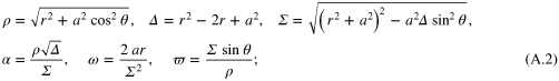
(ii) the 3 + 1 split of spacetime into space plus time embodied in this form of the metric; and (iii) the family of FIDOs whose world lines are orthogonal to the three-spaces of constant t, and their orthonormal basis vectors that lie in those three-spaces and are depicted in figure 1,

We shall also need three functions of r and of a ray's constants of motion b (axial angular momentum) and q (Carter constant), which appear in the ray's evolution equations (A.15) below—i.e., in the equations for a null geodesic:

And we shall need the function  , which identifies the constants of motion for rays (photons) that are unstably trapped in constant-r orbits around the black hole. This function is defined parametrically by [45]

where ro is the radius of the trapped orbit, which runs over the interval  , with

The prescription that we use, in DNGR, for computing the ray-tracing map and the blue shift is the following concrete embodiment of the discussion in section 2.1.
- (i)Specify the camera's location, and its speed β and the components , , and of its direction of motion relative to the FIDO at its location; and specify the ray's incoming direction on the camera's local sky. (Note: if the camera is in a circular, equatorial geodesic orbit around the black hole, thenis the geodesic angular velocity at the camera's radius rc, and the other quantities are defined in equations (A.2).)
- (ii)Compute, in the camera's proper reference frame, the Cartesian components (figure 1) of the unit vector that points in the direction of the incoming ray
- (iii)Using the equations for relativistic aberration, compute the direction of motion of the incoming ray,, as measured by the FIDO in Cartesian coordinates aligned with those of the camera:and from these, compute the components of on the FIDO's spherical orthonormal basis:
- (iv)Compute the ray's canonical momenta (covariant coordinate components of its four-momentum) with its conserved energy set to unity as a convenient convention: is the energy measured by the FIDO. (Note: can also be regarded as the ray's wave vector or simply as a tangent vector to the ray.) Then compute the ray's other two conserved quantities: its axial angular momentum b and its Carter constant q:(Note: if we had not set, then b would be and q would be (Carter constant).)
- (v)Determine, from the ray's constants, whether it comes from the horizon or the celestial sphere by the following algorithm: (a) Are both of the following conditions satisfied?: (v.1)with r1 and r2 given by equations (A.6) and the function given by equations (A.5); and (v.2) the ray's value of q lies in the range(b) If the answer to (a) is yes, then there are no radial turning points for that, whence if at the camera's location, the ray comes from the horizon; and if there, it comes from the celestial sphere. (c) If the answer to (a) is no, then there are two radial turning points for that , and if the camera radius rc is greater than or equal to the radius of the upper turning point, then the ray comes from the celestial sphere; otherwise, it comes from the horizon. Here is the largest real root of , with R(r) defined by equations (A.4).
- (vi)If the ray comes from the celestial sphere, then compute its point of origin there as follows: beginning with the computed values of the constants of motion and canonical momenta, and beginning in space at the camera's location, integrate the ray equations5numerically, backward in time from to , where is either or some very negative value. (This super-Hamiltonian version of the ray equations is well behaved and robust at turning points, by contrast, for example, with a commonly used version of the form , ,...; equations (33.32) of MTW [33].) The ray's source point on the celestial sphere is , .
- (vii)Compute the light's blue shift, i.e. the ratio of its frequency fc as seen by the camera to its frequency f' as seen by the source at rest on the celestial sphere, from


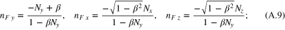


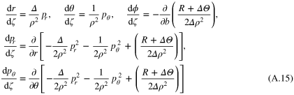


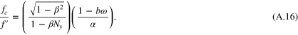
A.2. Ray-bundle equations
In this section we give a step-by-step prescription for evolving a tiny bundle of rays (a light beam) along a reference ray, from the camera to the celestial sphere, with the goal of learning the beam's major and minor angular diameters  and
and  on the celestial sphere, and the angle μ from
  on the celestial sphere to the beam's major axis (cf figure 1). As in the previous subsection, we set the black hole's mass to unity, M = 1.
Our prescription is a concrete embodiment of the discussion in section 2.2; it is a variant of the Sachs optical scalar equations [37]; and it is a slight modification of a prescription developed in the 1970s by Pineault and Roeder [35, 36]6 .
Our prescription relies on the following functions, which are defined along the reference ray. (a) The components of the ray bundle's four-momentum (wave vector) on the FIDO's orthonormal spherical basis
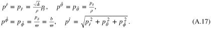
(b) A function  defined on the phase space of the reference ray by
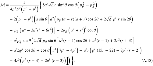
(c) A complex component  of the Weyl tensor, evaluated on vectors constructed from the ray's four-momentum; its real and imaginary parts work out to be:
Here Q1, Q2, w, and S are given by
We shall state our prescription for computing the shape and orientation of the ray bundle on the celestial sphere separately, for two cases: a ray bundle that begins circular at the camera; and one that begins elliptical. Then, we shall briefly sketch the Pineault–Roeder [35, 36] foundations for these prescriptions.
A.2.1. Circular ray bundle at camera
If the ray bundle begins at the camera with a tiny circular angular diameter  as measured by the camera, then our prescription for computing its shape and orientation at the celestial sphere is this:
- (i)Introduce five new functions along the reference ray:, , , , and (which are denoted x, y, p, q and χ by Pineault and Roeder). Give them and their derivatives the following initial conditions at the camera, :Here a dot means.
- (ii)Integrate the following differential equations backward along the ray toward its source at the celestial sphere, i.e. from to . These are coupled to the ray equations (A.15) for the reference ray.Here
- (iii)Upon reaching the celestial sphere at, evaluate the angular diameters of the bundle's major and minor axes using the equationsHere is the angular radius that the bundle would have had at the celestial sphere if spacetime curvature had not affected it:where the right-hand side is to be evaluated at the camera. Also evaluate the bundle's orientation angle at the celestial sphere fromwith the right-hand sides evaluated at the celestial sphere,, and with . The first term, χ, is the contribution from parallel transporting the bundle's major axis along the reference ray; the second term is the deviation from parallel transport caused by spacetime curvature.


A.2.2. Elliptical ray bundle at camera
Our prescription, for a ray bundle that begins elliptical at the camera, is this:
- (i)In the camera's proper reference frame, specify the Cartesian components of the bundle's major axis (a unit vector), subject to the constraint that be orthogonal to the ray direction (equation (A.8)), .
- (ii)Compute the major-axis direction in the FIDO frame using the transformation equationswhere β is the camera's speed (in the y direction) relative to the FIDO at its location.
- (iii)In the camera's reference frame, specify (a) the bundle's angular diameter along its major axis, and (b) the ratio e of the angular diameter along the minor axis to that along the major axis. These quantities are the same in the FIDO frame as in the camera frame: they are insensitive to special relativistic aberration.
- (iv)Then the initial conditions for the integration variables u, v, g, h, χ areHere is the Cartesian inner product, and and are two orthogonal unit vectors that span the plane orthogonal to the fiducial ray:
- (v)Continue and conclude with steps (ii) and (iii) of appendix A.2.1.


A.2.3. Foundations for these ray-bundle prescriptions
For completeness we briefly describe the Pineault–Roeder [35, 36] foundations for these ray-bundle-evolution prescriptions.
At an arbitrary location ζ along the reference ray, in the reference frame of a FIDO there, denote by  the components of the fiducial ray's unit tangent vector. (These are the same nF's as in the previous two subsections, extended to the fiducial ray's entire world line.) And at this arbitrary ζ, introduce the unit basis vectors
  and
and  (equations (A.30)) that span the plane orthogonal to the fiducial ray.
Notice that far from the black hole (at the celestial sphere), where  (negative because the reference ray is incoming),
  , the only nonzero components of these basis vectors are
  and
and  ; so
; so  and
and  .
.
We can think of the transverse plane at ζ as the complex plane, and think of the  direction as the real axis for complex numbers, and
  as the imaginary axis. Then any transverse vector
  can be represented by a complex number Y, with

To describe the ray bundle and its evolution, (following Pineault and Roeder) we introduce two complex numbers (transverse vectors) ξ and η, whose real and imaginary parts are functions that are evolved by the ray-bundle equations (A.23):

The outer edge of the ray bundle, at location ζ along the reference ray, is described by the complex number

where χ is also evolved by the ray-bundle equations. Here σ is a parameter that ranges from 0 to  , and as it changes, it carries the head of the vector
  around the bundle's edge. That vector, of course, is given by

(cf equation (A.31)), and its tail sits on the reference ray while its head sits on the edge of the bundle. One can verify that the shape of this  , with σ varying from 0 to
  , is an ellipse.
Let us denote by ν and λ the arguments of ξ and η, so  ,
,  . Then equation (A.33) reads
 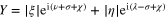 . As σ varies from 0 to
  , the modulus of Y (equal to the length of the vector
  ) reaches its largest value when the phase of the two terms is the same, i.e. when
  , or equivalently when
  . This maximal value of
  is
is

and the argument of Y at the max (the angle of  to
to  ) is
) is

The major diameter (not angular diameter) of the elliptical ray bundle, as measured by a FIDO at the location ζ, is this  multiplied by
  :
:

When the bundle reaches the celestial sphere, its measured angular diameter is the rate of increase of this major diameter with distance traveled. But at the celestial sphere, the distance traveled is equal to the affine parameter ζ, so the measured angular diameter is  . Now, the FIDO-measured light frequency fF is equal to f' at the celestial sphere, and the real and imaginary parts of
  and
and  are increasing linearly with ζ, so it turns out that the formula
  becomes the first of equations (A.25); and the angle μ of the major axis to the real axis
  , equation (A.36), becomes equation (A.27).
By an argument similar to the first part of the paragraph before last, one can deduce that anywhere along the evolving ray bundle

and correspondingly that the minor angular diameter at the celestial sphere is the second of equations (A.25).
The evolution equations (A.23) are the equation of geodesic deviation for the separation vector whose spatial part in a FIDO reference frame is the vector  (equation (A.34)) at fixed σ; see section II of Pineault and Roeder [36], and see [55].
A.3. Filtering
A.3.1. Spatial filtering and how we handle point stars
In DNGR we treat stars as point sources of light with infinitesimal angular size. We trace rays backwards from the camera to the celestial sphere. If we were to treat these rays as infinitely thin, there would be zero probability of any ray intersecting a star; so instead we construct a beam with a narrow but finite angular width, centred on a pixel on the camera's sky and extending over a small number of adjacent pixels, we evolve the shape of this beam along with the ray, and if the beam intercepts the star, we collect the star's light into it. This gives us some important benefits.
- The images of our unresolved stars remain small: they don't stretch when they get magnified by gravitational lensing.
- The fractional change in the beam's solid angle is directly related to the optical magnification due to gravitational lensing and hence to the intensity (brightness) change in the image of an unresolved star.
- When sampling images of accretion discs or extended structures such as interstellar dust clouds, we minimize moiré artefacts by adapting the resampling filter according to the shape of the beam [55].
Another consequence is that each star contributes intensity to several pixels. The eye is sensitive to the sum of these and as a single star crosses this grid, this sum can vary depending on the phase of the geometric image of the star on the grid7 . This can cause distracting flickering of stars as they traverse the virtual camera's image plane. We mitigate this effect by modulating the star's intensity across the beam with a truncated Gaussian filter and by setting the beam's initial radius to twice the pixel separation.
With this filter, the sum is brightest when the geometric image of the star falls exactly on a pixel and dimmest when centred between four pixels. The shape and width of the filter are designed to give a maximum 2% difference between these extremes, which we found, empirically, was not noticeable in fast changing Interstellar scenes.
This result assumes the final size of the ellipse is small and the shape of the beam does not change significantly between adjacent pixels. In extreme cases these assumptions can break down, leading to a distortion in the shape of a star's image, flickering, and aliasing artefacts. In these cases we can trace multiple beams per pixel and resample (see e.g. chapter 7 of [56]). However, Interstellar's black hole, Gargantua, when visualized, has a moderate spin  , which gives rise to few areas of extreme distortion, so we did not observe these problems in images created for the movie.
A.3.2. Temporal filtering: motion blur
For moving images, we need to filter over time as well as space. A traditional film camera typically exposes the film for half the time between individual frames of film, so for a typical 24 fps (frame per second) film, the exposure time will be 1/48 s. (This fraction is directly related to the camera's 'shutter angle': the shutters in film cameras are rotating discs with a slice cut out. The film is exposed when the slice is over the emulsion, and the film moves onto the next frame when covered. The most common shape is a semicircular disk which is a '180° shutter'.) Any movement of the object or camera during the exposure leads to motion blur. In our case, if the camera is orbiting a black hole, stellar images close to a critical curve appear to zip around in frantic arcs and would appear as streaks of light on a 1/48 s photograph. We aim to reproduce that effect when creating synthetic images for films.
This motion blur in computer graphics is typically simulated with Monte Carlo methods, computing multiple rays per pixel over the shutter duration. In order to cleanly depict these streaks with Monte Carlo methods, we would need to compute the paths of many additional rays and the computational cost of calculating each ray is very high. Instead, in DNGR we take an analytic approach to motion blur (cf figure A1 ) by calculating how the motion of the camera influences the motion of the deflected beam:

Figure A1. Left-to-right: no motion blur; Monte Carlo motion blur with four time samples per-pixel; analytic motion blur. Relative computation time is approximately in the ratio 1:4:2. Lens flare has been added to each image to illustrate how these images would typically be seen in the context of a movie.
Download figure:
Standard image High-resolution imageThe camera's instantaneous position influences the beam's momentary state, and likewise the camera's motion affects the time derivatives of the beam's state. We augment our ray and ray bundle equations (A.15) and (A.23) to track these derivatives throughout the beam's trajectory and end up with a description of an elliptical beam being swept through space during the exposure. The beam takes the form of a swept ellipse when it reaches the celestial sphere, and we integrate the contributions of all stars within this to create the motion-blurred image8 . These additional calculations approximately double the computation time, but this is considerably faster than a naive Monte Carlo implementation of comparable quality.
A.3.3. Formal description of our analytic approach to motion blur
We can put our analytic method into a more formal setting, using the mathematical description of motion blurred rendering of Sung et al [59], as follows. We introduce the quantity

which represents the resulting intensity of a sample located at coordinates (x, y) on the virtual image plane of the camera, corresponding to a ray direction ω, and subtending a solid angle, Ω. The sum is over each object, l, in the scene,  is the time the shutter is open, and
  represents the radiance of the object directed back toward the camera along ω from object l. The shutter and optics may filter the incident radiance (specific intensity) and this is accounted for by the term
  . The term
  is a geometric term that takes the value 1 if object l is visible or 0 if occluded.
Considering just the distortion of the celestial sphere to start with, we start with a ray in the direction  at time t0, in the middle of the exposure. We determine whether this ray gets swallowed up by the black hole or continues to the celestial sphere using equations (A.13) and (A.14). This corresponds to
  . We evolve the initial direction ω and solid angle Ω subtended by the sample into a new direction at the celestial sphere,
  , and ellipse
  , using the method described in appendices A.1 and A.2.
When the ray strikes the celestial sphere, we integrate over the area  , weighting the integration with our truncated Gaussian filter, corresponding to
  . (We assume there is no time-dependent aspect to this filter and ignore the t term. We also assume the celestial sphere is static.)
Our motion blur method approximates  with the following expression:
where the partial derivative is evaluated at the centre of the beam  and at t0. This represents a ray that can be swept over an arc in the celestial sphere by varying the value of t. This is convolved with the beam shape
  and filter and occlusion terms to give:
In this form, the consequences of our approximations become clearer: by evaluating g only at the beam centre  and shutter-centre t0, a sample that crosses the black hole's shadow during the exposure would be given a constant value of g (either 0 or 1) instead of the correct expression that transitions during the exposure. This would lead to a hard edge at the shadow if the camera performed a fast pan.
Luckily, in Interstellar, the design of the shots meant this rarely happened: the main source of motion blur was the movement of the spaceship around the black hole, and not local camera motion.
To handle any cases where this approximation might cause a problem, we also implemented a hybrid method where we launch a small number of Monte Carlo rays over the shutter duration and each ray sweeps a correspondingly shorter analytic path.
We used a very similar technique for the accretion disk.
A.4. Implementation
DNGR was written in C++ as a command-line application. It takes as input the camera's position, velocity, and field of view, as well as the black hole's location, mass and spin, plus details of any accretion disk, star maps and nebulae.
Each of the 23 million pixels in an IMAX image defines a beam that is evolved as described in appendix A.2.
The beam's evolution is described by the set of coupled first and second order differential equations (A.15) and (A.23) that we put into fully first order form and then numerically integrate backwards in time using a custom implementation of the Runge–Kutta–Fehlberg method (see, e.g., chapter 7 of [57]). This method gives an estimate of the truncation error at every integration step so we can adapt the step size during integration: we take small steps when the beam is bending sharply relative to our coordinates, and large steps when it is bending least. We use empirically determined tolerances to control this behaviour. Evolving the beam along with its central ray triples the time per integration step, on average, compared to evolving only the central ray.
The beam either travels near the black hole and then heads off to the celestial sphere; or it goes into the black hole and is never seen again; or it strikes the accretion disk, in which case it gets attenuated by the disk's optical thickness to extinction or continues through and beyond the disk to pick up additional data from other light sources, but with attenuated amplitude. We use automatic differentiation [58] to track the derivatives of the camera motion through the ray equations.
Each pixel can be calculated independently, so we run the calculations in parallel over multiple CPU cores and over multiple computers on our render-farm.
We use the OpenVDB library [60] to store and navigate volumetric data and Autodesk's Maya [61] to design the motion of the camera. (The motion is chosen to fit the film's narrative.) A custom plug-in running within Maya creates the command line parameters for each frame. These commands are queued up on our render-farm for off-line processing.
A.5. DNGR code characteristics and the Double Negative render-farm
A typical IMAX image has 23 million pixels, and for Interstellar we had to generate many thousand images, so DNGR had to be very efficient. It has 40 000 lines of C++ code and runs across Double Negative's Linux-based render-farm. Depending on the degree of gravitational lensing in an image9 , it typically takes from 30 min to several hours running on ten CPU cores to create a single IMAX image. The longest renders were those of the close-up accretion disk when we shoe-horned DNGR into Mantra. For Interstellar, render times were never a serious enough issue to influence shot composition or action.
Our London render-farm comprises 1633 Dell-M620 blade servers; each blade has two ten-core E5-2680 Intel Xeon CPUs with 156 GB RAM. During production of Interstellar, several hundred of these were typically being used by our DNGR code.
A.6. DNGR modelling of accretion disks
Our code DNGR includes three different implementations of an accretion disk.
Thin disk: for this, we adapted our DNGR ray-bundle code so it detects intersections of the beam with the disk. At each intersection, we sample the artist's image in the manner described in section 2.2 and appendix A.3 above, to determine the colour and intensity of the bundle's light and we attenuate the beam by the optical thickness (cf appendix A.4).
Volumetric disk: the volumetric accretion disk was built by an artist using SideFX Houdini software and stored in a volumetric data structure containing roughly 17 million voxels (a fairly typical number). Each voxel describes the optical density and colour of the disk in that region.
We used extinction-based sampling [62] to build a mipmap volume representation of this data. The length of the ray bundle was split into short piecewise-linear segments which, in turn, were traced through the voxels. We used the length of the major axis of the beam's cross section to select the closest two levels in the mipmap volume; and in each level we sampled the volume data at steps the length of a voxel, picking up contributions from the colour at each voxel and attenuating the beam by the optical thickness. The results from the two mipmap levels were interpolated before moving on to the next line segment.
Close-up disk with procedural textures: Side Effects Software's renderer, Mantra, has a plug-in architecture that lets you modify its operation. We embedded the DNGR ray-tracing code into a plug-in and used it to generate piecewise-linear ray segments which were evaluated through Mantra. This let us take advantage of Mantra's procedural textures10 and shading language to create a model of the accretion disk with much more detail than was possible with the limited resolution of a voxelized representation. However this method was much slower so was only used when absolutely necessary.
Disk layers close to the camera: the accretion-disk images in Interstellar were generated in layers that were blended together to form the final images. Occasionally a layer only occupied space in the immediate vicinity of the camera, so close that the infuences of spacetime curvature and gravitational redshifts were negligible. These nearby layers were rendered as if they were in flat spacetime, to reduce computation time.
Frequency shifts. in our visualizations that included Doppler and gravitational frequency shifts, we modelled the accretion disk as a constant-temperature blackbody emitter and we estimated the star temperatures from published NASA data [64]. The Doppler and gravitational frequency shifts correspond to a temperature shift in the blackbody spectra on arrival at the camera. We convolve those temperature-shifted black body spectra with the published spectral sensitivity curves of a typical motion picture film [63] to generate separate red, green and blue radiance values, R, G and B. For the volumetric disk, these are calculated at each step and used in place of artist-created radiance values. In figure 15(b) we removed the doppler-induced intensity change by dividing figure 15(d)'s RGB triplet of radiance values by a weighted mean that, empirically, leaves the eye-perceived colours unchanged:  . This dimmed the blue side of the disk and brightened the red side.
We set the white balance of our virtual camera to render a 6500 K blackbody spectrum with equal red, green and blue pixel values by applying a simple gain to each colour channel. We did not model the complex, nonlinear interaction between the colour-sensitive layers that occurs in real film.
A.7. Comparison of DNGR with astrophysical codes and with film-industry CGI codes
Near the end of section 1.1, we compared our code DNGR with the state-of-the-art astrophysical visualization code GRay. The most important differences—DNGR's use of light-beam mappings versus GRay's use of individual-ray mappings, and DNGR's use of ordinary processors versus GRay's use of GPUs—were motivated by our different goals: smoothness of images in movies versus fast throughput in astrophysics.
So far as we are aware, our code is unique in using light-beam-based mappings. No other code, astrophysical or film CGI, uses them. However, some film CGI codes use flat-spacetime mappings from the camera's image plane to the source plane that are mathematically equivalent to our light beams. Specifically, they use ray differential techniques described by Igehy [30], which track, along a ray, the transverse derivatives of the locations of nearby rays, thereby producing the matrix  , where
  is a ray's source-plane location as a function of its image-plane location. Tracking these differentials in flat spacetime is moderately easy because they are constant along straight paths between reflections, refractions, etc; and they change via simple matrix transformation laws at interaction locations. Tracking them through curved spacetime would entail the same geodesic-deviation technique as underlies our ray-bundle mappings.
In appendix A.3.1 we have described our methods of imaging star fields, using stars that are point sources of light: we feed each star's light into every light beam that intersects the star's location, with an appropriate weighting.
Other gravitational-lensing codes deal with star fields differently. For example, Müller and Frauendiener [29] calculate where each point-star ends up in the camera's image plane, effectively producing the inverse of the traditional ray-tracing algorithm. They do this for lensing by a non-spinning black hole (Schwarzchild metric) which has a high degree of symmetry, making this calculation tractable. Doing so for a spinning black hole would be much more challenging.
A common method for rendering a star-field is to create a 2D source picture (environment map) that records the stars' positions as finite-sized dots in the source plane (see e.g. [64]). This source picture is then sampled using the evolved rays from the camera. This has the disadvantage that stars can get stretched in an unrealistic way in areas of extreme magnification, such as near the critical curves described in section 3.3.1 of this paper. As we discussed in appendix A.3.1, our DNGR light-beam technique with point stars circumvents this problem—as does the Müller-Frauendiener technique with point stars.
Footnotes
- 3
We also have done such simulations but not in enough detail to reveal much new.
- 4
Our choice of Boyer–Lindquist coordinates prevents the camera from descending into the black hole. For that, it is not hard to switch to ingoing Kerr coordinates; but if one wants to descend even further, across an inner (Cauchy) horizon of the maximally extended Kerr spacetime, one must then switch again, e.g., to outgoing Kerr coordinates. Riazuelo [42] has created an implementation of the ray tracing equations that does such multiple switches. As a foundation for Interstellar, Thorne did so but only for the switch to ingoing Kerr coordinates, as Interstellar assumes the inner horizons have been replaced by the Marolf–Ori shock singularity [51] and the Poisson–Israel mass-inflation singularity [52]; see chapters 24 and 26 of [40].
- 5
- 6
The Pineault–Roeder equations (which were optimized for rays that begin near the black hole and travel from there to Earth) become asymptotically singular for our situation, where the rays begin on the celestial sphere and travel to a camera near the black hole. We have reworked the Pineault–Roeder analysis so as to make their equations fully nonsingular and robust for our situation. This reworking entailed changing their null vector
from to in equation (6) of [35]. This simple change of one foundational equation produced many changes in the final evolution equations for the ray bundle. Most importantly, it changed to in equations (A.19) and (A.21); the former diverges at the celestial sphere for our ingoing ray bundles, while the latter is finite there. For a detailed derivation of our prescription, see [55]. - 7
The same is true, of course, for each bit of a nebula or accretion disk. We discuss some details of how DNGR handles accretion disks in appendix A.6.
- 8
We took a similar approach when motion-blurring the accretion disks discussed in appendix A.6.
- 9
More specifically: the render time depends mainly on the number of steps in the integration. This, in turn, depends on the truncation errors in the integration scheme. The tolerances are tighter on the position of the ray than its shape, as errors in position give rise to more noticeable artefacts. Empirically, renders of regions close to the black hole's shadow are much slower than any other.
- 10
A procedural texture uses an algorithm, such as fractal noise, to generate detail at arbitrary resolution, unlike a texture based on an image file, which has a finite resolution.


