


ABSTRACT
We present measurements of the Hubble diagram for 103 Type Ia supernovae (SNe) with redshifts 0.04 < z < 0.42, discovered during the first season (Fall 2005) of the Sloan Digital Sky Survey-II (SDSS-II) Supernova Survey. These data fill in the redshift "desert" between low- and high-redshift SN Ia surveys. Within the framework of the mlcs2k2 light-curve fitting method, we use the SDSS-II SN sample to infer the mean reddening parameter for host galaxies, RV = 2.18 ± 0.14stat ± 0.48syst, and find that the intrinsic distribution of host-galaxy extinction is well fitted by an exponential function, P(AV) = exp(−AV/τV), with τV = 0.334 ± 0.088 mag. We combine the SDSS-II measurements with new distance estimates for published SN data from the ESSENCE survey, the Supernova Legacy Survey (SNLS), the Hubble Space Telescope (HST), and a compilation of Nearby SN Ia measurements. A new feature in our analysis is the use of detailed Monte Carlo simulations of all surveys to account for selection biases, including those from spectroscopic targeting. Combining the SN Hubble diagram with measurements of baryon acoustic oscillations from the SDSS Luminous Red Galaxy sample and with cosmic microwave background temperature anisotropy measurements from the Wilkinson Microwave Anisotropy Probe, we estimate the cosmological parameters w and ΩM, assuming a spatially flat cosmological model (FwCDM) with constant dark energy equation of state parameter, w. We also consider constraints upon ΩM and ΩΛ for a cosmological constant model (ΛCDM) with w = −1 and non-zero spatial curvature. For the FwCDM model and the combined sample of 288 SNe Ia, we find w = −0.76 ± 0.07(stat) ± 0.11(syst), ΩM = 0.307 ± 0.019(stat) ± 0.023(syst) using mlcs2k2 and w = −0.96 ± 0.06(stat) ± 0.12(syst), ΩM = 0.265 ± 0.016(stat) ± 0.025(syst) using the salt-ii fitter. We trace the discrepancy between these results to a difference in the rest-frame UV model combined with a different luminosity correction from color variations; these differences mostly affect the distance estimates for the SNLS and HST SNe. We present detailed discussions of systematic errors for both light-curve methods and find that they both show data-model discrepancies in rest-frame U band. For the salt-ii approach, we also see strong evidence for redshift-dependence of the color-luminosity parameter (β). Restricting the analysis to the 136 SNe Ia in the Nearby+SDSS-II samples, we find much better agreement between the two analysis methods but with larger uncertainties: w = −0.92 ± 0.13(stat)+0.10−0.33(syst) for mlcs2k2 and w = −0.92 ± 0.11(stat)+0.07−0.15 (syst) for salt-ii.
Export citation and abstract BibTeX RIS
1. INTRODUCTION
Ten years ago, measurements of the Hubble diagram of Type Ia supernovae (SNe) provided the first direct evidence for cosmic acceleration (Riess et al. 1998; Perlmutter et al. 1999). In the intervening decade, dedicated SN surveys have brought tremendous improvements in both the quantity and quality of SN Ia data, and SNe Ia remain the method of choice for precise relative distance determination over cosmological scales (e.g., Leibundgut 2001; Filippenko 2005). We now have in hand large, homogeneously selected samples of SNe Ia with relatively dense time-sampling in multiple passbands at redshifts z ≳ 0.3, most recently from the ESSENCE project (Miknaitis et al. 2007; Wood-Vasey et al. 2007) and the Supernova Legacy Survey (SNLS; Astier et al. 2006), augmented by smaller samples from the Hubble Space Telescope (HST) that extend to higher redshift (Garnavich et al. 1998; Knop et al. 2003; Riess et al. 2004, 2007). These data have confirmed and sharpened the evidence for accelerated expansion. Cosmic acceleration is most commonly attributed to a new energy-density component known as dark energy (for a review, see Frieman et al. 2008a). The recent SN measurements, in combination with measurements of the baryon acoustic oscillation (BAO) feature in galaxy clustering and of the cosmic microwave background (CMB) anisotropy, have provided increasingly precise constraints on the density, ΩDE, and equation of state parameter, w, of dark energy.
Despite these advances, a number of concerns remain about the robustness of current SN cosmology constraints. The SN Ia Hubble diagram is constructed from combining low- and high-redshift SN samples that have been observed with a variety of telescopes, instruments, and photometric passbands. Photometric offsets between these samples are highly degenerate with changes in cosmological parameters, and these offsets could be hidden in part because there is a gap or "redshift desert" between the low-redshift (z ≲ 0.1) SNe, found with small-aperture, wide-field telescopes, and the high-redshift (z ≳ 0.3) SNe discovered by large-aperture telescopes with relatively narrow fields. In addition, the low-redshift SN measurements that are used both to anchor the Hubble diagram and to train SN distance estimators were themselves compiled from combinations of several surveys using different telescopes, instruments, and selection criteria. Increasing the robustness of the cosmological results calls for larger SN samples with continuous redshift coverage of the Hubble diagram; it also necessitates high-quality data, with homogeneously selected, densely sampled, multi-band SN light curves and well-understood photometric calibration.
The Sloan Digital Sky Survey-II Supernova Survey (SDSS-II SN Survey; Frieman et al. 2008b), one of the three components of the SDSS-II project, was designed to address both the paucity of SN Ia data at intermediate redshifts and the systematic limitations of previous SN Ia samples, thereby leading to more robust constraints upon the properties of the dark energy. Over the course of three three-month seasons, the SDSS-II SN Survey discovered and measured well-sampled, multi-band light curves for roughly 500 spectroscopically confirmed SNe Ia in the redshift range 0.01 ≲ z ≲ 0.45. This data set fills in the redshift desert and for the first time includes both low- and high-redshift SN measurements in a single survey. The survey takes advantage of the extensive database of reference images, object catalogs, and photometric calibration previously obtained by the SDSS (for a description of the SDSS; see York et al. 2000).
In this paper, we present the Hubble diagram based on spectroscopically confirmed SNe Ia from the first full season (Fall 2005) of the SDSS-II SN Survey. To derive cosmological results, we include information from BAO (Eisenstein et al. 2005) and CMB measurements (Komatsu et al. 2009), and we also combine our data with our own analysis of public SN Ia data sets at lower and higher redshifts. We fit the SN Ia light curves with two models, mlcs2k2 (Jha et al. 2007) and salt-ii (Guy et al. 2007). We use the publicly available salt-ii software with minor modifications, but we have made a number of improvements to the implementation of the mlcs2k2 method, as described in Section 5.
Two companion papers explore related analyses with the same SN data sets. Lampeitl et al. (2009) combine the SDSS-II SN data with different BAO constraints and with measurements of redshift-space distortions and of the Integrated Sachs–Wolfe effect to derive joint constraints on dark energy from low-redshift (z < 0.4) measurements only; they also explore the consistency of the SN and BAO distance scales. Sollerman et al. (2009) use SN, BAO, and CMB measurements to constrain cosmological models with a time-varying dark energy equation of state parameter as well as more exotic models for cosmic acceleration. In all three papers, we use a consistent analysis of the SN data. Differences in cosmological inferences are attributable to differences in (1) the SN data included, (2) the other cosmological data sets included, and (3) the cosmological model space considered.
The outline of the paper is as follows. In Section 2, we briefly describe the operation and data processing for the SDSS-II SN Survey, which have been more extensively described in Sako et al. (2008). In Section 3, we summarize the spectroscopic analysis leading to final redshift and SN-type determinations (Zheng et al. 2008) and the photometric analysis leading to final SN flux measurements (Holtzman et al. 2008) for SDSS-II SNe. In Section 4, we present the SN samples and selection criteria applied to the light-curve data. We describe and compare the mlcs2k2 and salt-ii methods in Section 5. In Section 6, we describe detailed Monte Carlo simulations for the SDSS-II SN Survey and other SN data sets that we use to determine survey efficiencies and their dependences on SN luminosity, extinction, and redshift. Modeling of the survey efficiencies is needed to correct for selection biases that affect SN distance estimates. In Section 7, we use a larger spectroscopic+photometric SDSS-II SN sample to determine host-galaxy dust properties that are used in the mlcs2k2 fits. In particular, we present new measurements of the mean dust parameter, RV, and of the extinction (AV) distribution. In Section 8, we describe the cosmological likelihood analysis, which combines the SN Ia Hubble diagram with BAO and CMB measurements. In Section 9, we present a detailed study of systematic errors, showing how uncertainties in model parameters and in calibrations impact the results. In Section 10, we discuss the SN Hubble diagrams using the mlcs2k2 and salt-ii fitters and derive constraints on cosmological parameters. We provide a detailed comparison of the mlcs2k2 and salt-ii results in Section 11, and we conclude in Section 12. Appendices provide details on the methods for warping the SN Ia spectral template for K-corrections, modeling the filter passbands for the Nearby SN Ia sample, determining the magnitudes of the primary photometric standard stars, extracting the distribution of host-galaxy dust extinction from the SDSS-II sample, and estimating error contours that include systematic uncertainties. They also include discussion of the scatter in the SDSS-II Hubble diagram and of the translation of the salt-ii model into the mlcs2k2 framework.
2. SDSS-II SUPERNOVA SURVEY
The scientific goals, operation, and basic data processing for the SDSS-II SN Survey are described in Frieman et al. (2008b), and details of the SN search algorithms and spectroscopic observations are given in Sako et al. (2008). Here we provide a brief summary of the Fall 2005 campaign, in order to set the context for the data analysis.
The SDSS-II SN Survey primary instrument was the SDSS CCD camera (Gunn et al. 1998) mounted on a dedicated 2.5 m telescope (Gunn et al. 2006) at Apache Point Observatory (APO), New Mexico. The camera obtains, nearly simultaneously, images in five broad optical bands: ugriz (Fukugita et al. 1996). The camera was used in the time-delay-and-integrate (TDI, or drift scan) mode, which provides efficient sky coverage. The SN Survey scanned at the normal (sidereal) SDSS survey rate, which yielded 55 s integrated exposures in each passband; the instrument covered the sky at a rate of approximately 20 deg2 hr−1.
On most of the usable observing nights in the period 1 September through 2005 November 30, the SDSS-II SN Survey scanned a region (designated stripe 82) centered on the celestial equator in the Southern Galactic Hemisphere that is 2 5 wide and runs between right ascensions of 20hr and 4hr, covering a total area of 300 deg2. Due to gaps between the CCD columns, on a given night slightly more than half of the declination range of the stripe was imaged; on succeeding nights, the survey alternated between the northern (N) and southern (S) declination strips of stripe 82 (see Stoughton et al. 2002 for a description of the SDSS observing geometry). Accounting for CCD gaps, bad weather, nearly full Moon, and other observing programs, a given region was imaged on average every four to five nights under a variety of conditions. This relatively high cadence enabled us to obtain well-sampled light curves, typically starting well before peak light.
At the end of each night of imaging, the SN data were processed using a dedicated 20-CPU computing cluster at APO. Images were processed through the PHOTO photometric reduction pipeline to produce corrected u, g, r, i, z frames (Lupton et al. 2001; Ivezić et al. 2004), each with an astrometric solution (Pier et al. 2003), point-spread-function (PSF) map, and zero point. A co-added template image, consisting of typically eight stacked images taken in previous years, was matched to the new image and subtracted from it. Subtracted gri images were searched for pixel clusters with an excess flux (roughly 3σ) above the noise in the subtracted image, and a position and total PSF flux were assigned for each significant detection. We positionally matched detections in multiple passbands: objects are detections in at least two of the three gri passbands with a displacement of less than 0 8 between detections in each filter. This displacement cut was chosen to ensure high efficiency for objects with low signal to noise. The g and r exposures of a given object were taken five minutes apart, enabling many fast asteroids to be removed by the 08 requirement. Finally, a catalog of 105 previously detected variables (mainly stars and active galactic nuclei (AGNs)) and 4 million stars (r < 21.5) was used to reject detections within 1'' of any object in the catalog; nearly 40,000 such detections were automatically vetoed during the Fall 2005 survey.
During the season, 20'' × 20'' cutouts of the resulting ∼140, 000 object images were visually scanned by humans,38 typically within 24 hr of when the data were obtained. The human scanning was done to eliminate objects that were clearly not SNe, such as unsubtracted diffraction spikes, other subtraction artifacts, and obvious asteroids. To monitor the software pipelines and human scanning efficiency, "fake" SNe were inserted on top of galaxies in the images during processing. Approximately 11,400 of the objects were tagged by a scanner as a possible SN candidate. Nearly 60% of the candidates appeared only once during the survey; most of these are likely slow-moving solar system objects. After a night of observations, each candidate light curve (in g, r, i) was updated and compared with a set of SN light-curve templates that include SNe Ia as a function of redshift, intrinsic luminosity, and extinction, as well as non-Ia SN types. Light curves that matched best to an SN Ia template (at any reasonable redshift, luminosity, and extinction) were preferentially scheduled for spectroscopic follow-up observations. Candidates with r-band magnitude r ≲ 20.5 were given highest priority for follow-up, regardless of photometric SN type; for SNe Ia, this magnitude cut corresponds roughly to redshifts z < 0.15. For fainter SN Ia candidates, spectroscopic priority was given to candidates with the best chance of acquiring a useful spectrum. In order of importance, the prioritization criteria were: (1) SN is well-separated (≳1'') from the core of its host galaxy, (2) reasonable SN/galaxy brightness contrast based on visual inspection, and (3) SN host galaxy is relatively red (early-type). In most cases, a detection in at least two epochs was required before a spectrum was obtained.
Spectra of SN candidates and, where possible, their host galaxies were obtained in 2005 September–December with a number of telescopes (Frieman et al. 2008b; Zheng et al. 2008): the Hobby-Eberly 9.2 m at McDonald Observatory, the Astrophysical Research Consortium 3.5-meter at APO, the Subaru 8.2-meter on Mauna Kea, the Hiltner 2.4 m at MDM Observatory, the 4.2 m William Herschel Telescope on La Palma, and the Keck 10 m on Mauna Kea. Approximately 90% of the SN Ia candidates that were spectroscopically observed were confirmed as SNe Ia.
As noted below (Section 3.1), 146 spectroscopically observed candidates from 2005 were classified as definitive or possible SNe Ia based on analysis of their spectra. For these candidates, there are a total of more than 2000 photometric epochs, where each epoch corresponds to a measurement (not necessarily a detection) in the ugriz passbands within a time window of −15 days to +60 days relative to peak brightness in the SN rest-frame. About half of the epochs were recorded in "photometric" conditions, defined as no moon, PSF less than 17, and no clouds as indicated by the SDSS cloud camera, which monitors the sky at 10 μm (Hogg et al. 2001). Another 30% of the measurements were recorded in non-photometric (but moonless) conditions. The remaining 20% of the measurements were taken with the moon above the horizon.
3. SDSS SN SPECTROSCOPIC AND PHOTOMETRIC REDUCTION
For each SN candidate found during the survey, the on-mountain software pipeline described in Section 2 delivered preliminary photometric measurements. Similarly, spectroscopic observations were reduced in near-real time so that estimates of SN type and redshift could be made. Although these initial measurements were sufficient for discovering and confirming SNe, for the final analysis and sample selection we require more accurate photometry (Holtzman et al. 2008) and a more uniform spectroscopic analysis (Zheng et al. 2008). This section briefly describes these techniques.
3.1. Supernova Typing and Redshift Determination
After the finish of the Fall 2005 season, all of the SN spectra were processed with IRAF (Tody 1993). Classification of the reduced SN spectra was aided by the IRAF package rvsao.xcsao (Tonry & Davis 1979), which cross-correlates the spectra with libraries of SN spectral templates and searches for significant peaks. Details of this analysis are described in Zheng et al. (2008). About half of the SN spectra had an excellent template match, while the other half required more human judgment for the SN typing. Based on this analysis, 130 candidates were classified as confirmed SNe Ia and 16 candidates were classified as probable SNe Ia.
For 29 of these 146 candidates, we have used the SDSS host-galaxy spectroscopic redshift as reported in the SDSS DR4 database; typical redshift uncertainties are 1–2 ×10⁻⁴. For SN 2005hj, a host-galaxy spectroscopic redshift and its uncertainty were obtained by Quimby et al. (2007). For 82 of the candidates that do not have a host spectroscopic redshift in the DR4 database, we use the redshift from host-galaxy spectral features obtained with our own spectroscopic observations. The redshift precision in those cases is estimated to be 0.0005, the rms difference between our host-galaxy redshifts and those measured by the SDSS spectroscopic survey (DR4) for a sample in which both redshifts are available. For the remaining 34 candidates, our redshift estimate is based on spectroscopic features of the SNe, with an estimated uncertainty of 0.005, the rms spread between the SN redshifts and host-galaxy redshifts. In summary, 77% of the spectroscopically confirmed and probable SNe Ia have spectroscopic redshifts determined from host-galaxy features, while the rest have redshifts based on SN spectral features. The redshifts are determined in the heliocentric frame and then transformed to the CMB frame as described in Section 8.
The redshift distribution for the 130 confirmed SNe Ia from the 2005 season is shown below in Figure 2(e). The relative deficit of confirmed SNe at redshifts between 0.15 and 0.25 is due to the finite spectroscopic resources that were available for the Fall 2005 campaign and to the relative priorities given to low- and high-redshift candidates for the different telescopes (Sako et al. 2008). Subsequently, host-galaxy redshifts have been obtained for most of the "missing" SN Ia candidates with SN Ia like light curves in this redshift range. These photometrically identified (but spectroscopically unconfirmed) candidates with host-galaxy redshifts are used in the determination of host-galaxy dust properties (Section 7), but we do not include them in the Hubble diagram for this analysis. Compared to the Fall 2005 season, spectroscopic observations during the 2006 and 2007 seasons were more complete around redshifts z ∼ 0.2.
3.2. Supernova Photometry
To achieve precise and reliable SN photometry, we developed a new technique called "Scene Model Photometry" (SMP) that optimizes the determination of SN and host–galaxy fluxes. This method and the Fall 2005 SN photometry results are described in detail in Holtzman et al. (2008).
The basic approach of SMP is to simultaneously model the ensemble of survey images covering an SN location as a time-varying point source (the SN) and sky background plus time-independent galaxy background and nearby calibration stars, all convolved with a time-varying PSF. The calibration stars are taken from the SDSS catalog for stripe 82 produced by Ivezić et al. (2007). The fitted parameters are SN position, SN flux for each epoch and passband, and the host host-galaxy intensity distribution in each passband. The galaxy model for each passband is a 20 × 20 grid (with a grid scale set by the CCD pixel scale, 04 × 04) in sky coordinates, and each of the 400 × 5 = 2000 galaxy intensities is an independent fit parameter. As there is no pixel re-sampling or image convolution, the procedure yields correct statistical error estimates. Holtzman et al. (2008) describes the rigorous tests that were carried out to validate the accuracy of SMP photometry and of the error estimates.
Although we have obtained additional imaging on other telescopes for a subsample of the confirmed SNe Ia, only photometry from the SDSS 2.5 m telescope is used in this analysis. Figure 1 shows four representative SDSS-II SN Ia light curves processed through SMP and provides an indication of the typical sampling cadence and signal to noise as a function of redshift.
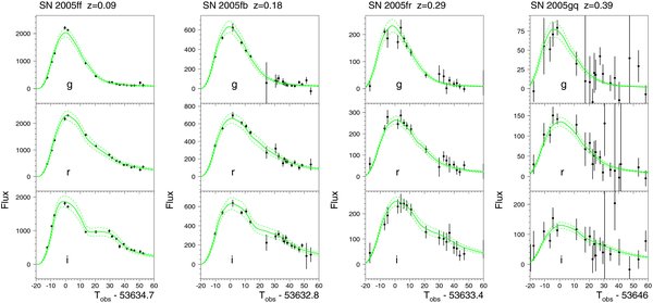
Figure 1. Light curves for four SDSS-II SNe Ia at different redshifts: SN 2005ff at z = 0.09, SN 2005fb at z = 0.18, SN 2005fr at z = 0.29, and SN 2005gq at z = 0.39. The passbands are SDSS g (top), r (middle), and i (bottom). Points are the SMP flux measurements (flux = 10(11 − 0.4m), where m is the SN magnitude) with ±1σ photometric errors indicated. Solid curves show the best-fit mlcs2k2 model fits (see Section 5.1), and dashed curves give the ±1σ error bands on the model fits. The Modified Julian Date (MJD) under each set of light curves is the fitted time of peak brightness for the rest-frame B band.
Download figure:
Standard image High-resolution imageThe fluxes and magnitudes returned by SMP are in the native SDSS system (Ivezić et al. 2007). The SDSS photometric system is nominally on the AB system, but the native flux in each filter differs from that of a true AB system by a small amount. AB magnitudes are obtained by adding the AB offsets in Table 1 to the native magnitudes. The offsets are determined by comparing photometric measurements of the HST standard solar analogs P3330E, P177D, and P041C with synthetic magnitudes based on the published HST spectra (Bohlin 2007) and SDSS filter bandpasses. Since the standard stars are too bright to be measured directly with the SDSS 2.5 m telescope, the measurements are taken with the 0.5 m SDSS Photometric Telescope (the PT) and transformed to the native system of the SDSS telescope. The technique of transferring the PT magnitudes to the native SDSS system is identical to that used to obtain the SDSS photometric calibration (Tucker et al. 2006). The uncertainty in the AB offsets is estimated to be 0.003, 0.004, 0.004, 0.007, 0.010 mag (for u, g, r, i, z) based on the internal consistency of the three standard solar analogs. The uncertainties given in Table 1 are larger, since they also account for the ∼10 Å uncertainties in the central wavelengths (given in the same table) of the SDSS filters.
Table 1. AB Offsets and Central Wavelength Uncertainties for the SDSS Filters
| SDSS Filter | AB Offset (mag) and Its Uncertaintya | Uncertainty (Å) on Central Wavelength |
|---|---|---|
| u | −0.037 ± 0.014 | 8 |
| g | +0.024 ± 0.009 | 7 |
| r | +0.005 ± 0.009 | 16 |
| i | +0.018 ± 0.009 | 25 |
| z | +0.016 ± 0.010 | 38 |
Note. aErrors account for uncertainties in the central wavelengths of the SDSS filters.
Download table as: ASCIITypeset image
4. SUPERNOVA SAMPLE SELECTION
In this section, we describe the light-curve selection criteria used to define the SN Ia samples. To minimize systematic errors associated with analysis methods and assumptions, we perform a nearly uniform analysis on data from SDSS-II, the published data from ESSENCE (Wood-Vasey et al. 2007; hereafter WV07), SNLS (Astier et al. 2006), HST (Riess et al. 2007), and a Nearby SN Ia sample collected over a decade from several surveys and a number of telescopes (Jha et al. 2007; hereafter JRK07). Although these data samples are analyzed in a homogeneous fashion, we present more details about the SDSS-II analysis since these data are presented here for the first time and, more importantly, because we use the SDSS-II sample in Section 7 to make inferences about the SN Ia population that we apply to all the data samples.
Light curves with good time sampling and good signal to noise are needed to yield reliable distance estimates. We therefore apply stringent selection cuts to all five photometric data samples used in this analysis. The cuts are also chosen to define samples whose selection functions can be reliably modeled with the Monte Carlo simulations described in Section 6. In future analyses the cuts will be further refined based on studies with simulated samples.
We first present the selection cuts we have applied and then briefly discuss the rationale for each of them. Defining Trest as the rest-frame time, such that Trest = 0 corresponds to peak brightness in rest-frame B band according to mlcs2k2, we select for inclusion in the cosmology analysis SN Ia light curves that satisfy the following criteria.
- 1.For SDSS-II, ESSENCE, SNLS, and HST, at least one measurement is required before peak brightness (Trest < 0 days); for the Nearby sample, at least one measurement is required with Trest < +5 days. The requirement on the Nearby sample is relaxed, because nearly half the sample would be rejected by the more stringent cut of Trest < 0 days.
- 2.At least one measurement with Trest > + 10 days.
- 3.At least five measurements with −15 < Trest < +60 days.
- 4.At least one measurement with signal-to-noise ratio (S/N) above 5 for: each of SDSS g, r, and i; both SNLS r and i (no requirement on g, z); HST F814W_WFPC2 and at least one other HST passband. For the ESSENCE sample, we adopt the cuts from WV07: at least one measurement at Trest < +4 days that has S/N >5, at least one measurement at Trest > + 9 days that has S/N >5, and at least eight total measurements with S/N >5. Since the Nearby SN Ia sample includes only events with high S/N, no S/N requirement is needed for that sample.
- 5.
 , where is the mlcs2k2 light-curve fit probability based on the χ2 per degree of freedom (see Section 5.1).
 - 6.z > zmin = 0.02, which only affects the Nearby SN Ia sample.


For all the data samples we only include unambiguous spectroscopically confirmed SNe Ia; in particular, for the SDSS-II sample, we do not include the 16 spectroscopically probable SNe Ia (see Section 3.1). Moreover, for the SDSS-II sample, we use only g, r, i photometry in the analysis, and we reject ∼4% of the epochs for which the SMP pipeline (Section 3.2) did not return a reliable flux estimate.
For the first three requirements in the list above, a "measurement" corresponds to a recorded photometric measurement in a single passband and can have any signal-to-noise value, i.e., a significant detection is not necessary. These requirements collectively ensure that the time sampling of the light curve is sufficient to yield a robust light-curve model fit, with coverage before and after peak light so that the epoch of peak light can be reliably estimated. To illustrate the motivation for requiring a measurement before peak light (which was not explicitly required in either the Astier et al. (2006) or WV07 analyses), consider SN g133 in the ESSENCE sample, which has no measurements before peak and is therefore rejected in our analysis. Compared to the published values in WV07, our mlcs2k2 fitted time of maximum brightness is 10 days earlier, and our fitted distance modulus is 0.4 mag smaller. The fourth requirement, on S/N, similarly puts a floor on the quality of the light-curve data. The fifth requirement, on mlcs2k2 light-curve fit probability  , is designed to remove obviously peculiar SNe in an objective fashion. This cut removes the previously identified peculiar SNe Ia in the SDSS-II sample, 2005hk (Phillips et al. 2007; Chornock et al. 2006), 2005gj (Aldering et al. 2006; Prieto et al. 2007), and SDSS-II SN 7017 (which is similar to 2005gj). In the Nearby sample, it rejects the following peculiar SNe: 1992bg, 1995bd, 1998de, 1999aa, 1999gd, 2001ay, 2001bt, 2002bf, and 2002cx.
The sixth selection criterion, corresponding to czmin = 6000 km s−1, removes objects from the Nearby sample for which the typical galaxy peculiar velocity, vpec ∼ 300 km s−1, is a non-negligible fraction of the Hubble recession velocity. In principle, this cut on redshift could be replaced by a redshift- and position-dependent weighting covariance factor that includes the effects of both random and correlated peculiar velocities (Hui & Greene 2006; Cooray & Caldwell 2006). In this analysis, we follow recent practice and simply impose a lower redshift bound, but this approach raises the issue of how to select zmin. Astier et al. (2006) and WV07 used zmin = 0.015. However, using mlcs2k2, JRK07 found that the Hubble parameter inferred from the lowest-redshift SNe, with z ≲ 0.025, is systematically higher than that obtained using more distant (0.025 < z < 0.1) Nearby SNe, consistent with an earlier result of Zehavi et al. (1998). JRK07 also noted that varying zmin from 0.008 to 0.027 changes the dark energy equation of state by δw ∼ 0.2 for the Nearby SN Ia sample in combination with a simulated ESSENCE sample. As a consequence, Riess et al. (2004, 2007) used zmin = 0.023 (czmin = 7000 km s−1), i.e., they only included SNe beyond the so-called Hubble bubble. On the other hand, Conley et al. (2007) found that the Hubble bubble is not significant when the salt-ii fitter is used. As discussed in Section 9.1, we find that the best-fit value of w is sensitive to the choice of zmin whether we use mlcs2k2 or salt-ii. Varying zmin, we find that zmin = 0.02 corresponds to the middle of the range of w variations for the mlcs2k2 method. For the salt-ii method, w varies rapidly with zmin near zmin ∼ 0.015, and is more stable when zmin ≳ 0.02. On this basis, we choose zmin = 0.02 for both light-curve fitting methods and include the effects of varying zmin in the systematic-error budget.
For the SDSS-II sample of 130 spectroscopically confirmed SNe Ia from the Fall 2005 season, 103 satisfy these selection criteria. The cut-rejection statistics are as follows: 3 are photometrically peculiar SNe Ia that fail the  requirement; 9 have no measurement before peak brightness—most of these were discovered early in the survey season; 11 have no measurement with Trest > + 10 days—most of these were discovered late in the survey season or were at the high-redshift end of the distribution; and 4 SNe Ia in the high-redshift tail, z ∼ 0.4, fail the S/N requirement.
With the selection criteria defined above, the number of SN Ia events used for fitting is shown in Table 2 for each sample; a total of 288 SNe Ia are included in the fiducial analysis (in systematic-error tests, e.g., varying zmin, this number fluctuates by a small amount). Table 2 also shows the average number of measurements per SN Ia for each sample, where a measurement is an observation in a single passband in the rest-frame time interval −15 to +60 days. The average number of measurements is about 50 for both the Nearby and SDSS-II samples, in the twenties for ESSENCE and SNLS, and 11 for HST. We note that our selection requirements are more restrictive than those applied in previous analyses. WV07 included 60 out of 105 spectroscopically confirmed ESSENCE SNe Ia for their mlcs2k2 analysis,39 while our cuts select 56. WV07 selected 45 SNe Ia from the Nearby sample (z > 0.015), while we include 33 (z > 0.02); the difference is mainly due to the different redshift cuts. Astier et al. (2006) included 71 SNLS SNe Ia, while we retain 62 from the same sample.
Table 2. Redshift Range, Number of SNe Passing Selection Cuts, and Mean Number of Measurements for Each SN Sample
| Sample (Obs Passbands) | Redshift Range | NSNa | 〈Nmeas〉b |
|---|---|---|---|
| Nearby (UBVRI) | 0.02–0.10 | 33 | 52 |
| SDSS-II (gri) | 0.04–0.42 | 103 | 48 |
| ESSENCE (RI) | 0.16–0.69 | 56 | 21 |
| SNLS (griz) | 0.25–1.01 | 62 | 27 |
| HST (F110W, F160W, | 0.21–1.55 | 34 | 11 |
| F606W, F775W, F850LP) |
Notes. aNumber of SNe Ia passing cuts. bAverage number of measurements per SN Ia, in the interval −15 < Trest < +60 days.
Download table as: ASCIITypeset image
Figure 2 shows distributions in the SDSS-II sample—before selection cuts—for some of the variables used in sample selection, as well as the SDSS-II SN Ia redshift distribution before and after selection cuts are applied. Figure 3 shows the redshift distribution for all five samples, along with the average of the maximum observed S/N as a function of redshift.
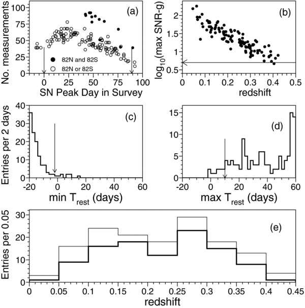
Figure 2. For the spectroscopically confirmed SN Ia sample from the SDSS-II 2005 season, distributions are shown for (a) number of gri measurements with −15 < Trest < +60 days as a function of day in the survey season when the SN reached peak luminosity. Vertical arrows show the start (September 1) and end dates (November 30) of the survey season. SNe that lie in the overlap region of strips 82N and 82S (solid dots) tend to have more measurements; (b) log10 of maximum g-band S/N vs. redshift; (c) time of first measurement relative to peak light in rest-frame B; (d) time of last measurement (not necessarily detection) relative to peak light—the pile-up near 60 days is from SNe that have measurements past 60 days; (e) redshifts before (130, thin line) and after (103, thick line) selection cuts are applied. The arrows in panels (b), (c), and (d) indicate the selection cuts.
Download figure:
Standard image High-resolution image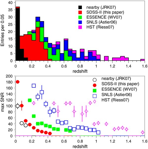
Figure 3. Top panel: summed redshift distribution for the five SN Ia samples indicated in the legend. Bottom panel: maximum observed S/N (among all passbands) as a function of redshift, averaged in bins of width Δz = 0.05; error bars indicate the rms spread within each bin. All selection requirements have been applied.
Download figure:
Standard image High-resolution image5. LIGHT-CURVE ANALYSIS
In this section, we describe our methods of analyzing SN light curves and extracting distance estimates. The two light-curve fitting methods we employ, mlcs2k2 and salt-ii, reflect different assumptions about the nature of color variations in SNe Ia, different approaches to training the models using pre-existing data, and different ways of determining model parameters.
5.1. mlcs2k2 Fitting Method
The Multicolor Light-Curve Shape method, known as mlcs2k2 in its current incarnation (JRK07), has been in use for more than a decade; the original MLCS version (Riess et al. 1998) was used by the High-z Supernova Team in the discovery of cosmic acceleration. For each SN, mlcs2k2 returns an estimated distance modulus and its uncertainty; the redshift and distance modulus for each SN are inputs to the cosmology fit discussed in Section 8.
mlcs2k2 describes the variation among SN Ia light curves with a single parameter (Δ). Excess color variations relative to the one-parameter model are assumed to be the result of extinction by dust in the host galaxy and in the Milky way. The mlcs2k2 model magnitude is given by
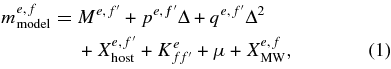
where e is an epoch index that runs over the observations, f are observer-frame filter indices, f' = UBVRI are the rest-frame filters for which the model is defined, Δ is the mlcs2k2 shape-luminosity parameter that accounts for the correlation between peak luminosity and the shape/duration of the light curve, Xhost is the host-galaxy extinction, XMW is the Milky Way extinction,  is the K-correction between rest-frame and observer-frame filters, and μ is the distance modulus, which satisfies μ = 5log10(dL/10pc), where dL is the luminosity distance. We use this model for SN epochs in the rest-frame time range −15 < Trest < +60 days relative to rest-frame B–maximum. Observer-frame passbands are included that satisfy
  Å, where
  is the mean wavelength of the filter passband, and z is the redshift of the SN Ia. To account for larger model uncertainties in the rest-frame UV region, a K-correction uncertainty of
  mag is added in quadrature to the model error for
  Å.
Å.
In the mlcs2k2 model, the shape-luminosity parameter Δ describes the intrinsic SN color dependence on brightness, and Xhost describes SN color variations from reddening (extinction) by dust in the host galaxy, which is assumed to behave in a manner similar to dust in the Milky Way. In particular, the extinction is described by the parameterization of Cardelli et al. (1989) (hereafter CCM89),  , where AV is the extinction in magnitudes in the V band, aV = 1, bV = 0, and the relative extinction in other passbands is determined by the parameter RV, the ratio of V-band extinction to color excess, RV = AV/E(B − V). For the Milky Way, the value of RV averaged over a number of lines of sight is RV = 3.1; this global value has been adopted in previous SN analyses using mlcs2k2. For the galaxies that host SNe Ia, we instead adopt RV = 2.18 ± 0.50, as derived in Section 7.2 from the SDSS-II SN data.
The coefficients  ,
,  , and
, and  are model vectors that have been evaluated using nearly 100 well-observed low-redshift SNe as a training set.
  is the absolute magnitude for an SN Ia with Δ = 0. Assuming a Hubble parameter h = H0/100 km s−1 Mpc−1 = 0.65, the resulting absolute magnitudes at peak brightness are −20.00, −19.54, −19.46, −19.45, −19.18 mag for U, B, V, R, I, respectively. The p and q vectors translate the shape-luminosity parameter Δ into a change in the SN Ia absolute magnitude. The
  values (at peak brightness) vary among passbands from 0.6 to 0.8, and the
  vary from 0.1 to 0.9; therefore, intrinsically faint (bright) SNe have positive (negative) values of Δ.
We use model vectors based on the procedure outlined in JRK07, but with two notable differences. First, the vectors have been re-evaluated based on our determination of the dust parameter, RV = 2.18. Since most of the nearby objects used in the training have low extinction, retraining with a different value of RV has little effect on the vectors and therefore on the cosmological results. Note that the insensitivity of the mlcs2k2 training to the value of RV does not imply that the estimated distances for high-redshift SNe are insensitive to the value of RV, especially since the latter samples include highly extinguished SNe. The impact of RV on the cosmology results is presented in Section 9.
The second change in the model vectors from JRK07 involves adjustments to the  that were developed during the course of the WV07 analysis of the ESSENCE data. For the model training with the Nearby SN Ia sample, it was assumed that the observed AV distribution has the functional form of an exponential distribution convolved with a Gaussian centered at AV = 0. However, the mlcs2k2 training process resulted in a convolution Gaussian that is not centered at zero; adjustments were made in the vectors such that the Gaussian is centered at zero. The main caveat in this procedure is that the selection efficiency for the Nearby sample is small and unknown, and therefore it is not straightforward to model the observed AV distribution in terms of an underlying population. The
  adjustments for UBVRI depend only on the passband and are independent of epoch. For the model vectors determined with RV = 2.2, the magnitude adjustments relative to the values in JRK07 are

K-corrections transform the mlcs2k2 SN rest-frame Landolt-system magnitudes to the magnitudes of a redshifted SN in an observed passband. K-corrections are computed following the prescription of Nugent et al. (2002), which requires an SN spectrum at each epoch, the spectrum of a reference star, and the reference star magnitude in each passband. As explained in Appendix A, we use a single template spectrum for each SN epoch and warp it to match the colors of the SN model. Since the Landolt photometry is not associated with a precisely defined set of filters, we use the standard UBVRI and BX filters defined by Bessell (1990) and apply a color transformation to obtain photometry in the Landolt system. That procedure is detailed in Appendix B. In place of the traditional primary reference star Vega, we choose BD+17°4708 (Oke & Gunn 1983) as our primary reference because it has been measured by Landolt, it has a precise HST STIS spectrum (Bohlin 2007) and it is the primary reference for SDSS photometry. We have also carried out the analysis with Vega as the primary reference and include the difference as a systematic error. The primary magnitudes for each filter system are given in Table 22 of Appendix C for both BD+17 and Vega.
A light-curve fit determines the likelihood function  of the observed magnitudes or fluxes as a function of four model parameters for each SN Ia: (i) time of peak luminosity in rest-frame B band, t0, (ii) shape-luminosity parameter, Δ, (iii) host-galaxy extinction at central wavelength of rest-frame V band, AV, and (iv) the distance modulus, μ. The redshift (z) is accurately determined from the spectroscopic analysis, so it is not included as a fit parameter; the redshift uncertainty is included in the cosmology analysis (Section 8). For each SN, the log of the posterior probability Ppost, or χ2 statistic, is given by
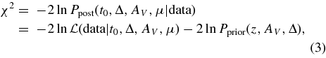
where Pprior is a Bayesian prior (see below), and the log-likelihood is given by
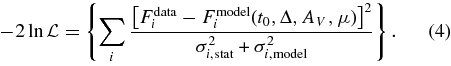
Here the index i runs over all measured epochs and observer-frame passbands, and Fdatai is the observed flux for measurement i. The statistical measurement uncertainty, σstat, is estimated from the SMP as described in Section 3.2. For the model uncertainty, σmodel, we use the diagonal elements of the mlcs2k2 covariance matrix, which are estimated from the spread in the training sample of SNe. For example, at the epoch of peak brightness (t0) these model errors are 0.11, 0.07, 0.08, 0.10, 0.11 mag for U, B, V, R, I, respectively; the uncertainties increase monotonically with time away from t0. As explained below in the list of modifications, we do not use the off-diagonal mlcs2k2 correlations in this analysis.
Since AV is a physical parameter that is always positive, and since it is not well constrained if peak S/N is low or if the observations do not span a large wavelength range, the mlcs2k2 fit includes a Bayesian prior on the extinction. The prior forbids negative values of AV and encodes information about the distribution of extinction in SN host galaxies as well as the selection efficiency of the survey. Since there is degeneracy between the inferred values of AV and μ, the prior leads to reduced scatter in the Hubble diagram. For the Nearby SN sample, which has high peak S/N for all objects, the prior has no impact on the Hubble scatter; for the other samples we employ, the prior reduces the Hubble scatter by a factor of 1.3–2. For this analysis, the prior is defined to be
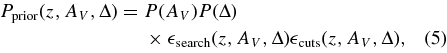
where P(AV) and P(Δ) are the underlying SN Ia population distributions of AV and Δ, and we assume that these distributions are independent of redshift. We determine them from SDSS-II SN data in Section 7. For SNe passing the selection cuts, the parameter Δ is typically precisely determined by the light-curve fit, so the prior on Δ does not have a significant impact on the inferred parameters. The functions  search and cuts are survey-dependent efficiency factors associated with the survey selection functions and with the sample selection cuts. The efficiencies are determined from Monte Carlo simulations in conjunction with the observed data distributions for each survey in Section 6. Tests with high-statistics simulations have verified that the prior in Equation (5) leads to unbiased results for cosmological parameters.
In the mlcs2k2 fit, the estimated value and uncertainty for each model parameter, e.g., the distance modulus μ, are obtained by marginalizing the posterior (Equation (3)) over the three other parameters and taking the mean and rms of the resulting one-dimensional probability distribution. In the marginalization integrals, we use 11 bins in each of the parameters; this choice is dictated by the computational time required for the large number of systematics tests (see Section 9.1). We have compared results with 11 and 15 integration bins and find excellent agreement.
To implement the mlcs2k2 method, we have written a new version of the fitting package with several modifications from JRK07:
- 1.We fit in calibrated flux instead of magnitudes. In previous analyses using mlcs2k2, the fits were carried out using magnitudes, and data with S/N<5 were typically excluded in order to avoid ill-defined magnitudes associated with negative flux measurements. The S/N cut results in a biased determination of the shape-luminosity parameter Δ and therefore of the distance modulus μ. Fitting in flux enables a proper treatment of errors for all measurements and results in a negligible bias in Δ and μ, as determined from a simulation. This change is crucial for our analysis, since ∼40% of the SDSS-II SN measurements (with −15 < Trest < +60 days) have S/N <5.
- 2.We have made two improvements to the treatment of K-corrections. First, we use the updated SN Ia spectral templates from Hsiao et al. (2007), which result in better consistency between the data and the best-fit mlcs2k2 model for observer-frame filters that map onto rest-frame R band. Second, we have improved the spectral warping used for K-corrections as explained in Appendix A.
- 3.The mlcs2k2 model includes off-diagonal covariances in the model magnitudes to account for brightness correlations between different epochs and passbands; in this analysis, we ignore the off-diagonal covariances for two reasons. The primary reason is that the mlcs2k2 model covariances appear to display unphysical behavior. The correlation coefficient ρij ≡ cov(i, j)/σiσj between epochs i and j decreases discontinuously from unity at ti = tj (Figure 4): the correlation between epochs separated by only one day is weak, 0.2 < ρt,t + 1 < 0.8, and thus does not penalize (via χ2) random variations of ∼0.1 mag over one-day timescales. The observed smoothness of high-quality SN Ia light-curve data rules out such large intrinsic fluctuations, suggesting that random instrumental noise may have been included in the model covariance matrix. The impact of the off-diagonal covariances on determination of the cosmological parameters (w and ΩM) from the SN data is much smaller than the statistical uncertainties. Second, there is a subtle limitation when measurements at the same epoch in two observer-frame passbands f1, f2 are matched onto the same rest-frame filter f' using λrest = λobs/(1 + z) for each passband. In the mlcs2k2 model, there is an artificial 100% correlation between the two rest-frame model magnitudes. This feature arises for the observed ugriz filters used by SDSS-II and SNLS, but does not appear for the Bessell filters used in the Nearby and ESSENCE samples.
- 4.We have extensively modified the prior (Equation (5)). The mlcs2k2 prior in JRK07 is intended to reflect the true distribution of AV. In analyzing the ESSENCE data, WV07 used a different AV prior and multiplied it by a simulated efficiency that depends upon extinction, intrinsic luminosity, and redshift. In our analysis we use more detailed Monte Carlo simulations (Section 6) of each data sample to estimate the survey efficiencies that are incorporated into the priors, and we use the SDSS-II SN data sample to determine the underlying AV distribution.
- 5.In mlcs2k2, the reddening parameter RV is treated as a fixed global parameter. In JRK07 and WV07, RV was set to the average Milky Way value of 3.1. In our analysis, we use RV = 2.18 ± 0.50 as empirically determined from the SDSS-II SN sample (Section 7).
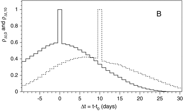
Figure 4. For the mlcs2k2 model, correlation coefficient ρΔt,0 between B-band epoch at peak brightness (t0) and time Δt = t − t0, where ρΔt,0 ≡ cov(Δt, 0)/σΔtσ0, as a function of Δt, and correlation coefficient  between epoch at 10 days past peak (t10) and time t − t10. The spikes at 0 and 10 days correspond to the requirements ρ0,0 = 1 and ρ10,10 = 1.
Download figure:
Standard image High-resolution imageSome example fits for SDSS-II SN light curves using the modified version of mlcs2k2 are shown in Figure 1. Figure 5 shows the average fractional residuals between the mlcs2k2 model light curves and the data for the SNe in each survey and for each rest-frame UBVR passband. The overall data-model agreement is good, except for some late-time epochs and U band. The U-band residuals are discussed later in more detail (Section 10.1.3). Figure 6 shows the fit parameters AV and Δ versus redshift for SNe in the different surveys. The impact of the prior requiring AV > 0 is immediately evident in the top-left panel. If we split each SN sample at its median redshift, the average AV for the lower-redshift SNe is larger than for the higher-redshift SNe; this AV difference is 0.1 mag for the Nearby sample, and ∼0.05 mag for the other SN samples. The prior discussed above accounts for this redshift-dependent shift. The right panel in Figure 6 shows the fitted AV versus redshift using a flat prior, P(AV) = P(Δ) = 1 in Equation (5). Although there are many SNe with AV < 0, in Section 7.3 we show that an underlying extinction distribution with AV > 0, combined with measurement uncertainties, is consistent with the "negative-AV" distribution obtained from fitting with a flat prior. Since Δ is well constrained by the light-curve fits, the Δ distribution with a flat prior is very similar to that using the nominal prior.

Figure 5. Data-model fractional residuals as a function of rest-frame epoch in five-day bins for mlcs2k2 light-curve fits. The rest-frame passband and SN sample are indicated on each plot. Measurements with S/N <6 are excluded, and error bars indicate the rms spread. For SNLS, the residuals are shown only for SNe with z < 0.5 as explained later in Section 10.2.4. Fdata (Fmodel) is the SN flux from the data (best-fit mlcs2k2 model). Vertical dashed lines indicate epoch of peak brightness (Trest = 0); horizontal dashed lines indicate Fdata = Fmodel.
Download figure:
Standard image High-resolution image
Figure 6. Left panels: mlcs2k2 fitted dust extinction values AV vs. redshift, for the different SN Ia samples indicated on the plot. Right panels: fitted Δ vs. redshift. Upper panels are from fit with nominal prior; lower panels are from fit with flat prior.
Download figure:
Standard image High-resolution imageWe have checked the results of the modified mlcs2k2 fitter with the distance estimates derived by WV07 for the ESSENCE and Nearby SN samples. For this comparison, we use the WV07 extinction prior and efficiency, as described in their Equations (2) and (3). The WV07 efficiency function accounts for missing SNe at high redshift and for the bias arising from using only measurements with S/N >5; for comparison, we therefore use the same S/N cut. The modified fitter is run in a mode that replicates the original mlcs2k2 fitter, with two exceptions: first, as noted above, we fit in flux instead of magnitude. Second, the K-corrections use the average spectral template of Hsiao et al. (2007), while WV07 used a library of spectra and interpolated K-corrections to the desired epoch. To compare our "Nearby+ESSENCE" analysis with WV07, we fit light curves for the 45 Nearby SNe Ia (0.015 < z < 0.1) and 57 ESSENCE SNe Ia analyzed by WV07. The rms scatter between our fitted distance moduli (μ) and those from WV07 is 0.03 mag and 0.05 mag for the Nearby and ESSENCE samples, respectively. Our marginalized value for the dark energy equation of state parameter w, using the SDSS BAO prior (see Section 8), agrees to within 0.01 with the result of WV07.
We stress that this comparison with WV07 is a consistency check of our version of mlcs2k2 relative to previous versions. When we analyze the present SN samples with mlcs2k2 (Section 10), our different prior and mlcs2k2 model parameter values result in cosmological parameter estimates that differ significantly from those of WV07, as discussed in Section 10.1.4.
5.2. salt-ii Fitting Method
The salt-ii light-curve fitting method (Guy et al. 2007) has been developed by the SNLS collaboration. The salt-ii model employs a two-dimensional surface in time and wavelength that describes the temporal evolution of the rest-frame spectral energy distribution (SED) for SNe Ia. The temporal resolution of the model is 1 day, and the wavelength resolution is 10 Å, allowing accurate synthesis of model fluxes to compare with photometric data. The model is created from a combination of photometric light curves and hundreds of SN Ia spectra. When there are measurement gaps in the spectral surface, the unmeasured regions of the SED are determined from interpolations of the measured regions. The photometric data are mostly from the Nearby sample (JRK07) but also includes higher-redshift data (z > 0.1) to better constrain the rest-frame ultraviolet behavior of the model. For a complete list of SN light curves and spectra used for training, see Table 2 in Guy et al. (2007).
In salt-ii, the rest-frame flux at wavelength λ and time t (t = 0 at B-band maximum) is modeled by
M0(t, λ), M1(t, λ), and CL(λ) are determined from the training process described in Guy et al. (2007). The M0 surface represents the average spectral sequence, and is very similar to the sequence of average spectral templates (Hsiao et al. 2007) that we use for the mlcs2k2 K-corrections. M1 is the first moment of variability about this average, accounting for the well-known correlation of both peak brightness and color with light-curve shape, and x1 is the stretch parameter, the analog of the mlcs2k2 Δ parameter. CL(λ) is the mean color correction term, and c is a measure of SN Ia color. Although the color variation is not explicitly attributed to dust extinction, in the optical region CL(λ) is reasonably well approximated by the CCM89 extinction law with RV ∼ 2. In the UV region, CL(λ) exceeds the CCM89 extinction by about 0.07 mag.
The spectral-time surfaces are defined for rest-frame times −20 < Trest < +50 days relative to the time of maximum brightness, and for rest-frame wavelengths that span 2000 to 9200 Å. We use the salt-ii spectral surfaces obtained from retraining the model using Bessell-filter shifts based on HST standards, as discussed in Appendix B (Table 21), but otherwise using the same technique and data as described in Guy et al. (2007). The UBVRI magnitudes for the primary reference Vega are taken from Fukugita et al. (1996): these are 0.02, 0.03, 0.03, 0.03, 0.024, respectively, and are slightly different from those used to crosscheck the mlcs2k2 method. Although the wavelength coverage of the spectral surface is rather broad, the salt-ii model includes only those observer-frame passbands for which  Å, where
  is the mean wavelength of the filter and z is the SN Ia redshift.
To compare with photometric SN data, the observer-frame flux in passband f is calculated as
where Tf(λ) defines the transmission curve of observer-frame passband f. For the SDSS-II, ESSENCE, SNLS, and HST samples, Tf(λ) is provided by each survey. For the Nearby sample, Tf(λ) is given by the Bessell (1990) UBVRI filter response curves, with wavelength shifts as described in Appendix B and listed in Table 21.
The model uncertainty accounts for the covariance between M0(t, λ) and M1(t, λ) at the same epoch and wavelength. Although spectral covariances between different epochs and wavelengths are not considered, the model does account for covariances between integrated fluxes at different epochs within the same filter. Each SN Ia light curve is fitted separately using Equations (6) and (7) to determine the parameters x0, x1, and c. However, the salt-ii light-curve fit does not yield an independent distance-modulus estimate for each SN. As discussed in Section 8.2, the distance moduli are determined as part of a global fit to an ensemble of SN light curves in which cosmological parameters and global SN properties are also determined. The salt-ii fits do not include informative priors on the fit parameters or the effects of selection efficiencies. We correct the salt-ii results for selection biases using a Monte Carlo simulation (see Sections 6 and 9.2).
In most cases, the salt-ii light-curve fits are qualitatively very similar to the mlcs2k2 fits on a per-object basis. The average rest-frame light-curve residuals for the salt-ii fits are shown in Figure 7 for each survey for filters UBVR; note that the U-band residuals for the Nearby SNe show some discrepancy, as will be discussed later. Figure 8 shows the fitted values for the color parameter c and stretch parameter x1 versus redshift for SNe in the different surveys.
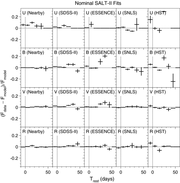
Figure 7. Data-model fractional residuals as a function of rest-frame epoch in five-day bins, for salt-ii light-curve fits. The rest-frame passband and SN sample are indicated on each plot. Measurements with S/N <6 are excluded. Note the discrepancy for the U-band residuals in the Nearby sample. For SNLS, the residuals are shown only for SN with z < 0.5 as explained later in Section 10.2.4. Fdata (Fmodel) is the SN flux from the data (best-fit salt-ii model). Vertical dashed lines indicate epoch of peak brightness (Trest = 0); horizontal dashed lines indicate Fdata = Fmodel.
Download figure:
Standard image High-resolution image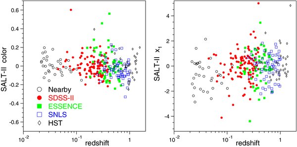
Figure 8. Left panel: salt-ii fitted color values (c) vs. redshift, for the SN Ia samples indicated on the plot. Right panel: fitted stretch parameter values, x1, vs. redshift.
Download figure:
Standard image High-resolution imageAs a crosscheck on our use of the public salt-ii code, we have compared our fits of the 71 SNe Ia from Astier et al. (2006) to fits done by the developer (J. Guy 2008, private communication) and find good agreement. The mean difference in the color (c) is 0.003 ± 0.003, with an rms dispersion of 0.02, and the mean difference in the shape-luminosity parameter (x1) is −0.014 ± 0.021, with an rms dispersion of 0.18. The slight differences are attributable to the use of different versions of the code and of the error (dispersion) map.
5.3. Comparison of mlcs2k2 and salt-ii Fitters
We end this section by briefly comparing and contrasting the salt-ii and mlcs2k2 methods. The mlcs2k2 rest-frame model for the intrinsic SN brightness is defined in discrete UBVRI passbands corresponding to the Landolt system. For each SN light curve, a composite SN spectrum is warped based on the model fit to the observed SN colors at each epoch, and the warped spectrum is used to perform the K-corrections needed to transform the rest-frame model to the observer-frame fluxes. The salt-ii model uses a composite SN spectrum that depends on both the epoch and intrinsic luminosity as well as an epoch-independent color term. This spectrum is used to model the rest-frame fluxes. Both the salt-ii and mlcs2k2 models are trained using Nearby SN Ia data, but salt-ii training also includes higher-redshift data that reduces the dependence on the Nearby SN sample and provides better constraints on the rest-frame ultraviolet regions of the spectrum.
The salt-ii parameters x1 and c are analogous to the mlcs2k2 parameters Δ and AV. The parameters x1 and Δ are essentially equivalent in describing the correlation between SN light-curve shape and brightness, but c and AV have different meanings. mlcs2k2 assumes that all intrinsic SN color variations are captured in the model by the light-curve shape-luminosity correlation and that any additional observed color variation is due to reddening by host-galaxy dust. The color term (c) in salt-ii describes the excess color (red or blue) of an SN relative to that of a fiducial SN with fixed stretch parameter x1. The excess color could be from host-galaxy extinction, from variations in SN color that are independent of x1, or from other effects, and salt-ii does not attempt to separate these effects. salt-ii uses c to reduce the scatter in the Hubble diagram in a manner analogous to the use of x1. The global salt-ii parameter β, defined below in Section 8.2, is the analog of the global mlcs2k2 dust parameter RB = RV + 1; one expects β ≃ RB if excess color variation is purely due to host-galaxy extinction. The salt-ii β parameter is determined from the global fit to the Hubble diagram for the entire SN Ia sample under analysis; we determine the mlcs2k2 RV parameter by modeling the observed colors of a specific subset of the SN data (Section 7.2).
Concerning correlations among model parameters, mlcs2k2 and salt-ii treat different aspects. The mlcs2k2 model includes covariances between different epochs and passbands, but we have excluded the off-diagonal covariances as explained in Section 5.1. The salt-ii model includes covariances between integrated fluxes at different epochs within the same passband, but covariances between passbands are not considered. salt-ii also includes the covariance between the spectral surfaces M0(t, λ) and M1(t, λ) at each epoch and wavelength bin (Equation (6)), but it does not include covariances between different epochs and passbands.
Within the mlcs2k2 framework, each light-curve fit yields an estimated distance modulus along with its estimated error, independent of cosmological assumptions. By contrast, in salt-ii the distance-modulus estimate for a given SN is based on a global fit to the ensemble of SNe within a parameterized cosmological model (see Section 8.2). A result of this global minimization in salt-ii is that a distance-modulus bias in a particular redshift range, such as could arise from including a poorly calibrated filter, will induce a bias over the entire redshift range of the sample. For the determination of cosmological parameters, this tends to reduce the sensitivity to systematic problems and hence can lead to smaller systematic uncertainties. However, this reduced sensitivity can also make biases more difficult to identify. An explicit example of this is described in Section 10.2.4.
Fitting with mlcs2k2 usually incorporates a Bayesian prior (Equations (3)–(5)) that reduces the scatter in the Hubble diagram by incorporating information about the underlying AV distribution and the survey efficiencies. The prior and the resulting Hubble scatter do not depend on cosmological parameters. Because of the assumption that excess color variation is due to extinction by dust, the prior excludes values of AV < 0. In mlcs2k2, SNe with very blue apparent colors (bluer than the template) are assigned AV ≃ 0, and the data-model color discrepancy is attributed to fluctuations. In salt-ii, apparently blue SNe are assigned negative colors (c < 0) that result in larger luminosities and distance moduli compared to mlcs2k2.
Within the salt-ii framework, scatter in the Hubble diagram is explicitly minimized by simultaneously adjusting global SN parameters along with the cosmological parameters; this minimization is described in Section 8.2. In contrast to mlcs2k2, the salt-ii Hubble scatter depends on the cosmological parameters, and there is no mechanism to account for the survey efficiency directly in the fits. To correct for biases related to the survey efficiencies (Section 8.2), we use the Monte Carlo simulations described in Section 6.
The mlcs2k2 and salt-ii light-curve fit residuals can be visually compared in Figures 5 and 7; the data and models are consistent for rest-frame passbands BVR, but there are discrepancies for U band in both cases. We address this issue in more detail in Sections 10.1.3 and 10.2.4, and we compare the mlcs2k2 and salt-ii results explicitly in Section 11.
6. MONTE CARLO SIMULATION: DETERMINING THE SELECTION EFFICIENCY
All surveys suffer from incompleteness and selection effects of various kinds. SNe that are intrinsically subluminous or highly extinguished by dust have less chance of being included in a flux-limited sample than more typical SNe. In addition, with limited spectroscopic resources, higher priority may be given to SN candidates with the best chances of yielding reliable identifications, e.g., by focusing on events that appear well separated from the host-galaxy or for which the host has either low surface brightness or early-type colors and morphology that suggest low dust content. These selection effects become more pronounced at the high-redshift end of a survey, where only the brightest, unextinguished SNe will satisfy selection cuts. If SN Ia brightness were a perfectly standardizable distance indicator, such selection effects would not be an issue for cosmological analysis. However, intrinsic variations in SN brightness, photometric errors, and uncertainties in estimating host-galaxy dust extinction lead to significant uncertainties and possible biases in distance estimates, particularly for SNe observed with low signal to noise. In order to extract unbiased cosmological parameter estimates, biases must either be reduced to an acceptably small level by the analysis procedure or else a correction scheme must be adopted.
We have developed detailed Monte Carlo simulations of the different SN surveys in order to determine the survey selection (or efficiency) functions and their impacts on SN distance estimates for both mlcs2k2 and salt-ii. The simulations also enable us to verify the estimates of systematic errors due to uncertainties in the light-curve model parameters. The simulated efficiency is a major component in the mlcs2k2 fit prior discussed above in Section 5.1. Determining the host-galaxy extinction dependence of the efficiency is critical for the mlcs2k2 method, because the extinction is often poorly determined from the data. For the salt-ii method, the simulation and efficiency play no direct role in the fitting, but they enable us to estimate and correct for biases in the cosmological parameters as described in Section 8.2.
Ideally, survey simulations would be based on artificial SNe Ia embedded into survey images, as was done during the SDSS-II SN survey to monitor the efficiency of the search pipelines (see Section 2). We do not have access to the images for the other surveys, and full image-level simulations would require a large amount of computing to perform the many variations that are needed for the analysis. We have instead developed a fast light-curve simulation40 that is based upon actual survey conditions and that therefore accounts for non-photometric conditions and varying time intervals between observations due to bad weather. At each survey epoch and sky location, the simulation uses the measured PSF, zero point, CCD gain, and sky background to determine the noise and to convert the simulated model magnitudes into CCD counts. The simulation also incorporates a model for host-galaxy light and dust extinction. We have obtained the necessary observational information for the SDSS-II, ESSENCE, SNLS, and HST surveys to carry out these detailed simulations. The Nearby SN Ia sample is a heterogeneous sample collected over many years by different observers and telescopes, and we do not have the information needed to make detailed simulations of this sample.
Here we describe the simulation within the context of the mlcs2k2 light-curve model and comment on the differences needed to simulate light curves in the salt-ii model. We select a random SN redshift from a power-law distribution, dN/dz ∼ (1 + z)β, with β = 1.5 ± 0.6, as determined by our recent analysis of the SN Ia rate (Dilday et al. 2008). An SN Ia luminosity parameter Δ and host-galaxy extinction AV are selected from underlying distributions that we have inferred from our data (Section 7.3). The mlcs2k2 model is used to convert Δ into rest-frame UBVRI magnitudes. These generated SN Ia magnitudes are increased according to the selected AV and the CCM89 extinction law using RV = 2.18, as determined in Section 7.2. The reddened UBVRI magnitudes are K-corrected into observer-frame magnitudes. A random sky coordinate is selected from the survey area, and Milky Way extinction is applied based on the maps of Schlegel et al. (1998). A random date for peak brightness is selected from the survey time frame, and all observed epochs at the selected sky coordinate are identified from the actual survey observations. For each observation epoch, the measured survey zero point is used to convert the simulated magnitude into a simulated flux. For simulations based on the salt-ii model, the mlcs2k2 parameters Δ and AV are simply replaced by the corresponding salt-ii parameters (x1, c), drawn from empirical distributions.
The simulated noise for each epoch and filter includes Poisson fluctuations from the SN Ia (signal) flux, sky background, CCD read noise, and host-galaxy background. The signal noise is based on the number of CCD photoelectrons calculated from the simulated flux. The sky background is computed from the measured sky background per pixel, which is summed over an effective aperture based on the measured PSF at that survey epoch and sky coordinate. For SN redshifts  , noise from the host galaxy is simulated by associating the SN with a host from the SDSS galaxy photometric redshift catalog (Oyaizu et al. 2008), randomly selected such that zgal ∼ zSN. From the SDSS DR5 (Adelman-McCarthy et al. 2007) photoPrimary database (Stoughton et al. 2002), we use the fitted exponential surface brightness profile in the r band as a probability distribution from which the SN position within the galaxy is randomly selected, i.e., we assume that the SN Ia rate within a galaxy is proportional to the local r-band luminosity. The host-galaxy background is computed by integrating the exponential galaxy model within the same effective aperture that is used for the sky noise. The exponential profile is not appropriate for early-type galaxies, but this model is meant only as an estimate of the range of host-galaxy background light expected. The host-galaxy noise exceeds the sky noise for only ∼10% of the simulated SNe Ia with zSN < 0.4. For redshifts greater than 0.4, the lack of simulated host-galaxy noise is not significant, because the sky noise is dominant at these higher redshifts
There remain two important aspects of the simulation that are less well defined and therefore more difficult to model: (1) intrinsic variations in SN Ia properties, beyond the shape-luminosity correlation, that lead to (so far) irreducible scatter in the Hubble diagram; and (2) search-related inefficiencies beyond those due to photometric signal to noise and selection cuts, e.g., those associated with spectroscopic selection. Below, we describe our modeling of these features in the simulation.
6.1. Simulating Variations of Intrinsic SN Brightness
Using the mlcs2k2-based simulation described above, the resulting scatter in the Hubble diagram for SDSS-II SNe at z < 0.15 is only 0.06 mag, well below the observed scatter of ∼0.15 mag. To make the model more realistic, we introduce intrinsic fluctuations in the simulated luminosity. The models for intrinsic fluctuations described below are empirically determined to match the observed Hubble scatter and are not based on a physical model.
We have implemented two models of intrinsic SN variations. The default method we use for mlcs2k2, called "color smearing," introduces an independent fluctuation in each passband, and the fluctuation is the same for all epochs within each passband. A random number  from a unit-variance Gaussian distribution is chosen for each rest-frame passband f'. A magnitude fluctuation,
  , is added to the generated magnitude at all epochs, where
  is the magnitude uncertainty at peak brightness given by the mlcs2k2 model in passband f'. In this method, the intrinsic model colors are randomly varied by typically ∼0.1 mag. Since the simulated color variations are the same at all epochs, this model does not respect the Lira law (Phillips et al. 1999), the empirical observation that intrinsic SN Ia colors have smaller variations at epochs later than about two months after explosion; this deficiency has a negligible impact on our analysis because our requirements of good light-curve coverage make our simulated efficiencies insensitive to the magnitudes at such late epochs.
The second model of intrinsic variation, which we use for the salt-ii method, and as a crosscheck for the mlcs2k2 method, is called "coherent luminosity smearing:" a coherent random magnitude shift, typically ∼0.15 mag, is added to all epochs and passbands. In the coherent smearing method, the intrinsic model colors are not varied.
A caveat in our implementation of intrinsic luminosity variations is that the mlcs2k2 simulation and fitter use different models of intrinsic fluctuations and covariances. Although the mlcs2k2 model includes a full covariance matrix, we argued in Section 5.1 that these covariances do not accurately reflect intrinsic correlations. Since we use only the diagonal elements of the mlcs2k2 covariance matrix in the fitter, a literal translation for the simulation would be to implement a random intrinsic fluctuation of ∼0.1 mag independently for each epoch and passband. Since the observed smoothness of high-quality SN Ia light-curve data rules out such large intrinsic epoch-to-epoch fluctuations, we have chosen the above methods to simulate intrinsically smooth light curves. In future training of SN Ia light curves, it will be desirable to extract a model of intrinsic fluctuations and covariances that can be used consistently in both the light-curve fitter and the simulation.
6.2. Simulation of Survey Search Efficiency
The final step in the simulation is to model losses related to the SN search. In particular, we need to account for SNe Ia that would have passed the light-curve selection cuts of Section 4 had they been identified, but that were missed due to inefficiencies in the SN search.
Search-related losses come from the following sources: (1) the image-differencing pipeline can fail to detect objects with very low signal to noise as well as objects with nearby artifacts such as a diffraction spike; (2) humans tasked with evaluating objects detected in subtracted images may not correctly identify them as possible SN candidates; (3) software used in spectroscopic targeting to fit light curves and photometrically classify SN candidates identified by humans may not correctly classify all SNe Ia; and (4) due to limited resources for spectroscopic observations, not all photometrically identified SN Ia candidates will be targeted spectroscopically or result in a spectrum with sufficient signal to noise to confirm the SN type and determine its redshift.
We define the overall survey efficiency, or survey selection function, as survey = search × cuts, where the search efficiency is further decomposed as search = subtr × spec. Here, subtr describes the net search efficiency of the image-subtraction pipeline corresponding to step (1) above. The term spec describes the combination of steps (2), (3), and (4), which depends in part on human judgment for each SN, and cuts is the factor associated with the final selection cuts described in Section 4. These decompositions of efficiency components are convenient because, if sufficient information about the search is available, then cuts and subtr can be reliably simulated. By contrast, it is usually impossible to directly simulate spec because it involves complex decision making under varying circumstances by many people involved in spectroscopic observations. However, if the spectroscopic efficiency is nearly 100% below some redshift for a given survey, then we can model spec at higher redshifts by comparing observed distributions of SNe properties (including redshift) to simulated distributions expected for a spectroscopically complete survey. In summary, our philosophy is to make as detailed a model of the survey efficiency components as the data and survey information allow, and to use data-simulation comparisons to constrain the other components.
The different components of the efficiency are likely to be correlated, so that the overall efficiency is not really a simple product as defined above. As an extreme example, if both the search and selection cuts required only that the maximum S/N was greater than 5, then search = cuts, and the combined efficiency would be the same (not the product of the two). As discussed below for the SDSS-II survey, we can simulate the combined effect of the image-subtraction efficiency (subtr) and selection cuts (cuts). To simplify notation we write the combined efficiency as a product, subtr × cuts, but it should be understood that this product really refers to the combined efficiency taking into account all correlations. The spec term is treated differently in that it is defined as an independent efficiency function that multiplies the other efficiency terms.
For the SDSS-II, ESSENCE, SNLS, and HST samples, we have obtained detailed observing conditions, and the simulation accurately describes the effects of sample selection criteria, cuts. For the SDSS-II, we determine subtr using information from the fake SNe Ia that were inserted into the images during the survey (see below). For the non-SDSS samples, we do not have access to the pixel-level data, so we set subtr = 1 and absorb the image-subtraction pipeline efficiency into the spectroscopic efficiency, spec = search. For the Nearby sample, we do not even have the information needed to determine the impact of the selection cuts; we therefore absorb all sources of inefficiency into the spectroscopic efficiency, spec = survey.
As noted above, for the SDSS-II, fake SNe Ia are used to infer subtr as a function of S/N, as shown in Figure 7 of Dilday et al. (2008). These efficiency curves are used by the light-curve simulation to probabilistically determine which measurements in which passbands result in detections; a single-epoch detection in any two of the three (gri) passbands is considered to be an object. An object found at two or more epochs results in an SN candidate and is considered to be discovered by the image-subtraction pipeline. For the SDSS-II, the image-subtraction pipeline efficiency (subtr) is complete up to a redshift of z ∼ 0.2 and then drops gradually to about 60% at z ≃ 0.4.
For the HST simulation, we use the single-epoch search efficiency as a function of magnitude, as described in Strolger et al. (2005) and Strolger & Riess (2006). The search was done with the F850LP_ACS passband (mean wavelength: 9070 Å); it is fully efficient down to mag ∼23, and the efficiency drops to half at mag ∼26. Incorporating this single-epoch efficiency profile into our simulation and requiring any one detection to discover an SN, the simulated efficiency for finding SNe Ia is 100% up to z ∼ 1, and drops to about 65% at z = 1.6.
6.2.1. Modeling Spectroscopic Efficiency
Although selection effects associated with the photometry can be simulated based on available information, modeling the spectroscopic efficiency for each survey is more of a challenge. The SN redshift distributions N(z) for the non-HST data and simulations are shown in Figure 9. With the exception of the Nearby SN sample, the simulations include losses from selection requirements (Section 4); for SDSS-II, losses from the image-subtraction pipeline are also included. For the Nearby sample, the simulation is based on SDSS-II observing conditions and is chosen to be 100% efficient, since we do not have the information to model the effects of photometric selection requirements in that case; the simulated redshift distribution in narrow bins of redshift therefore scales as N(z) ∼ z2 (ignoring evolution of the SN Ia rate at low redshift).
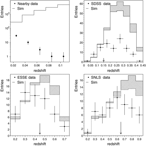
Figure 9. Comparison of redshift distributions for data (dots) and simulations (histograms) for the Nearby (JRK07), SDSS-II (2005 data only), ESSENCE (Wood-Vasey et al. 2007), and SNLS (Astier et al. 2006) samples. The Nearby sample is shown on a logarithmic scale, while the other vertical scales are linear. The simulations include losses from selection requirements (Section 4), and, for the SDSS-II, losses from the image-subtraction pipeline. The shaded regions show uncertainties in the simulated distributions due to uncertainty in the SN Ia rate vs. redshift (β = 1.5 ± 0.6 for dN/dz ∼ (1 + z)β). Except for the Nearby sample, the simulated distributions are scaled such that the integrated number of simulated SNe left of the cutoff redshifts (indicated by vertical arrows) match the data. Vertical error bars show the statistical uncertainty; horizontal bars show the bin size.
Download figure:
Standard image High-resolution imageBelow some cutoff redshift, zcut, the spectroscopic efficiency is assumed to be ∼100%; for z > zcut the data-simulation discrepancy in N(z) is taken to be due to spectroscopic inefficiency. For the SDSS-II and SNLS samples, the cutoff redshifts are estimated to be 0.15 and 0.65, respectively, based on the levels of completeness given in their SN Ia rate measurements (Dilday et al. 2008; Neill et al. 2006). For the ESSENCE sample, we estimate zcut ∼ 0.45 based on visual inspection of the redshift histogram in Figure 9. For the Nearby (z < 0.1) sample, there is no redshift below which the spectroscopic completeness is assumed to be 100% (see discussion below). All four of these samples show significant spectroscopic inefficiency at the upper ends of their redshift ranges.
The data-simulation redshift comparison for the HST sample is shown in Figure 10. Although the uncertainty in the SN Ia rate at these high redshifts is large, there is no evidence for significant spectroscopic inefficiency: the data-simulation redshift comparison is consistent with the claim that there are no significant losses for z < 1.4 (Riess et al. 2007). We therefore assume that spec = 1 for the HST survey, and this sample is not included in the efficiency discussion below.
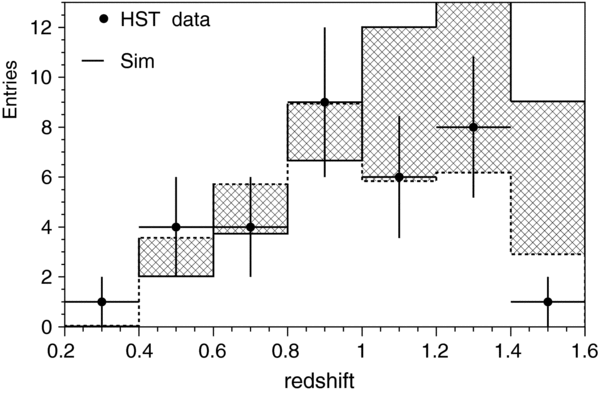
Figure 10. Redshift distribution for HST sample (Riess et al. 2007); data are shown by dots and the simulation by a histogram. The shaded region shows the uncertainty from the redshift dependence of the SN Ia rate (see the caption to Figure 9), but with the rate uncertainty doubled for z > 1.
Download figure:
Standard image High-resolution imageThe spectroscopic efficiency as a function of redshift is defined to be spec ≡ survey/(subtr × cuts), which corresponds to the ratios of the data and simulation histograms in Figure 9. For each sample, this efficiency can be fitted by an exponential function,
where ζ0 and ζ1 are determined from the fit. The discontinuity at zcut is motivated by the SDSS-II survey, for which our spectroscopic observation strategy targeted z < 0.15 candidates with very high priority. We have no evidence that the other surveys should have discontinuities in their redshift distributions, but the model above provides a reasonably accurate representation for the redshift distributions of the ESSENCE and SNLS samples as well. This functional form is adopted for computational convenience in generating large Monte Carlo samples.
Although the redshift dependence of the spectroscopic efficiency has now been estimated, we know that spec(z) depends in reality on a variety of factors, not simply redshift, and we must model its dependence on those factors in order to properly model the selection function and associated biases. As noted above, since spectroscopic targeting is a complex process, the underlying mechanism determining spec is not easily characterized. The simplest possibility would be that spec depends purely on redshift: in this case, zspec ≡ spec(z) would be given by Equation (8), and there would be no impact of spectroscopic efficiency on the survey bias, since redshift is precisely measured for each SN in the samples we consider. However, this model is not a priori likely: it is more probable that spec depends explicitly on both redshift and apparent SN Ia brightness, the well-known Malmquist bias.
To consider this alternative, we define a "magnitude dimming" parameter  as the difference between the simulated rest-frame magnitude and the magnitude of the brightest possible SN Ia at peak light in rest-frame V band (for mlcs2k2) or in rest-frame B band (for salt-ii). For the mlcs2k2 and salt-ii models,
  is given by

For mlcs2k2, AV is the host-galaxy extinction in the V band, p0,V and q0,V are model parameters at the epoch of peak brightness in the V band (see Equation (1)), and Δref = −0.3 corresponds to nearly the most intrinsically luminous SN Ia in the training sample. For the SDSS-II, ESSENCE, and SNLS samples, Θ = 1; for the Nearby sample, we set Θ = 0, because the Δ distribution for the Nearby sample appears unbiased relative to that of the underlying SN Ia population (see Section 7.3) while its AV distribution is clearly biased. For salt-ii, x1 and c describe the light-curve shape and color for each SN Ia (see Section 5.2),  and cref = −0.26 correspond to the brightest SN Ia, and α, β are global SN Ia parameters determined in the cosmology fit (see Section 8.2).
Using the magnitude dimming parameter, we model the spectroscopic inefficiency due to apparent magnitude as

where m(z) is an exponential slope function determined by numerically solving
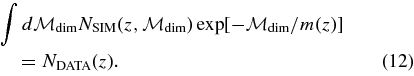
Here,  is the number of simulated events in a two-dimensional bin of redshift and simulated
  , and NDATA(z) is the number of data events in the redshift bin. In practice, m(z) is evaluated in discrete redshift bins for z > zcut and fit to an exponential function of redshift,

where m0, m1, and m2 are determined in the fit, and m(z) = ∞ for z < zcut. Since  is defined for V band in the mlcs2k2 model and for B band in the salt-ii model, the associated m0, m1 parameters are different. The parameter m2 is non-zero only for the Nearby sample. Qualitatively, Equation (11) says that SNe that are intrinsically faint (large positive Δ) or extinguished (large AV) will be under-represented at the high-redshift end of a sample.
In principle, we now have two models for the spectroscopic efficiency: one, denoted by zspec, and explicitly given in Equation (8), depends solely on redshift; the other depends explicitly on apparent brightness and implicitly on redshift and is also constrained to match Equation (8). While the latter model corresponds to expectations for Malmquist bias, the "redshift-only" model zspec may be better suited to modeling spectroscopic selection that assigns lower priority to SN candidates near the cores of host galaxies, since SN-host angular separation tends to decrease with redshift. Since both models satisfy Equation (8), these two efficiency models can be linearly combined into a more general model:

To break this model degeneracy and determine the coefficient  , we compare the mean fitted extinction
  versus redshift for the data and the simulation after applying all efficiency factors, and we minimize the χ2 for the data-simulation difference. For the SDSS-II,
  , indicating that most of the search inefficiency is related to SN Ia apparent brightness. For the ESSENCE survey,
  , indicating that most of the search inefficiency is simply a function of redshift. For the SNLS sample, the best-fit
  ; however, since the data-simulation χ2 for
  is only 0.3 larger than the minimum χ2 at
  , there is essentially no information on
  . The large uncertainty on
  is in part due to the relatively small spectroscopic inefficiency for the SNLS. For the Nearby sample, there is no redshift range for which the sample is 100% efficient, and we therefore need an additional constraint to determine the efficiency parameterization. Noting that the mean fitted extinction drops rapidly with redshift for the Nearby sample (see Figure 11), we assume that
  . Figure 11 shows that the simulated efficiency works well in reproducing the strong extinction gradient in the Nearby sample.
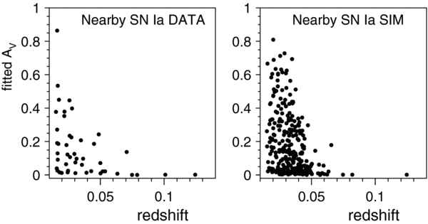
Figure 11. Left panel: mlcs2k2 fitted extinction AV vs. redshift for the Nearby SN Ia sample (JRK07). Right panel: fitted AV distribution for the simulation using the parameterized efficiency function of Equations (11) and (14) with  . Light-curve fits were made using the mlcs2k2 prior of Equation (5) and the exponential AV distribution of Section 7.2.
Download figure:
Standard image High-resolution imageAs an illustration, the inferred efficiencies for the SDSS-II SN sample are shown in Figure 12 as a function of AV, for different values of the redshift and shape-luminosity parameter Δ. The high quality of the simulation for the SDSS-II, ESSENCE, SNLS, and HST samples is illustrated in Figures 13 and 14, where we compare the observed redshift and flux distributions to simulations that include the efficiency functions derived above. The redshift comparisons have excellent χ2/dof as a result of how the spectroscopic efficiency is determined. For the flux comparisons, the χ2/dof vary from 1 to a few; the larger χ2 values are due to a few notable discrepancies in some of the flux bins.
Figure 12. Estimated efficiency vs. extinction for the SDSS-II SN sample. Each panel corresponds to a different combination of redshift (z = 0.1, 0.3) and intrinsic SN Ia brightness (Δ = −0.3, + 0.5→ bright, faint). The curves correspond to different stages of the efficiency: after the image-subtraction pipeline, subtr (dotted); after spectroscopic confirmation, search = subtr × spec (dashed); and after selection cuts, survey = search × cuts (solid). For z = 0.1, the spectroscopic efficiency is 100%, so the search (dashed) and image-subtraction (dotted) curves are the same. In all cases, cuts ∼ 0.8 at low extinction; this loss is mainly due to the requirement of good light-curve coverage, i.e., SNe that peak very early or very late in the observing season do not have adequately sampled light curves to satisfy the selection criteria.
Download figure:
Standard image High-resolution image
Figure 13. Comparison of redshift distributions for data (dots) and simulations (histograms), for the SDSS-II, ESSENCE, and SNLS samples after applying the selection requirements in Section 4. The simulations include all known effects, including the spectroscopic inefficiency. Each simulated distribution is scaled such that the total number of SNe matches the data. The SDSS data-simulation discrepancy for z > 0.4 is an artifact of our simple modeling of spec (Equation (13)).
Download figure:
Standard image High-resolution image
Figure 14. Comparison of flux distributions for data (dots) and simulations (histograms) for SDSS-II, ESSENCE, SNLS, and HST. The observer-frame passband is indicated on each plot (HST filter symbols are 0 = NIC-F110W, 1 = NIC-F160W, 2 = ACS-F606W, 4 = ACS-F775W, 6 = ACS-F850LP). Each simulated distribution is scaled to have the same total number of entries as the data; bins with zero entries are not plotted. The calibrated flux is 10−0.4 mag+11. As in Figure 13, the simulations include all the survey inefficiencies.
Download figure:
Standard image High-resolution imageWe have also compared the distributions of the number of epochs, earliest and latest epochs, noise, and peak colors, and find good data-simulation agreement in these distributions as well.
7. ESTIMATION OF HOST-GALAXY DUST PROPERTIES
The Monte Carlo simulations used in the previous section to model survey selection functions rely on knowledge of host-galaxy dust properties, in particular on the underlying distribution of extinction, P(AV), and on the mean reddening law parameter, RV. Moreover, mlcs2k2 distance estimates rely directly on our knowledge of these two quantities, which are assumed to be independent of redshift. In this section, we describe how we determine these dust properties from the SDSS-II SN sample. These global dust properties are used in the mlcs2k2 fitting prior for all SN samples.
7.1. SDSS-II "Dust" Sample
The results of Section 6.2.1 indicate that current SN samples suffer from significant spectroscopic selection effects (see Figure 9). Since spectroscopic selection is likely to be biased against highly extinguished SNe, use of purely spectroscopic SN samples may lead to biased estimates of the distribution of host-galaxy dust properties and thereby to potentially biased distance estimates when a dust-distribution prior is applied. To address this issue, we use a nearly complete set of SDSS-II SNe Ia to measure dust properties. For SDSS-II events with SN Ia like light curves that were not spectroscopically confirmed as SNe Ia, we have embarked upon a program to obtain host-galaxy spectra and measure spectroscopic redshifts; we call these photometric SN Ia candidates. Based on distributions of the mlcs2k2 fit parameters as well as visual inspection of the light-curve fits, we find that the requirement of a good SN Ia light-curve fit (see cut 5 in Section 4) to a well-sampled light curve is a good substitute in identifying SNe Ia when a confirming SN spectrum is lacking.
To identify photometric SN Ia candidates, we start with all 4100 candidate events that were detected by the on-mountain frame-subtraction pipeline on two or more epochs in the 2005 observing season (see Section 2). We process these candidate light curves through SMP (Section 3.2), fit them with the mlcs2k2 method, and prioritize them for host-galaxy spectroscopy based on the quality of the light curve and the fit. We have obtained host-galaxy redshifts for the majority of candidates for which the host-galaxy r-band magnitude satisfies r ≲ 20 and for a large subsample of fainter hosts as well. Adding this "host-z" photometric SN Ia sample to the spectroscopically confirmed and probable SN Ia sample, the combined sample appears to be nearly spectroscopically complete to z ≃ 0.3, when compared with the simulated sample. For z < 0.3, after the selection cuts of Section 4 are applied, the combined sample comprises 81 confirmed SNe Ia, 6 probable SNe Ia, and 73 host-z SNe Ia. We refer to these 160 SNe Ia as the SDSS-II dust sample. To illustrate the importance of including the host-z subset, we note that the average fitted extinction (AV) is about 0.2 for the spectroscopically confirmed sample and almost 0.4 for the host-z sample: ignoring the host-z subset would clearly lead to biased results for the distribution of host-galaxy dust properties. On the other hand, giving highest priority to bright host galaxies for the host-z follow-up program may preferentially select hosts of more extinguished SNe.
To illustrate our understanding of the efficiency, Figure 15 shows the redshift distribution for the dust sample, compared with the simulation that includes known losses from the image-subtraction pipeline and selection cuts but does not include losses related to spectroscopic observations. This comparison shows that the dust sample is indeed nearly complete for redshifts z < 0.3. We can obtain an independent estimate of the dust-sample completeness by counting the number of photometric SN Ia candidates that pass our selection cuts, that have a photometric redshift (based on the host galaxy or the SN light curve) less than zphot = 0.3, and that have not yet been targeted for host-galaxy spectroscopy. There are nearly 40 such events, indicating a completeness, after selection cuts, of about 80% for the dust sample at z < 0.3.

Figure 15. Redshift distribution for the SDSS-II dust sample (dots), which includes confirmed, probable, and host-z photometric SN Ia events, and for the simulation (histogram), which includes losses from the image-subtraction pipeline and selection cuts. Shaded region reflects simulated uncertainty in the SN Ia rate as explained in the caption to Figure 9. Vertical arrow indicates z < 0.3 requirement to select the dust sample used for the determination of host-galaxy dust properties.
Download figure:
Standard image High-resolution image7.2. Determination of Dust Reddening Parameter RV
Although RV varies along sight lines through the Milky Way and likely varies with local environment within galaxies, we follow standard practice in treating it as a global parameter, because most current SN data are not adequate to determine it on an object-by-object basis. After briefly reviewing previous determinations of RV, we describe the method we have developed to determine RV and its results.
Measurements of dust properties in the Milky Way have favored an average value of RV ∼ 3.1 (Fitzpatrick & Massa 2007) along sight lines with moderate to substantial extinction, and this has been used as a canonical value in the literature. However, studies of stellar colors in the direction of several thin cirrus clouds in the Milky Way indicate a value of RV ∼ 2 for those relatively low-extinction environments (Szomoru & Guhathakurta 1999). For galaxies that host SNe Ia, two methods have been commonly used to determine RV. The first infers an average or global RV value based on statistical averages of optical light-curve colors. This method has been applied to the Nearby SN sample (Phillips et al. 1999; Altavilla et al. 2004; Reindl et al. 2005; Riess et al. 1996; Nobili & Goobar 2008), resulting in RV values in the range of 2–3, somewhat lower than the Milky Way average value. The second method uses SNe Ia that have densely sampled, high signal-to-noise optical and NIR photometry, for which RV can be estimated for individual events: this method has resulted in RV ∼ 1–2 (Krisciunas et al. 2007, 2006; Elias-Rosa et al. 2006; Wang et al. 2008), significantly below the canonical Milky Way value. Calculations and simulations have shown that multiple scattering by circumstellar dust can lead to lower values for the reddening parameter inferred from SNe Ia, RV ∼ 1.5–2.5 (Wang 2005; Goobar 2008).
Within the framework of the mlcs2k2 light-curve model, we have used the SDSS-II dust sample and a variant of the average color method to make a new determination of RV. Previous measurements with this method were based on samples with large and unknown selection effects; our determination of RV is based upon an SN Ia sample with a well-understood selection efficiency. We assume that reddening is due to dust extinction with a wavelength dependence described by the CCM89 model and that the mlcs2k2 model parameters (M, p, q in Equation (1)) accurately describe the SN Ia brightness and colors. The measurement of RV is based upon comparing the average colors as a function of SN epoch of the SDSS-II data to those of the simulation. By using the nearly complete z < 0.3 dust sample, we minimize potential selection bias against extinguished SNe Ia; this sample also has a selection efficiency that is well described by the simulation.
For the dust sample, we compute three mean observed SN Ia colors, g − r, r − i, and g − i, in one-day bins in rest-frame epoch, as shown in Figure 16. Although the third color (g − i) is redundant in most cases, it provides information in the few cases in which the r-band measurement is not available. The rest-frame time is relative to the time of peak brightness in the B band as determined by the mlcs2k2 light-curve fit (see Section 5.1). While the light-curve fits include all observations regardless of signal to noise, the estimates of the mean observed colors include only those observations for which the S/N is greater than 4. Since the g, r, i measurements are taken simultaneously in SDSS-II, the colors are determined directly from the data without the need to interpolate in time.
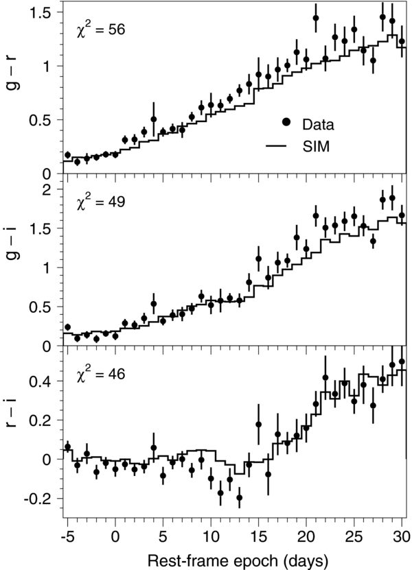
Figure 16. Mean SN Ia colors 〈g − r〉, 〈g − i〉, and 〈r − i〉 vs. rest-frame epoch, for the SDSS-II SN dust sample. Data are shown by the filled circles; the histogram overlay shows the simulation using the best-fit values of RV and  . The data-simulation χ2 (for 36 degrees of freedom) is indicated on each panel.
Download figure:
Standard image High-resolution imageWe compare these color-versus-epoch measurements with those of a grid of simulated samples, where each sample is generated with a different value of RV and  , and where
  describes the generated AV distribution, with
  . The RV and
  grid sizes are 0.2 and 0.05, respectively. The simulated and data samples are subject to the same selection cuts and fit with mlcs2k2 in the same way. We determine the best-fit values of RV and
  by minimizing the following χ2 statistic between the data and the grid of simulations,
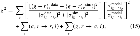
where the epoch-index e runs over 1-day bins with −5 < Tirest < 30 days, the data averages 〈〉datae are taken over all dust-sample SNe and epochs e surviving the cuts above, and the measured colors in the simulated samples depend upon the input values of RV and  . Each color uncertainty, e.g.,
  , is estimated as
  , where Ne is the number of color measurements (summed over all SNe) at epoch e. The second term in brackets is a weighting to account for the mlcs2k2 model uncertainty;
  is the minimum model uncertainty at the epoch of peak brightness, and
  is the model uncertainty at epoch e. The model-uncertainty ratio is therefore unity at Trest = 0 and decreases as the model uncertainty increases for epochs away from peak brightness, so that epochs with large errors are downweighted. We have tested this method with 100 simulated mock data samples as described in Section 6; the input values of RV and
  are recovered, and the statistical uncertainties, although they are smaller than the grid sizes, match the spread in recovered values.
Using the SDSS-II data and simulations, we find


and a correlation coefficient of 0.17. The relatively small correlation coefficient confirms that the method is independently sensitive to RV and  . Figure 16 compares the average observed colors with those of the simulation using the best-fit values in Equation (16). The χ2 values are somewhat larger than expected, particularly for g − r. There is also a notable data-simulation discrepancy for epochs past about 10 days for the g − r and g − i colors, although these late-time epochs carry less weight in the χ2 due to the increasing model errors.
To estimate the systematic uncertainties in this measurement, we have varied aspects of the procedure and determined their effects on the recovered RV and  . In particular, we lowered the redshift cutoff for the dust sample to z < 0.25 (nominal is 0.3), varied the simulated redshift distribution of the underlying SN Ia population, dN/dz = α(1 + z)β, within the correlated 1σ errors on α and β from Dilday et al. (2008), varied the minimum epoch from −10 to 0 days (nominal is −5 days), varied the maximum epoch from +25 to +35 days (nominal is +30 days), varied the minimum signal to noise between 2 and 8 (nominal is 4), excluded each of the three colors g − r, g − i, and r − i individually from the χ2 minimization, and ignored the mlcs2k2 model-uncertainty terms in the χ2 statistic. We also ran the simulation without intrinsic color fluctuations (see Section 6.1). The changes due to each of these variations to the nominal results for RV and
  were added in quadrature to obtain an estimate of the total systematic uncertainty. Table 3 summarizes the contributions to the systematic uncertainties. The largest source of uncertainty comes from reducing the redshift range from 0.3 to 0.25, which changes RV by 0.36 ± 0.17, and the error reflects the uncorrelated uncertainty. Although this RV shift is marginally consistent with a random fluctuation, we have included the shift as a systematic error.
Table 3. Summary of Uncertainties for the Determination of RV and 
| Source | σ(RV) |  |
|---|---|---|
| Statistical | 0.14 | 0.026 |
| Redshift range 0.25 − 0.3 | 0.36 | 0.031 |
| Assumed dN/dz: β = 0.9 − 2.1 | 0.11 | 0.004 |
| Epoch range | 0.25 | 0.045 |
| S/N >2, 8 | 0.11 | 0.011 |
| Exclude one color | 0.08 | 0.030 |
| Ignore mlcs2k2 model uncertainty | 0.05 | 0.018 |
| Remove color-smearing model | 0.14 | 0.017 |
| Total systematic | 0.48 | 0.068 |
| Total uncertainty | 0.50 | 0.072 |
Download table as: ASCIITypeset image
As a crosscheck of how the inferred RV depends on the assumed exponential form of the extinction distribution, P(AV), we have repeated the procedure using different distributions for AV in the simulation. In particular, we use a flat, truncated AV distribution, P(AV) = 1 for  , and P(AV) = 0 when
  ; this results in a negligible change in the inferred values of RV and
  . Thus, the inferred value of RV appears to be insensitive to the assumed AV distribution.
7.2.1. The salt-ii Approach to Measuring RV
The salt-ii analog of RV (called β, see Equation (29)) is determined by a very different method that involves minimizing the residual scatter in the Hubble diagram. For comparison, we have tried a similar procedure within the mlcs2k2 framework, selecting the global value of RV that minimizes the scatter in the Hubble diagram. For this test, we select spectroscopically confirmed SNe Ia from the SDSS-II sample that satisfy the light-curve criteria of Section 4 and that have redshifts z < 0.15; the resulting sample includes 24 SNe Ia. We concentrate on this low-redshift sample because it is nearly complete and because the measurement uncertainty on each distance-modulus estimate is well below the intrinsic scatter. The resulting Hubble scatter-minimized RV value is about 1.7, roughly 0.5 below our nominal result in Equation (16). This result holds whether we use the default prior (Equation (5)) or a flat prior in the light-curve fits. When we apply this procedure to the larger SDSS-II dust sample (Section 7.1) that extends to z = 0.3, the Hubble scatter-minimized RV value is slightly smaller. Hicken et al. (2009b) have applied the same approach to the Nearby CfA3 sample (Hicken et al. 2009a) and find that RV = 1.7 minimizes the Hubble scatter, consistent with our results for the SDSS-II samples.
To test this approach to extracting RV, we have implemented it on the simulated SDSS-II SN sample (Section 6). We generate a set of light curves with fixed RV and fit them with mlcs2k2 in the same way that the data are fitted. For the default color-smearing model of intrinsic SN luminosity variation (see Section 6.1), the Hubble scatter-minimized RV extracted from this process is biased low by 0.5 with respect to the input value. This bias is consistent with the difference we see between the scatter-minimized RV and the RV we infer from the mean colors of the SDSS-II dust sample. For the alternative "coherent luminosity smearing" model, however, which results in no intrinsic color variations, the scatter-minimized RV is unbiased.
While the result above is suggestive, an important caveat is that we have not evaluated the uncorrelated systematic uncertainty on the difference between our nominal RV extraction and the scatter-minimized RV. Our study suggests, however, that the salt-ii β parameter could be biased low if the color-smearing model is a reasonable description of intrinsic SN Ia luminosity variation.
7.3. Determination of the Underlying Distributions of AV and Δ
The mlcs2k2 simulation and the prior used in the mlcs2k2 fitting method require knowledge of the underlying distribution for the V-band extinction due to host-galaxy dust, P(AV). The distribution is also needed for the shape-luminosity parameter Δ, although the latter has less impact on the results, because Δ is better-determined by the light-curve data for each SN. We determine these distributions using the Bayesian unfolding method of D'Agostini (1995), which essentially uses underlying trial distributions in the simulation to make predictions for the observed distributions of fitted AV and Δ. To limit selection biases in this procedure, we use the SDSS-II dust sample of Section 7.1.
We fit the SDSS-II light curves with mlcs2k2 using a flat prior on AV, i.e., the fitted AV value is allowed to be negative. In the fit, the extinction as a function of wavelength is given by the CCM89 model with RV = 2.18, as derived in Section 7.2. The underlying distributions for AV and Δ are determined such that when they are input into the simulation, the fitted distributions from the simulated light curves match the distributions from the mlcs2k2 fits to the SDSS-II data. Technical descriptions of this procedure and of the assumed underlying distributions are given in Appendix D.
The results for the data and Monte Carlo simulation are shown in Figure 17. Although the generated AV distribution includes only non-negative values of AV, there is a tail of fitted negative values that is well described by the simulation and arises from photometric errors and intrinsic SN color variations. Our procedure determines the underlying AV distribution without assuming a functional form for P(AV), but it turns out that this distribution is well described by an exponential, P(AV) = exp(−AV/τV), with


The uncertainty in τV includes statistical and systematic uncertainties as described in Appendix D. The RV dependence is shown explicitly in Equation (18), along with the internal measurement error. Equation (19) shows the total uncertainty including the uncertainty on RV. The agreement between τV and  (from Section 7.2) is well within the expected dispersion based on simulated tests.

Figure 17. Fitted AV (left) and Δ (right) distributions, where the fits use the mlcs2k2 model with a flat AV prior. The measured SDSS-II dust sample distributions are shown by dots; the simulations are shown by histograms. The underlying (generated) AV distribution is shown by the dashed curve in the left panel.
Download figure:
Standard image High-resolution imageThe underlying AV distribution, including the uncertainties, is shown as the hatched region in Figure 18(a); we use this P(AV) as part of the mlcs2k2 prior in Equation (5). Our inferred AV distribution is marginally consistent with that of JRK07, who derived a prior of exponential form from the Nearby sample, with τJRKV = 0.46 (the dashed curve in Figure 18(a)). Our AV distribution is also somewhat consistent with the "galactic line-of-sight" (glos) prior, based on theoretical considerations (Hatano et al. 1998; Commins 2004; Riello & Patat 2005), that was used by WV07 for the ESSENCE analysis (the solid curve in Figure 18(a)).

Figure 18. (a) Underlying AV distributions, P(AV): dotted is from JRK07, solid is the glos distribution from WV07, and the hatched region shows the distribution used in this paper, derived from the SDSS-II SN dust sample; (b) underlying Δ distribution, P(Δ), used in the mlcs2k2 prior, also derived from the SDSS-II dust sample.
Download figure:
Standard image High-resolution imageThe underlying distribution of Δ is described by an asymmetric Gaussian with mean Δ0 = −0.24, and Gaussian widths of σ− = 0.24 for Δ < 0 and σ+ = 0.48 for Δ>0 (see Appendix D for uncertainties). As shown in the right panel of Figure 17, when input into the simulation this distribution leads to a distribution of fitted Δ that is in good agreement with the observed distribution of fitted Δ from the SDSS-II dust sample. The underlying Δ distribution, P(Δ), is shown in Figure 18(b). In addition to the asymmetric Gaussian, we have added a tail to the Δ distribution at positive Δ, allowing for underluminous SNe where the underlying distribution is poorly measured due to small-number statistics; when used in the mlcs2k2 prior of Equation (5), this tail ensures that the fitter is not heavily biased against underluminous SNe. Since Δ is well determined from the light-curve shape, the fitted value of Δ has little sensitivity to the functional form of P(Δ). To check the effect of the arbitrary tail in P(Δ), we have run the fits with amplitude of the tail region multiplied by half and by two; in both cases, the rms variation in fitted Δ is 0.01.
To check that the derived extinction distribution reflects that of the global SN population rather than that of a (possibly biased) SDSS-II sub-sample, we compare the fitted AV distributions for the data and for simulations generated with the underlying AV and Δ distributions derived above for each SN sample in Figure 19. Here, the fits are carried out with a flat AV prior, allowing AV < 0. The overall agreement is good for all samples. This test illustrates that the inferred negative extinction values (when an uninformative prior is used) are consistent with being artifacts of the combination of low signal to noise and intrinsic color fluctuations, since the simulation is generated with AV ⩾ 0. Note that the procedure used to determine the underlying AV distribution ensures that the data and simulation agree well for positive AV for the SDSS-II sample, but parameters have not been adjusted to match the distribution for the other samples, or for negative AV.
Figure 19. Comparisons of fitted AV distributions, using a flat prior, for data and simulations. Simulations were generated using the underlying AV distribution derived from the SDSS-II dust sample, with AV ⩾ 0. SN samples used in the cosmology analysis are indicated on each panel.
Download figure:
Standard image High-resolution image8. FITTING THE HUBBLE DIAGRAM FOR COSMOLOGICAL PARAMETERS
The estimation of cosmological parameters from SNe is based on measurements of the luminosity distance, dL, as a function of redshift. For a Friedmann–Robertson–Walker cosmological model, assuming the stress–energy comprises non-relativistic matter (M) and dark energy (DE) with constant equation of state parameter w = p/ρc2, the luminosity distance depends on four parameters: w, the matter density ΩM, the dark energy density ΩDE, and the Hubble parameter H0:
where the curvature density Ωk ≡ 1 − ΩM − ΩDE, and the function  for Ωk < 0,
  for Ωk > 0, and
  for a flat universe with Ωk = 0. The dimensionless expansion rate is given by
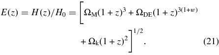
For this analysis, we assume that the dark energy equation of state parameter w does not evolve in time, mainly because current data do not yield precise constraints on the time derivative of w. For constraints on time-varying w, see Sollerman et al. (2009). Loosely, one can interpret the constraints we derive on constant w as constraints on the mean value of w(z) over the redshift interval 0 ≲ z ≲ 0.4. More precisely, one can interpret these constraints as providing information on one parameter in a two-parameter model that describes the evolution of w. That is, if the evolution of w is described by a linear two-parameter model, e.g., by w(z) = w0 + waz/(1 + z), then there is a pivot redshift zp at which the measurements of w0 and wa are uncorrelated and the error in wp ≡ w(zp) reaches a minimum. For the combined SN Ia data sets considered in this paper, zp ≈ 0.25, and the constraints we derive on constant w are equivalent to constraints on wp.
We will study constraints on two lower-dimensional subspaces in the above family of cosmological models. For the first, which we denote as ΛCDM, we consider models in which the dark energy is vacuum energy, i.e., the cosmological constant Λ, with w = −1, but we allow non-zero spatial curvature Ωk; the parameters of interest are ΩM and ΩΛ. In the second case, denoted as FwCDM, we assume spatial flatness, Ωk = 0, but allow w to differ from −1; here the parameters of interest are ΩM and w. The rationale for considering the ΛCDM model is that one can consider the cosmological constant as a "null hypothesis" for dark energy, so it is worth exploring whether it provides a reasonable description of the data. The rationale for the FwCDM model is that the Wilkinson Microwave Anisotropy Probe (WMAP) data from the CMB anisotropy constrain the spatial curvature to be very small.
In deriving parameter estimates, we will combine the SN data with two independently measured constraints. The first is from the measurement of the BAO feature in the SDSS Luminous Red Galaxy (LRG) sample by Eisenstein et al. (2005). The BAO measurements constrain several different parameters (Eisenstein et al. 2005; Percival et al. 2007), depending on whether and how information from the CMB is used; we explore this in more detail in Sollerman et al. (2009) and Lampeitl et al. (2009). Here, we follow Astier et al. (2006) and WV07 in using the combination of angular diameter distance, Hubble parameter, and ΩM given by Eisenstein et al. (2005),
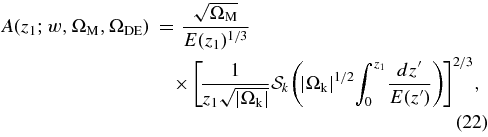
where the SDSS LRG BAO constraint is given by

with the effective LRG redshift z1 = 0.35. The second constraint is from the five-year results of the WMAP-5 (Komatsu et al. 2009). We use the shift parameter,
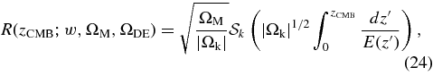
with the constraint

where zCMB is the redshift of decoupling of the CMB. Although zCMB depends upon ΩM and upon the baryon density ΩB at the ∼2% level, we fix this redshift to the WMAP-5 maximum likelihood value of zCMB = 1090 (Komatsu et al. 2009).
Minimizing χ2BAO + χ2CMB without using SNe, the best-fit cosmological parameters for the FwCDM model are w = −0.80 ± 0.20 and ΩM = 0.30 ± 0.05;41 for the ΛCDM model, ΩM = 0.27 ± 0.02 and ΩΛ = 0.74 ± 0.02. Combining these measurements with the SN samples results in improved constraints for the FwCDM model but has little impact for the ΛCDM model.
We have analyzed several different combinations of the five SN Ia data sets mentioned at the beginning of Section 5: SDSS-II, Nearby (low-redshift), ESSENCE, SNLS, and HST. In Sections 9 and 10, we present systematic uncertainties and results for the six sample combinations ((a)–(f)) shown in Table 4. Combination (a) includes only the SDSS-II SN data, without lower- or higher-redshift SNe. For combination (b), the Nearby SNe Ia are again excluded, leaving the SDSS-II SN sample to serve as the low-redshift anchor for the Hubble diagram. Combination (f) excludes the SDSS-II sample, so that we can directly compare with previously published results such as those of WV07. In combination (c), the SDSS-II serves as the "high-redshift" sample. Combination (d) includes all four ground-based samples; combination (e) includes all five samples and is used for our nominal analysis.
Table 4. Sample Combinations Used to Extract Cosmological Parameters
| Sample Combination | |
|---|---|
| (a) | SDSS-only |
| (b) | SDSS+ESSENCE+SNLS |
| (c) | Nearby+SDSS |
| (d) | Nearby+SDSS+ESSENCE+SNLS |
| (e) | Nearby+SDSS+ESSENCE+SNLS+HST |
| (f) | Nearby+ESSENCE+SNLS |
Download table as: ASCIITypeset image
8.1. Fitting Distances with mlcs2k2
As described in Section 5.1, mlcs2k2 provides an estimate of the distance modulus, μ, for each SN. Cosmological parameter estimates are derived by minimizing the following χ2 statistic (= − 2ln of the posterior probability) for the SN Ia sample over a grid of model parameter values,
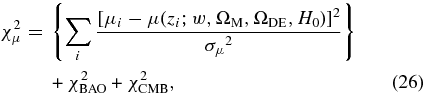
where μi is the distance modulus estimated from the mlcs2k2 fit for the ith SN, zi is its spectroscopically determined redshift, and μ(zi; w, ΩM, ΩDE, H0) = 5log(dL/10pc) is computed from Equation (20). The χ2BAO and χ2CMB terms in Equation (26) incorporate the prior information from the SDSS LRG BAO measurement (Equation (23)) and the WMAP CMB measurement (Equation (25)). When reporting values and errors on individual cosmological parameters, we use the values at the χ2μ-minimum, marginalized only over H0 (due to the degeneracy between the Hubble parameter and the fiducial peak rest-frame model magnitude). In determining w, marginalizing over ΩM shifts the value from the χ2μ-minimum by 0.025 for the SDSS-only sample and by ∼0.01 for the other sample combinations.
In Equation (26), the distance-modulus uncertainty is given by
where σfitμ is the statistical uncertainty reported by mlcs2k2, σintμ = 0.16 is the additional (intrinsic) error added so that the χ2 per degree of freedom is unity for the Hubble diagram constructed from the Nearby SN Ia sample (Section 10.1) and σzμ is calculated from the redshift uncertainty as described below.
The redshift uncertainty contains two components: from spectroscopic measurements and from peculiar motions of the host galaxy. The first source of uncertainty, σzspec, is from the uncertain redshift determination, either from the spectrum of the SN or from its host galaxy. For SDSS-II SNe we use σzspec = 0.0005 for host-galaxy-based redshifts, σzspec = 0.005 for SN-based redshifts, and the reported SDSS redshift errors for host redshifts from the SDSS spectroscopic galaxy survey (Section 3.1). For the ESSENCE and SNLS data, we use the estimated redshift errors reported in their public data tables. For the Nearby sample, redshift measurement errors were usually not reported; we take 50 km s−1 as a conservative estimate (M. Hamuy 2008, private communication). The second source of redshift uncertainty, σzspec, arises from peculiar velocities of and within host galaxies. We take σzspec = 0.0012, the quadrature sum of typical galaxy peculiar velocities of 300 km s−1 and typical internal motions of 200 km s−1. For most of the SDSS-II SNe, for which the redshift is obtained from the host galaxy, the contribution from internal motions is overestimated because these spectra are averaged over the internal galaxy motions. The final redshift uncertainty is defined to be σ2z = σ2zspec + σ2zspec. To simplify the treatment of redshift errors, we project these uncertainties onto distance modulus using the expression for the distance–redshift relation for an empty universe,
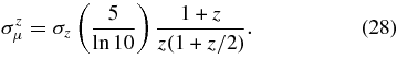
Using a different cosmological model to compute σzμ from σz leads to negligible changes in the Hubble diagram fits.
Galaxy peculiar velocities are not random, as the above treatment assumes, but are spatially correlated, since they are induced by the gravitational effects of large-scale structure. SN observations are affected by the peculiar velocities of both the host galaxies and of the Milky Way. We have accounted for the Milky Way peculiar velocity by correcting for the CMB dipole: all SN redshifts have been transformed into the comoving frame of the CMB. This is particularly important for the SDSS-II, because the equatorial stripe comes within 70 of the CMB dipole direction, and the redshift correction from the heliocentric frame is negative along the entire stripe. We use  , where z☉ is the heliocentric redshift as described in Section 3.1,
  is the unit vector pointing from the Earth to the SN, and
  is the CMB velocity vector, with a magnitude of 371 km s−1 and direction given by Galactic coordinates l = 264.140, b = +48.260 (Fixen et al. 1996). The CMB-frame redshifts for the non-SDSS-II samples are taken from the literature.
In transforming to the CMB frame and making no other corrections for velocity correlations, we are implicitly assuming that the peculiar velocities of the host galaxies are uncorrelated with that of the Milky Way and approximately uncorrelated with each other. That assumption is a good approximation for the SDSS-II and higher-redshift SN samples, which cover large spatial volumes and are distant from the Milky Way. It is not a good approximation for the Nearby SN sample on both theoretical (Hui & Greene 2006; Cooray & Caldwell 2006) and observational (Neill et al. 2007) grounds. Not including velocity correlations means that the low-redshift SNe are overweighted in the χ2μ statistic and that SN-derived cosmological parameter errors in the literature have been underestimated. However, inclusion of the SDSS-II SN sample significantly reduces the impact of the uncertainties due to low-redshift peculiar velocities.
8.2. Fitting Distances with salt-ii
In the first stage of the salt-ii analysis framework, the photometry for each SN light curve is fitted to an empirical model (Section 5.2) to determine a shape-luminosity parameter (x1), a color parameter (c), and an overall flux normalization (x0). For the salt-ii Hubble diagram analysis, the reference B-band magnitude is m*B = −2.5log [x0∫dλ'M0(t, λ')TB(λ')]. The flux integral is the same as Equation (7) with z = c = x1 = 0 and f = B. The fitted parameter x0 depends on the luminosity distance and the SN brightness.
To estimate cosmological parameters, the above parameters are related to the distance modulus for each SN by the expression

The global parameters M, α, and β describe the SN Ia population and are estimated simultaneously with the cosmological parameters by carrying out a χ2 minimization using an expression analogous to Equation (26). The minimization and error estimation are performed using the program minuit.42 The expression for the distance-modulus uncertainty, σμ, is similar to that in Equation (27) for mlcs2k2, and the redshift uncertainty is treated identically. The intrinsic dispersion (σintμ) is determined separately for each sample combination by setting the global best-fit χ2 for that sample combination to unity, in contrast to the mlcs2k2 method for which we determine σintμ solely from the Nearby sample. In addition, the salt-ii expression for χ2μ includes a covariance matrix to account for correlations between the parameters x1, c, and x0 (Section 9.2). In determining cosmological parameters, the Hubble parameter is marginalized over, but the parameters α and β are not.
If the color corrections were due only to extinction by host-galaxy dust, the salt-ii parameter β would be equal to the Cardelli et al. (1989) extinction parameter, RB (Conley et al. 2007). Further, if host-galaxy extinction were similar to the mean extinction in the Milky Way, one would expect β ≃ RB = RV + 1 ≃ 4. However, in salt-ii, β is left as a free parameter that is determined in the global fit to the Hubble diagram.
To account for selection bias, we have applied the salt-ii fitting method to simulated sample combinations (a)–(f). The Monte Carlo simulations are generated from the salt-ii model using parameters based on our analysis of the data (Section 10.2). In particular, α = 0.13 and β = 2.56, and the simulated distributions of c and x1 are described by Gaussians with  , σc = 0.13,
  ,
,  . These distributions were estimated directly from the light-curve fits rather than from simulating underlying c and x1 distributions such that the observed and simulated distributions match. The intrinsic luminosity is randomly varied using a coherent luminosity smearing factor of 0.12 mag, and the spectroscopic efficiency is based on the salt-ii parameters described in Section 6.2.1.
To isolate a potential salt-ii bias from a shift due to the CMB and BAO priors, the simulated SN sample is generated with the cosmological parameter values obtained from fitting without any SNe, w0 = −0.80 and Ω0M = 0.30. The bias in the cosmological parameters is estimated to be w − w0 and ΩM − Ω0M, where w and ΩM are obtained from the analysis of the simulated SN sample combined with the BAO+CMB priors. To increase the significance of the measured bias, 500 data-sized samples were simulated and analyzed; the resulting statistical uncertainty on the w-bias is typically 0.004. The average bias for each sample combination and cosmological model is shown in Table 5. For the results shown below in Tables 16 and 17, these bias corrections have been added to the cosmological parameters.
Table 5. salt-ii Corrections to Cosmological Parameters Based on Simulations
| Sample | FwCDM | ΛCDM | ||
|---|---|---|---|---|
| Combinationa | δw | δΩM | δΩΛ | δΩM |
| (a) | −0.04 | −0.010 | 0.001 | −0.001 |
| (b) | −0.02 | −0.007 | −0.003 | 0.004 |
| (c) | −0.02 | −0.005 | 0.001 | −0.001 |
| (d) | 0.00 | 0.006 | −0.006 | 0.007 |
| (e) | 0.00 | 0.001 | −0.008 | 0.005 |
| (f) | 0.02 | 0.006 | −0.004 | 0.005 |
Note. a(a)–(f) are defined in Table 4.
Download table as: ASCIITypeset image
9. SYSTEMATIC UNCERTAINTIES
The likelihood analysis described in the previous section accounts for the impact of statistical errors on the determination of cosmological parameters. Here, we give a detailed description of systematic uncertainties on the cosmological parameters w and ΩM within the context of the FwCDM model. For the ΛCDM model, the systematic uncertainties are evaluated in a similar fashion and are summarized along with the results in Section 10. For both mlcs2k2 and salt-ii and for each of the six sample combinations ((a)–(f)) in Table 4, we have carried out several dozen systematic tests by varying analysis parameters and methods. The resulting variations in the Hubble diagram and shifts in the parameter w (denoted by δw below) are used to assess the systematic uncertainty. To help gauge the significance of systematic shifts observed in the data, the same systematic parameter and method variations have also been applied to the analysis of Monte Carlo simulations generated with w = −1 and ΩM = 0.3, using the efficiencies determined in Section 6. There are four main categories of systematic uncertainties: (1) uncertainties in SN Ia model parameters obtained from the training procedure for the light-curve fitter; (2) uncertainties in reddening from host-galaxy dust and in intrinsic SN color variations; (3) errors in survey selection efficiencies and in associated selection biases; and (4) uncertainties in relative photometric calibration between the Nearby sample and the higher-redshift surveys.
We discuss the impact of these uncertainties in the context of the mlcs2k2 method in Section 9.1 and for the salt-ii method in Section 9.2. Summaries of the systematic uncertainties for the six sample combinations listed in Table 4 are presented in Tables 6 and 7 for mlcs2k2 and in Tables 8 and 9 for salt-ii. For the flat FwCDM model, these tables show systematic errors in the dark energy equation of state parameter w and matter density parameter ΩM, including the BAO and CMB priors discussed in Section 8. A more detailed discussion of one major source of systematic uncertainty, associated with data-model discrepancies in the rest-frame U band, is postponed to Sections 10.1.3 and 10.2.4.
Table 6. Systematic Uncertainties in Dark Energy Equation of State Parameter w for the mlcs2k2 Analysis of the FwCDM Model, Including the BAO+CMB Prior
| Uncertainty on w for Sample | ||||||
|---|---|---|---|---|---|---|
| Source of Uncertainty | (a) | (b) | (c) | (d) | (e) | (f) |
| Rest-frame U band | −0.310 | 0.080 | −0.310 | 0.080 | 0.080 | 0.080 |
| zmin cut for Nearby sample | 0.000 | 0.000 | 0.060 | 0.040 | 0.040 | 0.040 |
| mlcs2k2 SN Ia model parameters | 0.013 | 0.036 | 0.001 | 0.040 | 0.026 | 0.043 |
| Galactic extinction | 0.021 | 0.012 | 0.004 | 0.016 | 0.022 | 0.023 |
| Form of prior | ||||||
| Correlated 1σ changes RV and τV | 0.036 | 0.023 | 0.006 | 0.007 | 0.008 | 0.009 |
| Simulated efficiency for Nearby SN Ia | 0.000 | 0.000 | 0.014 | 0.008 | 0.007 | 0.013 |
| Spectroscopic efficiency for SDSS | 0.062 | 0.002 | 0.072 | 0.007 | 0.001 | 0.000 |
| Spectroscopic efficiency for ESSENCE | 0.000 | 0.013 | 0.000 | 0.012 | 0.008 | 0.012 |
| Spectroscopic efficiency for SNLS | 0.000 | 0.029 | 0.000 | 0.025 | 0.017 | 0.026 |
| Calibration | ||||||
| 0.01 mag errors in U, B, V, R, I | 0.030 | 0.029 | 0.030 | 0.021 | 0.019 | 0.021 |
| Shifted Bessell filters | 0.007 | 0.017 | 0.007 | 0.016 | 0.013 | 0.014 |
| Vary ki color terms | 0.003 | 0.007 | 0.005 | 0.006 | 0.006 | 0.006 |
| Vary SDSS AB offsets for g, r, i | 0.004 | 0.028 | 0.030 | 0.012 | 0.013 | 0.000 |
| Vary ESSENCE R − I color zero point | 0.000 | 0.011 | 0.000 | 0.015 | 0.008 | 0.010 |
| Vary SNLS g, r, i, z zero points | 0.000 | 0.040 | 0.000 | 0.036 | 0.024 | 0.035 |
| Vary HST zero points | 0.000 | 0.000 | 0.000 | 0.000 | 0.012 | 0.000 |
| Total | +0.08−0.32 | 0.11 | +0.10−0.33 | 0.11 | 0.11 | 0.12 |
Notes. Negative values indicate asymmetric uncertainties. (a) SDSS-only. (b) SDSS+ESSENCE+SNLS. (c) Nearby+SDSS. (d) Nearby+SDSS+ESSENCE+SNLS. (e) Nearby+SDSS+ESSENCE+SNLS+HST (f) Nearby+ESSENCE+SNLS.
Download table as: ASCIITypeset image
Table 7. Systematic Uncertainties in Matter Density Parameter ΩM for the mlcs2k2 Analysis of the FwCDM Model, Including the BAO+CMB Prior
| Uncertainty on ΩM for Sample | ||||||
|---|---|---|---|---|---|---|
| Source of uncertainty | (a) | (b) | (c) | (d) | (e) | (f) |
| Rest-frame U band | −0.051 | 0.016 | −0.051 | 0.016 | 0.016 | 0.016 |
| zmin cut for Nearby sample | 0.000 | 0.000 | 0.014 | 0.009 | 0.009 | 0.009 |
| mlcs2k2 SN Ia model parameters | 0.003 | 0.009 | 0.000 | 0.010 | 0.006 | 0.011 |
| Galactic extinction | 0.005 | 0.003 | 0.001 | 0.004 | 0.006 | 0.006 |
| Form of Prior | ||||||
| Correlated 1σ changes RV and τV | 0.007 | 0.006 | 0.002 | 0.002 | 0.003 | 0.002 |
| Simulated efficiency for Nearby SN Ia | 0.000 | 0.000 | 0.003 | 0.002 | 0.002 | 0.003 |
| Spectroscopic efficiency for SDSS | 0.014 | 0.001 | 0.015 | 0.002 | 0.000 | 0.000 |
| Spectroscopic efficiency for ESSENCE | 0.000 | 0.004 | 0.000 | 0.002 | 0.002 | 0.002 |
| Spectroscopic efficiency for SNLS | 0.000 | 0.008 | 0.000 | 0.007 | 0.004 | 0.007 |
| Calibration | ||||||
| 0.01 mag errors in U, B, V, R, I | 0.006 | 0.008 | 0.006 | 0.005 | 0.005 | 0.005 |
| Shifted Bessell filters | 0.001 | 0.004 | 0.001 | 0.004 | 0.003 | 0.003 |
| Vary ki color terms | 0.001 | 0.002 | 0.001 | 0.002 | 0.002 | 0.001 |
| Vary SDSS AB offsets for g, r, i | 0.001 | 0.007 | 0.006 | 0.003 | 0.003 | 0.000 |
| Vary ESSENCE R − I color zero point | 0.000 | 0.003 | 0.000 | 0.004 | 0.002 | 0.002 |
| Vary SNLS g, r, i, z zero points | 0.000 | 0.010 | 0.000 | 0.009 | 0.005 | 0.008 |
| Vary HST zero points | 0.000 | 0.000 | 0.000 | 0.000 | 0.003 | 0.000 |
| Total | +0.019−0.054 | 0.027 | +0.023−0.056 | 0.026 | 0.023 | 0.026 |
Note. Negative values indicate asymmetric uncertainties.
Download table as: ASCIITypeset image
Table 8. Systematic Uncertainties in w for the salt-ii Analysis of the FwCDM Model, Including the BAO+CMB Prior
| Uncertainty on w for Sample | ||||||
|---|---|---|---|---|---|---|
| Source of Uncertainty | (a) | (b) | (c) | (d) | (e) | (f) |
| Rest-frame U band | −0.100 | 0.104 | −0.133 | 0.104 | 0.104 | 0.104 |
| zmin cut for Nearby sample | 0.050 | 0.030 | 0.050 | 0.030 | 0.030 | 0.030 |
| Galactic extinction | 0.021 | 0.012 | 0.004 | 0.016 | 0.022 | 0.023 |
| salt-ii SN Ia model parameters | ||||||
| Retraining: include SDSS data | 0.008 | 0.005 | 0.017 | 0.011 | 0.005 | 0.005 |
| Dispersions of salt-ii surfaces | 0.001 | 0.003 | 0.002 | 0.006 | 0.006 | 0.004 |
| β-variation with redshift | 0.000 | +0.073 | 0.000 | +0.045 | +0.013 | +0.036 |
| Selection Efficiency | ||||||
| Simulated bias | 0.020 | 0.011 | 0.009 | 0.002 | 0.001 | 0.012 |
| Calibration | ||||||
| 0.01 mag errors in U, B, V, R, I | 0.029 | 0.030 | 0.027 | 0.022 | 0.020 | 0.022 |
| Shifted Bessel90 filters | 0.000 | 0.000 | 0.015 | 0.010 | 0.008 | 0.013 |
| Vary SDSS AB offsets for g, r, i | 0.018 | 0.037 | 0.031 | 0.015 | 0.016 | 0.000 |
| Vary ESSENCE R − I color zero point | 0.000 | 0.035 | 0.000 | 0.036 | 0.021 | 0.025 |
| Vary SNLS g, r, i, z zero points | 0.000 | 0.057 | 0.000 | 0.046 | 0.030 | 0.043 |
| Vary HST zero points | 0.000 | 0.000 | 0.000 | 0.000 | 0.015 | 0.000 |
| Total | +0.06−0.12 | +0.15−0.14 | +0.07−0.15 | +0.13−0.13 | +0.12−0.12 | +0.13−0.12 |
Notes. ± values indicate asymmetric uncertainties. (a) SDSS-only. (b) SDSS+ESSENCE+SNLS. (c) Nearby+SDSS. (d) Nearby+SDSS+ESSENCE+SNLS. (e) Nearby+SDSS+ESSENCE+SNLS+HST. (f) Nearby+ESSENCE+SNLS.
Download table as: ASCIITypeset image
Table 9. Systematic Uncertainties in ΩM for the salt-ii Analysis of the FwCDM Model, Including the BAO+CMB Prior
| Uncertainty on ΩM for Sample | ||||||
|---|---|---|---|---|---|---|
| Source of Uncertainty | (a) | (b) | (c) | (d) | (e) | (f) |
| Rest-frame U band | −0.020 | 0.022 | −0.024 | 0.022 | 0.022 | 0.022 |
| zmin cut for Nearby sample | 0.012 | 0.007 | 0.012 | 0.007 | 0.007 | 0.007 |
| Galactic extinction | 0.005 | 0.003 | 0.001 | 0.004 | 0.006 | 0.006 |
| salt-ii SN Ia Model parameters | ||||||
| Retraining: include SDSS data | 0.002 | 0.001 | 0.003 | 0.001 | 0.002 | 0.001 |
| Dispersions of salt-ii surfaces | 0.000 | 0.001 | 0.000 | 0.001 | 0.001 | 0.001 |
| β-variation with redshift | 0.000 | +0.016 | 0.000 | +0.010 | +0.002 | +0.007 |
| Selection efficiency | ||||||
| Simulated bias | 0.005 | 0.003 | 0.002 | 0.003 | 0.000 | 0.003 |
| Calibration | ||||||
| 0.01 mag errors in U, B, V, R, I | 0.006 | 0.008 | 0.005 | 0.005 | 0.005 | 0.005 |
| Shifted Bessel90 filters | 0.000 | 0.000 | 0.003 | 0.002 | 0.001 | 0.002 |
| Vary SDSS AB offsets for g, r, i | 0.004 | 0.007 | 0.006 | 0.003 | 0.003 | 0.000 |
| Vary ESSENCE R − I color zero point | 0.000 | 0.006 | 0.000 | 0.006 | 0.003 | 0.004 |
| Vary SNLS g, r, i, z zero points | 0.000 | 0.011 | 0.000 | 0.009 | 0.005 | 0.008 |
| Vary HST zero points | 0.000 | 0.000 | 0.000 | 0.000 | 0.003 | 0.000 |
| Total | +0.015−0.025 | +0.033−0.029 | +0.015−0.029 | +0.028−0.027 | +0.025−0.025 | +0.027−0.026 |
Note. ± values indicate asymmetric uncertainties.
Download table as: ASCIITypeset image
9.1. Systematic Uncertainties with mlcs2k2
Rest-frame U band. As discussed in detail in Section 10.1.3, there are systematic discrepancies between the mlcs2k2 rest-frame U-band model and the light-curve data for all but the Nearby SN Ia sample. We have therefore carried out a test in which the observer-frame filter corresponding to rest-frame U band is excluded from the light-curve fits and the resulting distance estimates. Figure 30 shows that for the SDSS-only sample, the exclusion of the U band causes a mean systematic shift in estimated distance modulus of 0.12 ± 0.02 mag for z > 0.21. The resulting tilt in the Hubble diagram leads to a systematic change of −0.310 in the equation of state parameter w for both the SDSS-only (a) and Nearby+SDSS (c) sample combinations; we include this shift as an asymmetric systematic uncertainty, as indicated by the minus signs in the first row of Tables 6 and 7.
For the other sample combinations ((b), (d), (e), (f)), which include the ESSENCE and SNLS samples, the exclusion of the U band results in w-shifts of 0.04–0.08. Based on tests with simulations, we cannot distinguish these shifts from random fluctuations; we therefore include the largest shift, δw = 0.08, as a symmetric systematic uncertainty for these four sample combinations.
Minimum redshift for Nearby SN sample. As discussed in Section 4, the choice of minimum redshift zmin for the Nearby sample is complicated by the so-called Hubble bubble, a jump in estimated SN Ia distance modulus around z ∼ 0.025 within the Nearby sample (JRK07). This shift is shown in the residual Hubble diagram in Figure 20, which compares the fitted SN distance modulus in redshift bins, μfit(z), with the calculated distance modulus (μcalc(z)) for a cosmological model with w = −1 and ΩM = 0.3. Since μcalc(z) is a smooth function of redshift, the jump between the two leftmost points in the plot reflects a ≃0.12 mag discontinuity in SN distance modulus (μfit(z)) at z ≃ 0.025. The significance of the shift in μ between SNe at z < 0.025 and z > 0.025 is 2.4σ. JRK07 found a comparable shift, corresponding to 0.14 mag. To further explore this issue, we also show the same residuals for the lower-redshift portion of the SDSS-II sample. The fitted SDSS-II SN distances are consistent with those of the z > 0.025 subset of the Nearby SNe Ia and less consistent with the z < 0.025 subset (∼2.5σ discrepancy).
Figure 20. Difference between fitted mlcs2k2 SN distance modulus for low-redshift SNe, μfit(z), and the calculated distance modulus μcalc(z) for a w = −1, ΩM = 0.3 model. The residuals are averaged in redshift bins of width 0.02 for the Nearby sample (black squares) and in bins of width 0.037 for the nearer portion of the SDSS-II sample (red circles). Errors are computed from  , where 0.16 is the typical magnitude dispersion per SN and N is the number of SNe in a given redshift bin. The dotted lines indicate the uncertainty in μcalc(z) resulting from an uncertainty in w of 0.15. The vertical arrow at z = 0.025 indicates the redshift associated with the Hubble bubble in JRK07.
Download figure:
Standard image High-resolution imageThe Hubble bubble may be a real feature due to a local, large-scale void, an artifact of selection biases in the Nearby SN sample, or an artifact of the light-curve fitter assumptions about host-galaxy dust and color variations. Regardless of its interpretation, this feature has been used as an argument to discard SN Ia measurements at z < 0.025 from cosmological fits (e.g., Riess et al. 2007). We have decided to make a more agnostic choice for zmin. We carry out cosmological fits using two sample combinations, Nearby+SDSS ((c)) and Nearby+SDSS+ESSENCE+SNLS (d), and vary zmin from 0.015 to 0.03; for mlcs2k2, the resulting variation in w is shown in the first two panels of Figure 21. For both sample combinations, the approximate midpoint of the w-variation occurs at zmin = 0.02, which we therefore take as the nominal choice. As zmin is varied around this value, the w-variations are approximately ±0.060 for sample combination (c) and ±0.040 for (d); we include these variations as systematic uncertainties in Table 6, with associated results for ΩM in Table 7.
Figure 21. Variation in dark energy equation of state parameter w with minimum redshift zmin as the latter is varied around the nominal value of zmin = 0.02 (shown by dotted vertical line). The fitting method (mlcs2k2 or salt-ii) and sample combination are indicated in each panel.
Download figure:
Standard image High-resolution imagemlcs2k2 SN Ia model parameters. The mlcs2k2 model vectors M, p, and q in Equation (1) were determined by training the light-curve fitter on a Nearby SN Ia sample, as described in JRK07. As discussed in Section 5.1, our analysis uses a set of model vectors that includes the adjustments to the  values given in Equation (2). To estimate the sensitivity of the results to these adjustments, we have also carried out the cosmology analysis using the mlcs2k2 model vectors without those adjustments. These two sets of model vectors result in values for w that differ by δw = 0.01–0.04, depending on the sample combination.
Galactic extinction. The wavelength dependence of the Milky Way Galactic extinction is expressed as A(λ) = AV × (a(λ) + b(λ)/RV), where RV = 3.1, AV = RV × E(B − V), E(B − V) is the color excess, and the functions a(λ) and b(λ) are defined by Cardelli et al. (1989). To estimate the systematic uncertainty for each SN, we coherently decrease the color excess by 0.01 + 0.16 × E(B − V) mag (but requiring non-negative color excess) relative to the nominal value in Schlegel et al. (1998). The color-excess uncertainty of 0.01 mag is based on optical-versus-IR discrepancies (Burstein 2003). The resulting w-uncertainties are 0.01–0.02. Note that we have not varied the functions a(λ) and b(λ), and therefore this uncertainty may be underestimated. The mean Galactic extinctions in the r band are 0.20 (Nearby), 0.14 (SDSS), 0.07 (ESSENCE), 0.05 (SNLS) and 0.01 mag (HST).
Dust parameter RV. As described in Section 7.1, the SDSS dust sample was used to determine the dust reddening parameter, RV = 2.18 ± 0.50 (Section 7.2), and the extinction distribution exponential slope, τV = 0.334 ± 0.088 (Section 7.1). Propagating the correlated uncertainties on RV and τV, the uncertainty on w is δw = 0.036 for the SDSS-only sample. For the combined data samples, δw ≲ 0.03. This color-related uncertainty appears rather small, considering that the issue of color variations has been a major source of uncertainty in previous studies such as WV07.
Simulated spectroscopic efficiency. The simulated efficiency is part of the mlcs2k2 fitting prior, as indicated by the terms search and cuts in Equation (5). The main effect of an error in determining the spectroscopic efficiency is to introduce a bias in the mlcs2k2 prior (Equation (5)). As discussed in Section 6, the largest uncertainty in simulating the efficiency is related to modeling of the incompleteness of the spectroscopic observations, spec.
For the Nearby, SDSS, and SNLS samples, spec depends mainly on the  component, i.e.,
  in Section 6.2.1. We explore the systematic error due to spectroscopic efficiency modeling for these samples by repeating the analysis with spec set to unity, an extreme variation from the fiducial efficiency model of Section 6.2.1. Since the ESSENCE sample favors a purely redshift-dependent spec (
 in Equation (14)), setting spec = 1 has no impact in that case; we instead evaluate the systematic error for that sample by replacing the purely z-dependent spec with a purely
  -dependent spec, i.e., by setting
  . In these tests, the efficiency due to photometric selection cuts (cuts) is included in the fitting prior as well as the image-subtraction efficiency (subtr) for the SDSS sample.
For the above systematic changes in spec, the corresponding changes in distance modulus versus redshift are shown in Figure 22 for both the data and the Monte Carlo simulations. One clearly sees that incorporating a non-trivial spectroscopic efficiency model has a significant systematic impact on distance estimates for the more distant SNe in each sample. Moreover, the data-simulation agreement is good, adding confidence in our implementation of the spectroscopic efficiency model in the fitting prior.

Figure 22. Systematic impact of uncertainty in the spectroscopic efficiency model for different samples. Upper panels: data samples; lower panels: simulated samples. For each sample, the difference in distance modulus between using an extreme spectroscopic efficiency model (μ(systspec)) and using the fiducial efficiency model (μ) is shown vs. redshift. For the Nearby, SDSS, and SNLS data sets, the extreme model assumes no spectroscopic incompleteness (spec = 1). For ESSENCE, the extreme model assumes pure Malmquist-induced incompleteness, and the negative of the μ-difference is plotted instead in order to better compare with the results for the other samples. The simulated samples have 2.5 times more points than the data samples for enhanced statistics. The differences in μ appear only for z > zcut as explained in Section 6.2.1.
Download figure:
Standard image High-resolution imageFrom Figure 9, there is no doubt that spec is significantly less than one and that our model for spec is closer to reality than the extreme assumption of setting spec = 1. To be conservative, we use half of the absolute-value difference in w between the fiducial and extreme efficiency models as our estimate of the systematic error associated with uncertainty in the efficiency model. The largest uncertainty related to the simulated efficiency occurs for sample combinations (a) and (c); the w-uncertainties (half the shifts) are δw = 0.062 for the SDSS-only sample and δw = 0.072 for the Nearby+SDSS sample combination (c). We also note that including versus not including the simulated efficiency in the Nearby SN sample changes w by a few hundredths for the other sample combinations that include the Nearby sample, half of which is included as a systematic uncertainty.
Calibration of the primary reference star, BD+17. As discussed in Appendix B, the UBVRI magnitudes of the primary spectrophotometric reference star, BD+17, are used in the K-corrections to relate the flux calibration of the Nearby SN sample to that of the higher-redshift samples. To evaluate the uncertainty in the BD+17 magnitudes, we compare the consistency of the synthetic magnitudes of the HST spectra with the SDSS photometric magnitudes. We first compute u, g, r, i, z zero-point offsets as the difference between synthetic BD+17 magnitudes computed from the HST-measured spectrum (Bohlin 2007) and the magnitudes measured by Landolt (2007). These offsets are then compared to those based on three solar analogs (P3330E, P177D, P041C). The differences between the zero-points offsets are −0.004, −0.013, 0.005, 0.010, 0.012 mag for u, g, r, i, z, respectively. We therefore assume a 1% uncertainty in each of the U, B, V, R, I magnitudes for BD+17. To propagate this error, we change each BD+17 magnitude by 1% independently in each passband; for each change, all of the SN light curves are re-fitted with the mlcs2k2 model and cosmological parameters are extracted. The resulting five independent w-shifts are then added in quadrature and included as a systematic uncertainty. The resulting w-uncertainties are 0.02–0.03.
As a crosscheck, we have replaced BD+17 with Vega as the primary reference star. The resulting changes in w are consistent with the changes from applying 1% shifts in the U, B, V, R, I magnitudes of BD+17. The differences between BD+17 and Vega are therefore not included as a systematic uncertainty.
Landolt–Bessell color transformations. As discussed in Appendix B, we use color transformations to transform between the Landolt network and the filter system defined by Bessell (1990). Table 20 shows the color terms (ki) between Landolt magnitudes and synthetic magnitudes using the Bessell (1990) filters. We vary each color term independently by one standard deviation, and the corresponding changes in w are added in quadrature. The resulting change is δw < 0.01 for all sample combinations.
Shifted Bessell filters instead of color transformation. As an alternative to the Landolt–Bessell color transformation, we consider the approach of Astier et al. (2006), using a modified set of UBVRI filter responses in which the shapes of the Bessell (1990) response curves are held fixed, but the central wavelength of each filter passband is shifted so that the color terms (Equation (B2)) are zero. The corresponding wavelength shifts are given in Table 21 under the column "HST standards." Using these wavelength shifts and no color transformations in place of the color transformation method of Appendix B, w shifts by δw = 0.007 for the SDSS-only sample. For the other sample combinations, δw ∼ 0.01.
SDSS AB offsets. As discussed in Section 3.2, the uncertainties in the SDSS AB offsets are 0.009, 0.009, 0.009 mag for g, r, i, respectively (see Table 1). These uncertainties include zero-point uncertainties of 0.004, 0.004, 0.007 mag based solely on the consistency of the solar analogs and also account for uncertainties in the central wavelengths of the SDSS filters: δλ ≃ 7, 16, 25 Å for g, r, i, respectively. We independently vary each AB offset by one standard deviation, and the resulting changes in w are added in quadrature. The resulting change in w is a few hundredths for the sample combinations that include SDSS-II SNe. Note that the w-uncertainty for SDSS-only (δw = 0.004) is much smaller than that for the Nearby+SDSS combination (δw = 0.030). For SDSS-only, the effect of changing the AB offsets is mainly to shift all of the distance moduli by the same amount; the corresponding change in cosmological parameters is small. For Nearby+SDSS, the SDSS-II distances are shifted relative to those of the Nearby sample, and the abrupt feature in the Hubble diagram results in a larger change in the cosmological parameters.
ESSENCE R −I color zero point. WV07 report an uncertainty of 0.02 mag in their R − I color zero point, resulting in a systematic uncertainty of δw = 0.04 for their analysis of the Nearby+ESSENCE data sets. As a crosscheck, we propagate their R − I uncertainty into our analysis and find δw = 0.05 for the same Nearby+ESSENCE combination, in reasonable agreement with WV07. We apply their R − I uncertainty to our sample combinations and find that the uncertainty in w is much smaller, δw ∼ 0.01 for the combinations ((b), (d), (e), (f)) that include the ESSENCE sample. Note that these sample combinations also include the SNLS sample, suggesting that the impact of the ESSENCE R − I uncertainty is reduced by the presence of another high-redshift data sample.
SNLS g, r, i, z zero points. Astier et al. (2006) reported zero-point uncertainties of 0.01, 0.01, 0.01, 0.03 for their g, r, i, z passbands, respectively. In their analysis of the Nearby+SNLS combination, they vary each zero point independently and add the corresponding w-shifts in quadrature: the resulting systematic is δw = 0.05. As a crosscheck, we propagate their zero-point uncertainties into our analysis and also find δw = 0.05 for the same Nearby+SNLS combination. We apply their zero-point uncertainties to our sample combinations and find slightly smaller uncertainties for the combinations ((b), (d), (e), (f)) that include the SNLS sample.
HST zero points. The HST zero-point uncertainties are 0.02 mag for the F110W and F160W filters43 (mean wavelengths are 1.14 μm and 1.61 μm, respectively), and 0.01 mag for the optical filters.44 For the analysis of the five-sample combination that includes HST (e), the resulting w-uncertainty is δw = 0.012.
The cosmological parameter shifts due to all of these sources of systematic error are added in quadrature to derive total systematic-error estimates δw and δΩM for the mlcs2k2 analysis of the FwCDM model; these are given in Tables 6 and 7.
9.2. Systematics Uncertainties with salt-ii
To examine systematic uncertainties in the context of the salt-ii model, we undertake an analysis similar to that carried out for mlcs2k2. We also determine systematic uncertainties for the salt-ii parameters α and β that enter Equation (29). Since the salt-ii training software is not available for public use, with one exception we make approximations in cases where re-training of the spectral surfaces is needed. In such cases we either use the nominal salt-ii surfaces and propagate changes only in the light-curve fits, or we use the uncertainties based on the mlcs2k2 analysis. The systematic uncertainties in w and ΩM for the different sample combinations are given in Tables 8 and 9.
Rest-frame U band. As discussed in detail in Section 10.2.4, there are systematic discrepancies between the salt-ii rest-frame U-band model and the observer-frame U-band light-curve data for the Nearby SN Ia sample. As was noted in Section 9.1, a related issue is seen for mlcs2k2. We carry out a test of the salt-ii fits in which the observer-frame filter corresponding to the rest-frame U band is excluded from the fits. Figure 40 shows that for the SDSS-only sample, the exclusion of the U band results in a redshift-dependent change in the distance modulus. This results in a w-shift of −0.100 for the SDSS-only sample and −0.133 for the Nearby+SDSS combination; these shifts are included as asymmetric systematic uncertainties.
For the other sample combinations, which include the higher-redshift ESSENCE and SNLS samples ((b),(d),(e),(f)), the exclusion of the rest-frame U band results in w-shifts of 0.04–0.09. Based on tests with simulations, we cannot distinguish these shifts from random fluctuations; we therefore include the largest shift, δw = 0.09, as a symmetric systematic uncertainty for these four sample combinations. If the observer-frame U band is excluded from the Nearby sample, while the rest-frame U band is included in the higher-redshift samples, the change in w is no more than 0.01.
Minimum redshift for Nearby SN sample. The dependence of the salt-ii results for w on the zmin cut is shown in the third and fourth panels of Figure 21. For zmin ≳ 0.018, the inferred value of w is fairly insensitive to the value of zmin. However, when zmin is reduced to 0.015, w changes by almost 0.09 for the Nearby+SDSS combination, and by 0.04–0.05 for the combinations that include the higher-redshift (ESSENCE and SNLS) samples. To account for these variations, we have assigned a systematic uncertainty of δw = 0.05 for the Nearby+SDSS combination and δw = 0.03 for the other sample combinations that include the Nearby SN Ia sample.
Galactic extinction. The systematic uncertainty from Galactic extinction is described in Section 9.1, resulting in δw ∼ 0.02.
salt-ii training with SDSS-II data. Here we examine the salt-ii training process that produces the spectral surfaces M0(t, λ) and M1(t, λ) in Equation (6). Because SDSS-II SN probes a relatively unexplored range of SN redshifts, the rest-frame behavior of the SDSS-II light curves may not be as well described by the salt-ii model as that of other SN samples that were used in the training of the model. To quantify this issue, J. Guy has retrained the salt-ii spectral surfaces twice, first including the light curves of the SDSS spectroscopic sample and second including those of the SDSS dust sample (Section 7.1). Evaluating cosmological parameters obtained with each retrained set of spectral surfaces and comparing the results with those from the standard salt-ii training, we include the larger of the two w-shifts as a systematic uncertainty. For the SDSS-only and Nearby+SDSS ((a) and (c)) sample combinations, the uncertainty is δw ∼ 0.02. For the other combinations, δw ∼ 0.01.
salt-ii dispersions. Recall from Section 5.2 that the spectral surfaces, M0(t, λ) and M1(t, λ), were retrained using the Bessell filter shifts based on HST standards (Table 21). The model dispersions around these surfaces, however, were not determined in the retraining, and we therefore use the model dispersions from Guy et al. (2007). To allow for the resulting uncertainty in the dispersions, we assign a systematic uncertainty of half the difference between using and ignoring the dispersions. The resulting uncertainties are δw ∼ 0.01–0.02 for combinations that include the higher-redshift ESSENCE and SNLS samples. For the SDSS-only and Nearby+SDSS sample combinations, the w-uncertainty is negligible.
β-variation with redshift. If the salt-ii SN parameters (α, β, M) are allowed to vary independently in redshift bins, while the cosmological parameters are fixed, we find a strong redshift dependence of β for z > 0.6 (see Section 10.2.3). To estimate the corresponding systematic uncertainty, the Hubble diagram fits have been redone allowing α, β, and M to vary with redshift using a simple model in which each SN parameter is constant for z < 0.6, and is then allowed to vary linearly with redshift for z > 0.6. Compared to the nominal salt-ii model with redshift-independent parameters, the largest change, δw = +0.073, occurs for SDSS+ESSENCE+SNLS (b) in which the Nearby sample is excluded. For sample combinations (d) and (f), δw ∼ 0.04, and for the full SN set (e) that includes the HST, δw ∼ 0.01. These w-shifts are included as asymmetric systematic uncertainties.
Simulated bias correction. For salt-ii, we have determined bias corrections from simulations, as described in Section 8.2 (see Table 5). We include half the w-shift as a systematic uncertainty. The largest uncertainty is δw = 0.020 for SDSS-only.
Calibration of primary reference star, Vega. We assume uncertainties of 0.01 mag in the calibration of U, B, V, R, I for the primary reference, Vega. Since a full accounting of this effect would require another retraining of the salt-ii surfaces, we instead adopt the uncertainties derived from the mlcs2k2 analysis (Table 6). In Astier et al. (2006), the corresponding uncertainty is δw = 0.024 for the Nearby+SNLS combination; as a crosscheck, we have evaluated this uncertainty for the same sample combination and find good agreement, δw ≃ 0.021. For the sample combinations analyzed here, the resulting w-uncertainties are 0.02–0.03.
Calibration: shifted Bessell filters for Nearby data. As discussed in Section 5.2, we use the Bessell (1990) filter responses with wavelength shifts given in Table 21 of Appendix B. Since these shifts differ from those in Astier et al. (2006), we use the difference in cosmological results derived from both sets of wavelength shifts to define an additional systematic uncertainty on w. This uncertainty is δw ∼ 0.02 for sample combinations that include the Nearby sample.
Calibration: zero-point offsets for SDSS, ESSENCE, SNLS, HST. Zero-point uncertainties for the SDSS, ESSENCE, SNLS, and HST bandpasses are propagated in the same manner as for the mlcs2k2 method (Section 9.1). The SNLS zero points are varied in the fit, but not in the training of the spectral surface, and therefore these w-uncertainties might be slightly overestimated. The other survey samples were not used in the training, and therefore varying the zero points in the fit is sufficient to estimate the systematic error. Note that the w-uncertainty from the SDSS AB offsets is smaller for SDSS-only than for Nearby+SDSS, as explained in Section 9.1.
The parameter shifts due to all of these systematic errors are added in quadrature to derive the total systematic-error estimates in Tables 8 and 9.
10. RESULTS
Here we present the Hubble diagram and inferred cosmological parameters using the framework described in Section 8. Results based on the mlcs2k2 and salt-ii methods are presented in Sections 10.1 and 10.2, respectively. We compare the results from the two methods in Section 11.
The Hubble diagram for the five samples considered in this analysis is shown in Figure 23. The distance moduli here are obtained from the mlcs2k2 method described above; the Hubble diagram based on the salt-ii method looks quite similar. Detailed Hubble-residual plots are given for each method in Sections 10.1 and 10.2.
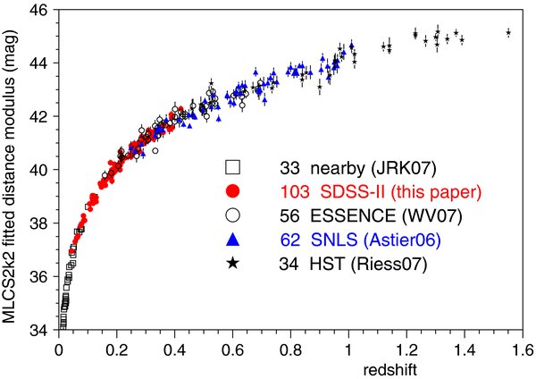
Figure 23. Fitted distance modulus (from mlcs2k2) vs. redshift for the 288 SNe Ia from the five samples indicated on the plot.
Download figure:
Standard image High-resolution image10.1. Results with mlcs2k2
Using the mlcs2k2 method, we present cosmological results for the six sample combinations (a)–(f) of Table 4. Table 10 shows the spectroscopically determined redshift and marginalized mlcs2k2 fit parameters for SNe that pass the selection cuts described in Section 4. We use the ensemble of redshifts zi and estimated distance moduli μi for each sample combination to fit cosmological model parameters, as explained in Section 8.1.
Table 10. Parameters from mlcs2k2 Light-Curve Fits (Uncertainties in Parentheses)
| SNID | Redshifta | μ | AV | Δ | MJDpeak |
|---|---|---|---|---|---|
| 762 | 0.1904(.0001) | 40.05(0.10) | 0.20(0.08) | −0.22(0.07) | 53624.4(0.4) |
| 1032 | 0.1291(.0002) | 38.80(0.10) | 0.07(0.06) | 0.88(0.09) | 53626.9(0.2) |
| 1112 | 0.2565(.0002) | 40.84(0.18) | 0.13(0.09) | 0.05(0.16) | 53629.3(1.0) |
| 1166 | 0.3813(.0005) | 41.51(0.18) | 0.16(0.11) | −0.25(0.13) | 53630.1(1.1) |
| 1241 | 0.0858(.0050) | 38.10(0.09) | 0.40(0.06) | 0.02(0.06) | 53634.7(0.2) |
| 1253 | 0.2609(.0050) | 40.65(0.14) | 0.06(0.05) | 0.08(0.12) | 53634.2(0.5) |
Notes. The complete table for all 288 SNe is given in the online journal, and also at http://das.sdss.org/va/SNcosmology/sncosm09_fits.tar.gz. aSpectroscopic redshift in CMB frame.
Only a portion of this table is shown here to demonstrate its form and content. A machine-readable version of the full table is available.
Download table as: DataTypeset image
10.1.1. Goodness of Fit and Hubble Scatter
Before considering the cosmological parameter results for the various combined samples, we examine several measures of fit quality and dispersion for each SN Ia sample treated independently, since they provide diagnostic information that is useful to consider before combining the samples. Table 11 displays these measures: (1) the χ2μ statistic for the best-fit FwCDM model for that sample from Equation (26)—in goodness-of-fit tests, this statistic is usually compared to the number of degrees of freedom, given by Ndof = NSN − 1;45 (2) the root-mean-square (rms) measure of Hubble scatter,  , where μi is the estimated distance modulus from the light-curve fit for the ith SN, and μfiti is the best-fit FwCDM model distance modulus at the corresponding redshift zi; and (3) the value of σintμ that would be required in Equation (27) to make χ2μ = Ndof in Equation (26) for that sample. In computing the first two measures, we adopt σintμ = 0.16, the value that yields χ2μ = Ndof for the Nearby SN sample and that we use in analyzing the combined samples, as explained in Section 8.1. The bottom row of Table 11 shows the χ2μ statistic from the SNe in each sample when the best-fit FwCDM model parameters for the global sample combination Nearby+SDSS+ESSENCE+SNLS+HST (e) are used to determine μfiti. Compared to the values for the independent fits to each sample, the χ2μ values for the global fit are only slightly larger. For the Nearby, ESSENCE, SNLS, and HST samples, the reduced statistic, χ2μ/Ndof, is close to unity, and rmsμ = 0.19 to 0.28 mag. For the SDSS-II sample, the reduced χ2μ/Ndof ∼ 0.5, and rmsμ = 0.15, both substantially smaller than for the other samples.
Table 11. Hubble Diagram Fit-Quality Parameters Using mlcs2k2 Distances
| Result for Sample | |||||
|---|---|---|---|---|---|
| Fit-Quality Parameter | Nearby | SDSS | ESSENCE | SNLS | HST |
| χ2μ | 31.9 | 55.3 | 46.8 | 63.0 | 32.5 |
| Ndof | 32 | 102 | 55 | 61 | 33 |
| rmsμ | 0.19 | 0.15 | 0.23 | 0.24 | 0.28 |
| σintμ (χ2μ = Ndof) | 0.16 | 0.09 | 0.13 | 0.16 | 0.15 |
| χ2μ (global fit) | 32.9 | 56.6 | 48.4 | 64.6 | 32.4 |
Download table as: ASCIITypeset image
We attribute the smaller scatter and χ2μ of the SDSS-II sample largely to spectroscopic selection effects. As described in Section 2, when prioritizing candidate SNe for spectroscopic observations, preference was given to those that were far from host-galaxy cores and/or that were hosted by redder (and presumably less dusty) galaxies. In Appendix E, this explanation is quantified by comparing the Hubble scatter and χ2μ statistic for the spectroscopic SN Ia sample to those for the host-z sample of photometrically identified SNe Ia that have spectroscopic redshifts from subsequent host-galaxy observations. The cosmology analysis accounts for this selection effect via the model for the search efficiency (Section 6.2.1) in the mlcs2k2 fitting prior and by including a systematic error that reflects uncertainties in the search efficiency.
10.1.2. mlcs2k2 Hubble Diagrams and Cosmological Parameters
Figure 24 shows the differences between the estimated SN distance moduli μi and those for an open CDM model with no dark energy (ΩM = 0.3, ΩDE = 0) as a function of redshift, for each of the six SN sample combinations; the large square (pink) points show weighted averages of these residuals in redshift bins. Also shown is the Hubble distance-residual curve between the best-fit FwCDM model for each sample combination (including the BAO+CMB prior) and that for the open model (solid curves). In each panel, the Hubble parameter for the open CDM model has been adjusted to agree with that for the best-fit FwCDM model, so that the FwCDM versus open CDM residuals vanish at z = 0. Since the Hubble parameter is not determined in this analysis, a constant vertical offset in Figure 24 is irrelevant: what is significant are the slope and curvature of the points and the best-fit (solid) curves versus redshift. Figure 25 shows the distributions of normalized residuals, (μi − μFwCDM)/σμ, where μFwCDM is the distance modulus from the best-fit FwCDM model for sample combination (e) including the BAO+CMB prior, and σμ is the total uncertainty defined in Equation (27). The bulk of the distribution of all 288 normalized residuals (the upper left panel of Figure 25) is well fitted by a Gaussian with σ = 0.77; outliers increase the rms to 0.90. For the Nearby sample, the rms is one as expected, because σintμ = 0.16 mag is determined such that χ2μ/Ndof = 1.
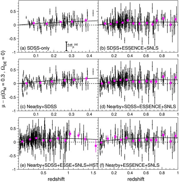
Figure 24. Hubble residuals for the mlcs2k2 method: differences between measured SN distance moduli and those for an open CDM model (ΩM = 0.3, ΩDE = 0) vs. redshift for the six SN sample combinations. Large, square (pink) points show weighted averages in redshift bins: within each redshift bin, the points are plotted at the weighted mean redshift given by  , where σi is the distance-modulus uncertainty. Solid curves show the difference between the best-fit FwCDM model distance modulus and that for the open model, normalized to have the same value of the Hubble parameter. The error bars on the data points correspond to the distance-modulus error σfitμ from the mlcs2k2 light-curve fit (Equation (27)), i.e., they do not include the intrinsic scatter or the effects of redshift and peculiar velocity errors. The vertical bar in panel (a) shows the intrinsic uncertainty, σintμ = 0.16, included in the cosmology fits so that the χ2 per degree of freedom is unity for the Hubble diagram constructed from the Nearby SN Ia sample alone.
Download figure:
Standard image High-resolution image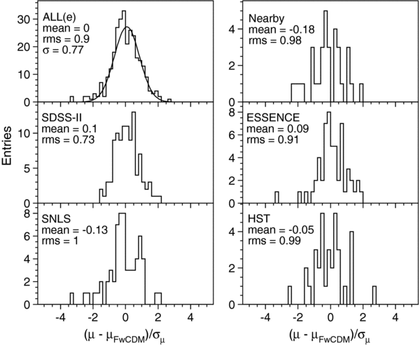
Figure 25. Distribution of normalized Hubble residuals (pull) for the mlcs2k2 method, for the Nearby+SDSS+ESSENCE+SNLS+HST sample combination (e) (upper left, along with the Gaussian fit) and for each SN sample indicated on the plots. μ is the measured SN distance modulus, μFwCDM is the distance modulus from the best-fit FwCDM model (for sample combination (e)) at the same redshift, and σμ is the total uncertainty (Equation (27)). The mean and rms for each distribution are indicated on each panel.
Download figure:
Standard image High-resolution imageFigures 26 and 27 show the mlcs2k2 statistical-uncertainty contours for the FwCDM and ΛCDM models: for each of the six sample combinations, the SN Ia, BAO, and CMB contours are shown along with the combined constraints. For the combined SN+BAO+CMB results, we include systematic uncertainties to derive total (statistical plus systematic) uncertainty contours, as explained in Appendix F, with results shown in Figures 28 and 29 for the FwCDM and ΛCDM models (note the zoomed axis scales compared to the previous figures). The best-fit cosmological parameter values and uncertainties, including the BAO and CMB priors, are given in Tables 12 and 13 for the FwCDM and ΛCDM models. The distance modulus versus redshift curve for the best-fit FwCDM cosmological parameter values (relative to that of an open CDM model) are shown as the solid curves in the Hubble residual plots in Figure 24.

Figure 26. For the FwCDM model, mlcs2k2 statistical-uncertainty contours in the ΩM–w plane for each of the six SN sample combinations indicated on the plots. Shaded regions: 68% and 95% confidence level regions for the SN data alone; green: corresponding CL contours for SDSS BAO (Eisenstein et al. 2005); blue: CL contours for WMAP-5 CMB (Komatsu et al. 2009); closed, black contours: combined constraints from SN+BAO+CMB.
Download figure:
Standard image High-resolution image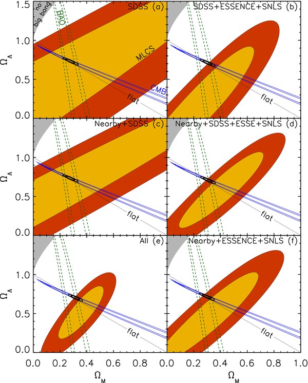
Figure 27. For the ΛCDM model, mlcs2k2 statistical-uncertainty contours in the ΩM–ΩΛ plane for each of the six SN sample combinations indicated on the plots. Shaded regions: 68% and 95% confidence level regions for the SN data alone; green: corresponding CL contours for SDSS BAO; blue: CL contours for WMAP-5 CMB; closed, black contours: combined constraints from SN+BAO+CMB. The gray region indicates models with no big bang, i.e., with a bounce at a finite value of the FRW scale factor. The solid diagonal line indicates a spatially flat Universe, with ΩM + ΩΛ = 1.
Download figure:
Standard image High-resolution image
Figure 28. For mlcs2k2 and the FwCDM model, 68% CL contours in the ΩM–w plane for each of the six SN sample combinations, using the combined SN+BAO+CMB constraints. Solid contours are total (statistical+systematic) uncertainty; dashed contours are statistical only. Systematic errors have been included using the prescription in Appendix F.
Download figure:
Standard image High-resolution image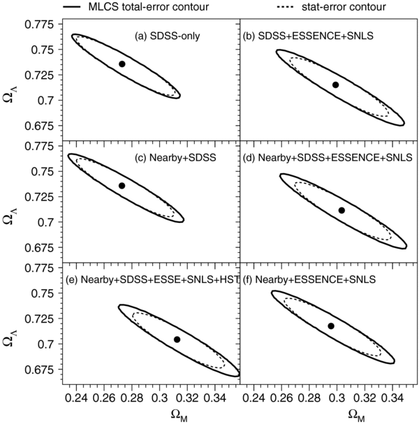
Figure 29. For mlcs2k2 and the ΛCDM model, 68% CL contours in the ΩM–ΩΛ plane for each of the six SN sample combinations, using the combined SN+BAO+CMB constraints. Solid contours are total (statistical+systematic) uncertainty; dashed contours are statistical only. Systematic errors have been included using the prescription in Appendix F.
Download figure:
Standard image High-resolution imageTable 12. For the FwCDM Model, Constraints on w and ΩM from mlcs2k2 SN Distances Combined with SDSS BAO and WMAP-5 CMB Results
| Parameter | Result for Sample Combination | |||||
|---|---|---|---|---|---|---|
| (a) | (b) | (c) | (d) | (e) | (f) | |
| χ2μ | 170.9 | 406.7 | 279.5 | 517.8 | 568.1 | 341.9 |
| Ndof | 102 | 220 | 135 | 253 | 287 | 150 |
| rmsμ | 0.15 | 0.20 | 0.16 | 0.20 | 0.21 | 0.23 |
| w | −0.84 | −0.71 | −0.92 | −0.76 | −0.76 | −0.78 |
| σw(stat) | 0.15 | 0.09 | 0.13 | 0.08 | 0.07 | 0.08 |
| σw(syst) | +0.08−0.32 | 0.11 | +0.10−0.33 | 0.11 | 0.11 | 0.12 |
| σw(tot) | +0.17−0.35 | 0.14 | +0.16−0.35 | 0.14 | 0.13 | 0.14 |
| ΩM | 0.289 | 0.319 | 0.273 | 0.306 | 0.307 | 0.302 |
 |
0.033 | 0.025 | 0.028 | 0.021 | 0.019 | 0.022 |
 |
+0.019−0.054 | 0.027 | +0.023−0.056 | 0.026 | 0.023 | 0.026 |
 |
+0.038−0.064 | 0.036 | +0.036−0.062 | 0.033 | 0.030 | 0.034 |
Notes. aSDSS-only. bSDSS+ESSENCE+SNLS. cNearby+SDSS. dNearby+SDSS+ESSENCE+SNLS. eNearby+SDSS+ESSENCE+SNLS+HST. fNearby+ESSENCE+SNLS.
Download table as: ASCIITypeset image
Table 13. For the ΛCDM Model, Constraints on ΩM and ΩΛ from mlcs2k2 SN Distances Combined with SDSS BAO and WMAP-5 CMB Results
| Parameter | Result for Sample Combination | |||||
|---|---|---|---|---|---|---|
| (a) | (b) | (c) | (d) | (e) | (f) | |
| χ2μ | 55.2 | 171.7 | 87.1 | 203.9 | 237.9 | 145.8 |
| Ndof | 102 | 220 | 135 | 253 | 287 | 150 |
| rmsμ | 0.15 | 0.20 | 0.16 | 0.20 | 0.21 | 0.23 |
| ΩΛ | 0.735 | 0.714 | 0.735 | 0.713 | 0.705 | 0.718 |
 |
0.019 | 0.019 | 0.019 | 0.019 | 0.018 | 0.019 |
 |
0.000 | 0.000 | 0.006 | 0.004 | 0.004 | 0.004 |
 |
0.019 | 0.019 | 0.019 | 0.019 | 0.018 | 0.019 |
| ΩM | 0.274 | 0.300 | 0.274 | 0.302 | 0.312 | 0.294 |
 |
0.023 | 0.023 | 0.023 | 0.023 | 0.022 | 0.023 |
 |
0.000 | 0.000 | 0.001 | 0.001 | 0.001 | 0.001 |
 |
0.023 | 0.023 | 0.023 | 0.023 | 0.022 | 0.024 |
Download table as: ASCIITypeset image
Among the six SN sample combinations, the best-fit values of the dark energy equation of state parameter w fall roughly into two groups. In the first group, the highest-redshift sample is from SDSS-II: for the SDSS-only sample (a) and Nearby+SDSS sample combination (c), w = −0.84 and −0.92. The agreement between these values is consistent with the expected rms spread of 0.07 based on simulations. The second group comprises the other four sample combinations, which include the higher-redshift ESSENCE and SNLS samples: w = −0.71, − 0.76, − 0.76, − 0.78 for sample combinations (b), (d), (e), (f), respectively. Simulations predict an rms spread in w of ∼0.1 between the results from these two groups; the observed difference is therefore not statistically significant but may nevertheless be an indicator of systematic effects.
Table 12 also shows that the statistical and systematic errors in w and ΩM for sample combinations (b) and (f) are very similar. Since these two sample combinations differ only in the substitution of the Nearby SN Ia sample with the SDSS-II sample, this indicates that the first-season SDSS-II SN sample anchors the Hubble diagram with comparable constraining power to the Nearby sample.
Using the Nearby+SDSS+ESSENCE+SNLS+HST sample combination (e), which covers the widest redshift range, we obtain w = −0.76 ± 0.07(stat) ± 0.11(syst) and ΩM = 0.307 ± 0.019(stat) ± 0.023(syst). Although this value for w is higher than that obtained from other recent SN measurements, we stress that the difference is not due to inclusion of the SDSS-II SN data: as Table 12 shows, we infer nearly identical parameter values for sample combination (f), which excludes the SDSS-II data. By contrast, WV07 inferred w = −1.07 ± 0.09(stat) ± 0.13(syst), ΩM = 0.267+0.028−0.018(stat) using mlcs2k2 for a sample combination nearly identical to (f) and including the BAO (but not CMB) constraints. In Section 10.1.4, we trace the differences between the WV07 result and ours to changes in mlcs2k2 model parameters and assumptions.
For the ΛCDM model, in comparison with the FwCDM model, the SN results carry less weight relative to the combined BAO and CMB results in constraining the parameters. In particular, Figure 27 and Table 13 show that the SDSS-only (a) and Nearby+SDSS (c) SN samples have almost no impact on the maximum likelihood parameter values and uncertainties. For the other four SN sample combinations, there is some tension between the SN and BAO results: the SN results pull the maximum likelihood parameter values along the CMB contour, away from the BAO contours. Since the BAO contours are in all cases narrower than those for the SNe, however, this shift is small, corresponding to δΩDE ≃ −0.03, δΩM ≃ 0.04 or less.
10.1.3. U-Band Anomaly with mlcs2k2
As noted in Section 9.1, the largest single contribution to the systematic-error budget comes from consideration of the rest-frame U band. Within the mlcs2k2 framework, the issue is manifest as a difference between the Nearby sample (JRK07) and the other SN Ia samples. We have carried out a series of tests in which the observer-frame passband corresponding to rest-frame U band is excluded from the mlcs2k2 light-curve fits. We compare the resulting distance-modulus estimates, μnoU, with those for which rest-frame U band is included, μ, and define ΔμnoU, ≡ μnoU − μ. If the mlcs2k2 model is a good description of the data, we would expect ΔμnoU, to scatter about zero.
The left panel of Figure 30 shows the resulting change in the SDSS-II SN Hubble diagram, ΔμnoU, versus redshift. For z > 0.21, observer-frame g corresponds to rest-frame U; excluding g band in this redshift range results in a shift in the distance modulus of ΔμnoU, = (0.12 ± 0.02) mag. In the redshift interval 0.21 < z < 0.285, the remaining observer-frame SDSS passbands r and i correspond to rest-frame V and R; for z > 0.285, they correspond to B and V. In both of those redshift intervals, we see a distance-modulus shift of ΔμnoU, ≃ 0.1–0.15 mag. For z < 0.21, the gri filters do not map onto rest-frame U band, therefore ΔμnoU, ≡ 0 in this redshift range. Since ΔμnoU, is determined from strongly correlated samples, i.e., the r- and i-band data are the same in fits with and without U band, its uncertainty is estimated to be  , where rms is the root mean square and N is the number of SNe Ia. Applying the same U-exclusion test to simulations shows that the observed shift has a significance of ∼6σ, consistent with our estimate of the uncertainty. The large tilt in the Hubble diagram that results from excluding g band at z > 0.21 results in a shift of δw ∼ 0.3 for the SDSS-only and Nearby+SDSS sample combinations, by far the dominant contribution to the systematic-error budget for those samples.
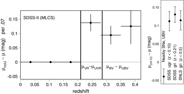
Figure 30. Left panel: redshift dependence of the average difference in μ for SDSS-II SNe between the nominal mlcs2k2 fits and fits in which the observer-frame passband corresponding to the rest-frame U band is excluded (g band for z > 0.21). Labels on the plot indicate the corresponding rest-frame UBV (Bessell 1990) passbands. Error bars  reflect the statistical uncertainty on the mean μ-difference in each redshift bin. Right panel: shift in average distance modulus when the rest-frame U band is excluded from the mlcs2k2 fits, for the subsamples discussed in the text.
Download figure:
Standard image High-resolution imageWe further investigate the U-band anomaly by comparing the fitted distance moduli with and without rest-frame U for three subsamples: (i) observer-frame UBV versus BV for 17 Nearby SNe Ia; (ii) observer-frame ugr versus gr for nine low-redshift SDSS-II SNe for which the u-band signal to noise is sufficient (z < 0.1), and (iii) observer-frame gri versus ri for 13 SNLS SNe with 0.21 < z < 0.5 and that have at least one g-band measurement within ±10 days of maximum brightness. In each case, the subsamples are chosen such that the light curves pass the selection criteria of Section 4 and include three observer passbands, one of which maps onto rest-frame U band. The differences in distance modulus (ΔμnoU,) between the two- and three-band fits (without and with rest-frame U) are shown in the right panel of Figure 30. The SDSS-II and SNLS subsamples show a consistent shift of about 0.1 mag. For comparison, the right panel of Figure 30 also shows the average shift for the points in the left-panel test at z > 0.21, again showing consistency. By contrast, the Nearby subsample is consistent with no shift or a slightly negative shift. Since the mlcs2k2 model is trained on a superset of the Nearby SN Ia data, we would expect no significant shift for the Nearby subsample. The redshift range z < 0.1 in the left panel of Figure 30 is not the same as the SDSS-ugr (z < 0.1) test in the right panel: the former is based on observer-frame gri and does not map onto rest-frame U band, while the latter is based on ugr versus gr in order to test excluding rest-frame U band.
Since the U band is particularly sensitive to host-galaxy extinction, it is worth exploring whether this anomaly might be an artifact of the assumed extinction law. We have repeated the test above, replacing the CCM89 color law nominally used in mlcs2k2 with the empirically determined salt-ii color law, CL(λ), in Equation (6). The salt-ii color law results in a U-band extinction that is 0.07 mag larger than that from using CCM89 with RV = 2.18 and the mean extinction value, AV = 0.35. The differences in the extinction for the other passbands are much smaller: 0.014, 0, 0.007, −0.002 for B, V, R, I. Repeating the U-band exclusion tests with the salt-ii color law results in distance-modulus offsets for the subsamples in the right panel of Figure 30 that are ∼20% smaller than for the nominal test using the CCM89 color law.
Although excluding rest-frame U band reveals a problem, it does not definitively indicate that rest-frame U, as opposed to one of the other passbands, is the source of the problem. To study this in more detail, we carry out a similar test in which observations in passbands corresponding to rest-frame B band are excluded. For SDSS-II SNe with redshifts z < 0.21, this B-exclusion test corresponds to comparing distance moduli from observer-frame gri (rest-frame BVR) with those from just r and i (rest-frame VR). The difference in the average distance modulus, μVR − μBVR, is −0.01 ± 0.02 mag, consistent with no shift. This test suggests that rest-frame B is not the source of the anomaly and strengthens the circumstantial evidence that rest-frame U is the source of the anomaly.
To further diagnose the U-band anomaly, we compare the light-curve data and the mlcs2k2 model light-curve fits as a function of epoch for the different rest-frame passbands and the five different SN samples. Figure 5 shows the data-model residuals for the nominal fits. Figure 31 shows the residuals when the filter corresponding to rest-frame U band is excluded from the fit; to see the U-band residuals, we must use the nominal mlcs2k2 model parameters that include the U band in the training. When the U band is excluded for the Nearby SNe Ia, there is a negligible change in the U-band residuals; this is expected because mlcs2k2 is trained on the nearby data. For the SDSS-II, excluding U band from the fits results in a ∼0.05 mag shift in the U-band residuals near the time of peak brightness (Trest = 0). The ESSENCE survey used only two passbands, R and I, and only a few of their SNe Ia probe rest-frame U band, so we cannot use this sample to probe the problem. For the SNLS sample, the residuals have been plotted for those SNe Ia that have observer-frame g-band measurements mapping into rest-frame U band (most of the SNe with z < 0.48), i.e., the same subset used in Figure 30. When the rest-frame U band is excluded, the corresponding shift in the U-band residuals is consistent with the shift seen in the SDSS-II. We have also examined the higher-redshift SNLS subset for which the observer-frame r band maps onto the rest-frame U band; the results of those tests are consistent with the tests based on the g band, but with much larger uncertainties. Note that the SNLS subset with an excluded g band has a spectroscopic efficiency spec = 1 (see Section 6.2), while the SDSS-II spectroscopic efficiency is significantly smaller than 1. Although the corresponding mlcs2k2 priors are quite different, the U-band anomaly is consistent between them, indicating that it is not caused by errors in spec.

Figure 31. Data-model fractional residuals as a function of rest-frame epoch in five-day bins for mlcs2k2 light-curve fits. Same as Figure 5, except fits exclude observer-frame filter corresponding to rest-frame U band.
Download figure:
Standard image High-resolution imageSince the mlcs2k2 model is trained with the Nearby sample, the U-band anomaly in the other SN Ia samples results in significant systematic uncertainties that limit the precision of cosmological parameters obtained with the current implementation of the mlcs2k2 method. There are a number of possible causes for the U-band discrepancy: (1) the SN Ia U-band flux could be redshift dependent; (2) selection effects for the Nearby sample could result in a U-band flux distribution that is not representative of the true SN Ia population; (3) there is a problem with the mlcs2k2 model; (4) the observer-frame U-band flux for the Nearby sample is not properly translated into the Landolt system; (5) the SN SED in the UV region is not adequately constrained, leading to errors in the K-corrections.
The first possibility, a redshift-dependent flux in the U band, is unlikely, given our test based on the ugr passbands for nine SDSS-II SN Ia with 0.04 < z < 0.09 (the right panel in Figure 30). Although this redshift range is still slightly higher than that for the Nearby sample  , a very rapid redshift evolution of SN Ia properties would be needed to account for the discrepancy. The second possibility is motivated by the very low selection efficiency for the Nearby sample, as indicated by the data-simulation comparison of the redshift distribution in the upper-left panel of Figure 9. However, the Nearby sample shows good agreement with the other SN Ia samples in the B, V, R passbands, so one would have to postulate a selection effect that biases the U band more than the other bands. The third possibility, of a problem with the light-curve model, is difficult to exclude, but the residuals in the Nearby sample ("Nearby" column of the left panel of Figure 5) look reasonable; this rules out obvious problems, thus narrowing potential problems to the extrapolation to higher redshifts and to different passbands.
The fourth possibility seems at first sight unlikely, since calibration errors are typically quoted at the level of 0.01–0.02 mag, but it could be that these errors have been underestimated. A mis-calibration of more than 0.1 mag in the U band would be needed to account for the observed anomaly. JRK07 reported that the light-curve residuals are 40% larger in the U band than in the other bands, but that does not necessarily point to a calibration problem. The U-band residuals for the Nearby sample (upper-left panel in Figure 5) vary with epoch as the SN becomes redder, suggesting a problem with the definition of the U-band filter.
The last possibility, a difference in the UV region of the SN SED, has been suggested in previous works (Foley et al. 2008; Sullivan et al. 2009). Both mlcs2k2 and salt-ii models assign larger uncertainties in the UV region compared to the redder bands. Ellis et al. (2008) found that maximum-light SN Ia SEDs varied significantly more at wavelengths λ < 4000 Å than for redder wavelengths and concluded that the additional dispersion is not due to extinction from host-galaxy dust.
Since the U-band anomaly appears in multiple samples (SDSS-II and SNLS) as well as in multiple redshift ranges for the SDSS-II sample (z < 0.1 and z > 0.21 in the right panel of Figure 30) we believe that the problem lies within the Nearby SN sample, i.e., with observations in the observer-frame U band. The most likely source of the problem is either the training procedure or the translation into the Landolt system. We will address this issue in the future by retraining light-curve models with SDSS-II SNe; the modeling of the rest-frame U band will make use of u-band measurements at z < 0.1 and g-band measurements at z > 0.21.
10.1.4. Comparison with WV07 Result
The Nearby+ESSENCE+SNLS sample combination (f) corresponds to one of the combinations analyzed by the ESSENCE collaboration in WV07 (with the exceptions of a different minimum redshift cut and different light-curve selection criteria). To compare with those results, we repeat the sample (f) analysis using the same BAO prior as in WV07, i.e., without the CMB prior. We find w = −0.75 ± 0.11(stat), which differs from the WV07 value by 0.32, or about 3σstat. Since the two analyses are based on the same data, the statistical significance of the discrepancy is much larger than 3σstat. If we add the systematic uncertainties in quadrature (δwsyst = 0.18), which is clearly an overestimate, the discrepancy is still fairly significant (1.8σ). Both analyses are based on the mlcs2k2 method, but our changes in mlcs2k2 parameters and priors result in systematic differences that are explained below.
We run the mlcs2k2 fitter in the "WV07 mode" (Section 5.1), using the WV07 parameter choices and reproducing their result for w, and then make cumulative changes in the analysis that evolve it toward the parameter inputs and light-curve fitting code used in our fiducial analysis. The resulting shifts in w relative to the WV07 value are shown in Figure 32. The changes from WV07 that we implement sequentially are change the minimum redshift for the Nearby sample from 0.015 to 0.02 (z > 0.02); set off-diagonal model covariances to zero (off-diag); implement K-correction improvements in item 2 of Section 5.1 (Kcor); replace the Bessell filter shifts introduced by Astier et al. (2006) and adopted by WV07 to the color transformation method used in our analysis and simultaneously change the primary standard from Vega to BD+17 (Calibration); use mlcs2k2 model parameters M, p, q (Equation (1)) corresponding to RV = 2.18 (Section 7.2), but still use RV = 3.1 and WV07 priors in the light-curve fits; use RV = 2.18 with WV07 priors in the light-curve fits; use the AV prior and efficiency from this analysis and remove the WV07 requirement that each observation has S/N >5 (prior).

Figure 32. Changes in w between the WV07 analysis and the analysis presented here, for the Nearby+ESSENCE+SNLS sample combination. Changes are implemented sequentially from left to right, and the cumulative differences in w are shown. The changes are described in the text.
Download figure:
Standard image High-resolution imageThe largest source of change in w (∼0.25) results from our different assumptions about host-galaxy dust and the mlcs2k2 fitting prior. Our fitting prior is based on a measurement of RV and of the AV distribution using the SDSS dust sample (Section 7) along with a comprehensive model of survey efficiencies using Monte Carlo simulations. In contrast to our analysis, the fitting prior used in WV07 is based on the assumption that RV = 3.1, that the AV distribution is represented by the glos distribution, and that the spectroscopic targeting efficiency is unity.
10.2. Results with salt-ii
Using the salt-ii method (Section 8.2), we present cosmological results for the six sample combinations (a)–(f) of Table 4. Table 14 gives the spectroscopic redshift and derived salt-ii fit parameters for each SN that passes the selection cuts of Section 4. Recall that the fit parameters x1 and c are estimated from the light-curve fits for each object. For each sample combination, these fit parameters are used to estimate the cosmological parameters, the global parameters α and β in Equation (29) (see Tables 16 and 17), and the distance moduli, by minimizing the scatter in the Hubble diagram. Since the distance-modulus estimate for each SN depends upon the sample combination in which the SN is included, upon the cosmological model parameterization, and upon the BAO and CMB priors, we provide tables for each of the six sample combinations and for both the FwCDM and ΛCDM models. Although the cosmological parameters have been corrected for the selection bias using simulations (Table 5), the distance moduli in Table 14 do not include any bias corrections. The entries in this Table should therefore not be used to derive cosmological constraints.
Table 14. salt-ii Light-Curve Fit Parameters Including BAO+CMB Priors (Uncertainties in Parentheses)
| SNID | Redshifta | μ | c | x1 | MJDpeak |
|---|---|---|---|---|---|
| 762 | 0.1904(.0000) | 39.91(0.09) | −0.01(0.03) | 0.73(0.33) | 53625.2(0.4) |
| 1032 | 0.1291(.0000) | 38.75(0.17) | 0.14(0.06) | −3.09(0.39) | 53626.6(0.4) |
| 1112 | 0.2565(.0000) | 40.53(0.16) | 0.00(0.04) | −1.06(0.69) | 53630.2(0.7) |
| 1166 | 0.3813(.0000) | 41.23(0.25) | 0.03(0.07) | 1.10(1.12) | 53631.9(1.2) |
| 1241 | 0.0858(.0000) | 37.91(0.09) | 0.09(0.03) | −0.90(0.17) | 53635.3(0.2) |
Notes. The complete set of tables for each sample combination (a)–(f) is given in the online journal, and also at http://das.sdss.org/va/SNcosmology/sncosm09_fits.tar.gz. aSpectroscopic redshift in CMB frame.
Only a portion of this table is shown here to demonstrate its form and content. A machine-readable version of the full table is available.
Download table as: DataTypeset image
10.2.1. salt-ii Hubble Dispersion
In the salt-ii method, an intrinsic dispersion (σintμ) is added in quadrature to the distance-modulus uncertainty (Equation (27)) such that the resulting Hubble diagram χ2μ/Ndof is equal to 1. Using the FwCDM model parameterization and the BAO+CMB prior, Table 15 gives the σintμ values obtained from fitting each SN sample independently and setting χ2μ = Ndof. For the Nearby, SDSS-II, and ESSENCE samples, the salt-ii values are similar to those from mlcs2k2 in the fourth line of Table 11. For the SNLS sample, the salt-ii dispersion is significantly smaller than that from mlcs2k2, while for the HST sample the salt-ii dispersion is larger. The smaller dispersion for SNLS may derive in part from the fact that the salt-ii model was partially trained on SNLS data. For sample combinations (a)–(f), the σintμ values are in Tables 16 and 17.
Table 15. Intrinsic Dispersion (σintμ) Required for χ2μ = Ndof for Each SN Ia Sample Fit Separately with the salt-ii Method
| σintμ for Sample | |||||
|---|---|---|---|---|---|
| Nearby | SDSS-II | ESSENCE | SNLS | HST | |
| Independent fits | 0.15 | 0.08 | 0.17 | 0.11 | 0.23 |
Download table as: ASCIITypeset image
Table 16. For the FwCDM Model, Constraints on w and ΩM from salt-ii SN Distances Combined with SDSS LRG BAO and WMAP-5 CMB Results
| Parameter | Result for Sample | |||||
|---|---|---|---|---|---|---|
| (a) | (b) | (c) | (d) | (e) | (f) | |
| σintμ | 0.084 | 0.124 | 0.105 | 0.128 | 0.140 | 0.160 |
| rmsμ | 0.178 | 0.219 | 0.170 | 0.210 | 0.232 | 0.231 |
| w | −0.87 | −0.98 | −0.92 | −0.98 | −0.96 | −0.95 |
| σw(stat) | 0.12 | 0.08 | 0.11 | 0.07 | 0.06 | 0.08 |
| σw(syst) | +0.06−0.12 | 0.15 | +0.07−0.15 | 0.13 | 0.12 | 0.13 |
| σw(tot) | +0.14−0.17 | 0.17 | +0.13−0.18 | 0.15 | 0.14 | 0.15 |
| ΩM | 0.281 | 0.256 | 0.271 | 0.264 | 0.265 | 0.267 |
 (stat) (stat) |
0.030 | 0.019 | 0.025 | 0.017 | 0.016 | 0.019 |
 |
+0.015−0.025 | 0.033 | +0.015−0.029 | 0.028 | 0.025 | 0.027 |
 |
+0.034−0.039 | 0.038 | +0.029−0.038 | 0.033 | 0.030 | 0.033 |
| α | 0.127 | 0.123 | 0.113 | 0.107 | 0.124 | 0.106 |
| σα(stat) | 0.017 | 0.015 | 0.014 | 0.013 | 0.014 | 0.019 |
| σα(syst) | 0.020 | 0.021 | 0.016 | 0.020 | 0.023 | 0.023 |
| σα(tot) | 0.026 | 0.026 | 0.021 | 0.024 | 0.027 | 0.030 |
| β | 2.52 | 2.62 | 2.50 | 2.66 | 2.64 | 2.56 |
| σβ(stat) | 0.16 | 0.13 | 0.15 | 0.12 | 0.12 | 0.17 |
| σβ(syst) | 0.11 | 0.19 | 0.11 | 0.19 | 0.18 | 0.25 |
| σβ(tot) | 0.19 | 0.23 | 0.19 | 0.22 | 0.22 | 0.30 |
Notes. (a)SDSS-only (b)SDSS+ESSENCE+SNLS (c)Nearby+SDSS (d)Nearby+SDSS+ESSENCE+SNLS (e)Nearby+SDSS+ESSENCE+SNLS+HST (f)Nearby+ESSENCE+SNLS
Download table as: ASCIITypeset image
Table 17. For the ΛCDM Model, Constraints on ΩM and ΩΛ from salt-ii SN Distances Combined with BAO and CMB Results
| Parameter | Result for Sample | |||||
|---|---|---|---|---|---|---|
| (a) | (b) | (c) | (d) | (e) | (f) | |
| σintμ | 0.085 | 0.123 | 0.105 | 0.128 | 0.140 | 0.160 |
| rmsμ | 0.177 | 0.220 | 0.170 | 0.210 | 0.232 | 0.231 |
| ΩΛ | 0.734 | 0.735 | 0.734 | 0.734 | 0.727 | 0.734 |
 |
0.019 | 0.017 | 0.019 | 0.017 | 0.016 | 0.017 |
 |
0.019 | 0.026 | 0.018 | 0.020 | 0.019 | 0.018 |
 |
0.027 | 0.031 | 0.026 | 0.026 | 0.025 | 0.025 |
| ΩM | 0.275 | 0.274 | 0.275 | 0.275 | 0.279 | 0.275 |
 |
0.023 | 0.021 | 0.023 | 0.020 | 0.019 | 0.021 |
 |
0.014 | 0.021 | 0.013 | 0.020 | 0.017 | 0.016 |
 |
0.027 | 0.030 | 0.027 | 0.029 | 0.026 | 0.027 |
| α | 0.126 | 0.123 | 0.113 | 0.113 | 0.116 | 0.105 |
| σα(stat) | 0.017 | 0.015 | 0.014 | 0.013 | 0.014 | 0.019 |
| σα(syst) | 0.020 | 0.021 | 0.016 | 0.019 | 0.023 | 0.023 |
| σα(tot) | 0.027 | 0.026 | 0.022 | 0.023 | 0.027 | 0.030 |
| β | 2.58 | 2.64 | 2.50 | 2.57 | 2.65 | 2.46 |
| σβ(stat) | 0.15 | 0.12 | 0.15 | 0.12 | 0.12 | 0.17 |
| σβ(syst) | 0.13 | 0.18 | 0.09 | 0.17 | 0.18 | 0.19 |
| σβ(tot) | 0.20 | 0.22 | 0.17 | 0.20 | 0.22 | 0.25 |
Download table as: ASCIITypeset image
10.2.2. salt-ii Hubble Diagrams and Cosmological Parameters
Figure 33 shows the differences between the salt-ii-estimated SN distance moduli μi and those for an open CDM model with no dark energy (ΩM = 0.3, ΩDE = 0) as a function of redshift. Figure 34 shows the distribution of normalized residuals, (μi − μFwCDM)/σμ, where μFwCDM is the distance modulus from the best-fit FwCDM model for sample combination (e) and σμ is the total uncertainty defined in Equation (27). The bulk of the distribution of all 288 normalized residuals (the upper-left panel of Figure 34) is well fitted by a Gaussian with σ = 0.75; outliers increase the rms to 0.92. The rms for combination (e) is slightly smaller than 1 because covariances from the fit are not included in the calculation of σμ.

Figure 33. Hubble residuals for the salt-ii method: differences between measured SN distance moduli and those for an open CDM model (ΩM = 0.3, ΩDE = 0) vs. redshift for the six SN sample combinations. Large, square (pink) points show weighted averages in weighted redshift bins (see the caption to Figure 24). Solid curves show the difference between the best-fit FwCDM model distance modulus for that sample combination and that for the open model, normalized to have the same value of the Hubble parameter. The error bars on the data points correspond to the distance-modulus error σfitμ from the salt-ii light-curve fit (Equation (27)), i.e., they do not include the intrinsic scatter or the effects of redshift and peculiar velocity errors. The vertical bars show the values of the intrinsic uncertainty, σintμ, included in the cosmology fits so that the χ2 per degree of freedom is unity for each Hubble diagram.
Download figure:
Standard image High-resolution image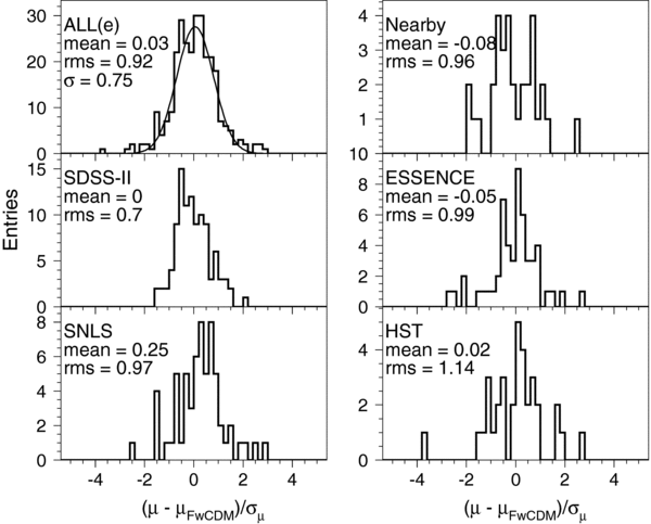
Figure 34. Distribution of normalized Hubble residuals (pull) for the salt-ii method, for sample combination (e) comprising all five samples (upper left, along with the Gaussian fit), and for each SN sample indicated on the panels. μ is the measured SN distance modulus, μFwCDM is the distance modulus from the best-fit FwCDM model for sample combination (e), and σμ is the total uncertainty (Equation (27)).
Download figure:
Standard image High-resolution imageFigures 35 and 36 show the salt-ii statistical-uncertainty contours for the FwCDM and ΛCDM models; for the latter, the salt-ii SN contours are more consistent with the BAO+CMB constraints than the mlcs2k2 contours were. For the combined SN+BAO+CMB results, the total uncertainty contours, including systematic errors, are shown in Figures 37 and 38. The best-fit cosmological parameter values and uncertainties, marginalizing over H0 and incorporating the bias corrections of Table 5, are given in Tables 16 and 17, respectively. The salt-ii statistical errors on cosmological parameters are consistent with those from mlcs2k2. The systematic errors for the two methods are similar for sample combinations (b) and (d)–(f), but the salt-ii systematic uncertainty is significantly smaller for the sample combinations in which SDSS-II is the high-redshift sample (a) and (c). The large difference in the systematic uncertainty is driven by the U-band anomaly.

Figure 35. For the FwCDM model, salt-ii statistical-uncertainty contours in the ΩM–w plane for each of the six SN sample combinations indicated on the plots. Long, black contours: 68%, 95%, and 99% confidence level regions for the SN data alone; green contours: corresponding CL regions for SDSS BAO (Eisenstein et al. 2005); blue contours: CL regions for WMAP-5 CMB (Komatsu et al. 2009); closed, black contours: combined constraints from SN+BAO+CMB.
Download figure:
Standard image High-resolution image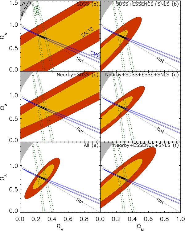
Figure 36. For the ΛCDM model, salt-ii statistical-uncertainty contours in the ΩM–ΩΛ plane for each of the six SN sample combinations indicated on the plots. Long, black contours: 68%, 95%, and 99% confidence level regions for the SN data alone; green contours: corresponding CL regions for SDSS BAO (Eisenstein et al. 2005); blue contours: CL regions for WMAP-5 CMB (Komatsu et al. 2009); closed, red contours: combined constraints from SN+BAO+CMB.
Download figure:
Standard image High-resolution image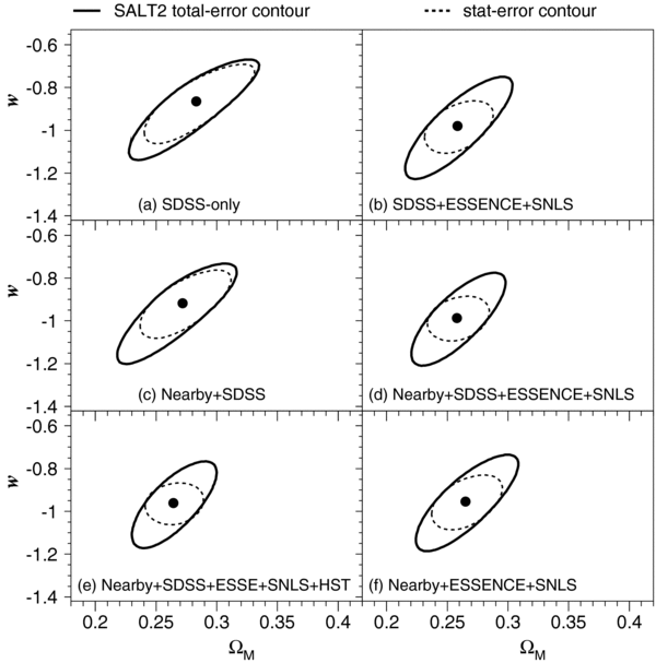
Figure 37. For salt-ii and the FwCDM model, 68% CL contours in the ΩM–w plane for each of the six SN sample combinations, using the combined SN+BAO+CMB constraints. Solid contours are total (statistical+systematic) uncertainty; dashed contours are statistical only. Systematic errors have been included using the prescription in Appendix F.
Download figure:
Standard image High-resolution image
Figure 38. For salt-ii and the ΛCDM model, 68% CL contours in the ΩM–ΩΛ plane for each of the six SN sample combinations, using the combined SN+BAO+CMB constraints. Solid contours are total (statistical+systematic) uncertainty; dashed contours are statistical only. Systematic errors have been included using the prescription in Appendix F.
Download figure:
Standard image High-resolution imageAmong the six SN sample combinations, the best-fit values of w for the FwCDM model again fall into two groups, as for the mlcs2k2 results, but with the opposite trend in w compared to mlcs2k2. For sample combinations (a) and (c), in which SDSS-II is the high-redshift sample, the salt-ii method results in w = −0.87 and −0.92, comparable to the mlcs2k2 results of −0.84 and −0.92 for the same sample combinations. However, for the other four sample combinations, which include higher-redshift SNe, salt-ii yields w = −0.98 to −0.95, compared with the mlcs2k2 result of w = −0.71 to −0.76 for the same sample combinations. Based on studies with simulated sample combinations, the observed difference between these two groups of salt-ii results is not statistically significant. However, the difference between the mlcs2k2 and salt-ii results for the higher-redshift samples appears to be significant. We discuss these differences further in Section 11.
10.2.3. Redshift Evolution of salt-ii Parameters
In the salt-ii model fits, α, β, and M (see Equation (29)) are global parameters that are assumed to be independent of redshift. To test the consistency of this assumption, we have carried out salt-ii fits separately in five redshift bins for sample combinations (d) and (e). For the fit in each redshift bin, the cosmological parameters w and ΩM in the FwCDM model are fixed to the values from the sample (e) fit, and the BAO+CMB prior is applied. The redshift dependence of the best-fit results for α, β, and M are shown in the left panels of Figure 39. There is evidence for redshift evolution of the parameters, particularly for the color parameter β, which falls with increasing redshift above z ∼ 0.6. This trend is more evident without the HST sample, suggesting that the β-variation is driven primarily by the SNLS sample. We have performed this test with high-statistics simulations (right panels of Figure 39) and find that the fitted salt-ii parameters are consistent across all redshift bins. Since the simulation accounts for the Malmquist bias, selection effects, and measurement errors, the redshift dependence favored by the data is likely due to some other effect.
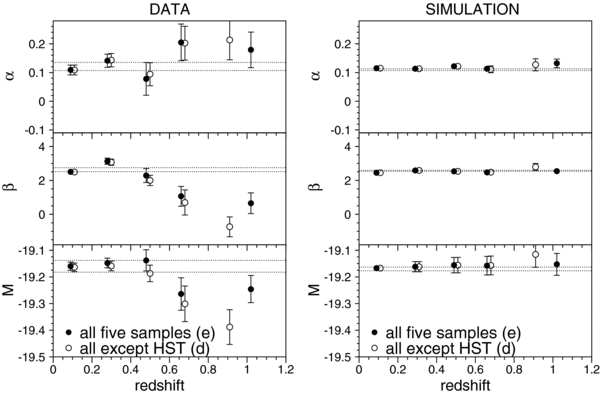
Figure 39. salt-ii fitted values and uncertainties for α, β, and M, evaluated independently in redshift bins for the Nearby+SDSS+ESSENCE+SNLS+HST sample combination (e) (solid dots) and for the Nearby+SDSS+ESSENCE+SNLS combination (d) (open circles). Left is for data; right is for a simulation with 10 times the number of SNe as in the data. For each redshift bin, the cosmological parameters w and ΩM are fixed to the values from the global combination ((d) or (e)) fit. The redshift bins are Δz = 0.2 for z < 0.8; the highest-redshift bin includes all SNe Ia with z > 0.8. The dashed lines show the ±1σ statistical error band based on the global fit to combination (e).
Download figure:
Standard image High-resolution image10.2.4. U-Band Anomaly with salt-ii
Here, we study how the U-band anomaly is manifest in the salt-ii method. Figure 40 shows the change in the binned SDSS-II SN Hubble diagram when the salt-ii fit excludes data from the observer-frame passband corresponding to the rest-frame U band, i.e., excluding g-band data for z > 0.21. Although this change only affects the light-curve fits for z > 0.21, it can alter the estimated distance moduli at all redshifts since they are derived from a global fit to the Hubble diagram. For z < 0.21, the average distance-modulus shift is (0.012 ± 0.003) mag; for z > 0.21, the mean shift is (0.079 ± 0.028) mag relative to the z < 0.21 shift. This relative shift is about half of that for mlcs2k2, but it is still significant: for the SDSS-only sample, the exclusion of the U band in the salt-ii fits results in a shift in w of −0.100 that is included as a systematic uncertainty.
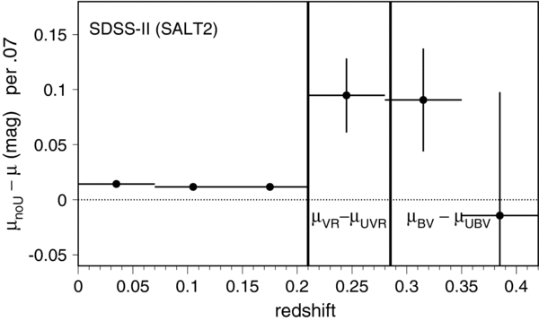
Figure 40. Redshift dependence of the average difference in distance modulus for SDSS-II SNe between the nominal salt-ii light-curve fits and fits in which the observer-frame passband corresponding to the rest-frame U band is excluded (g band for z > 0.21). Labels on the plot indicate the corresponding rest-frame UBVR (Bessell 1990) passbands. Error bars (rms/ ) reflect the statistical uncertainty on the mean μ-difference in each redshift bin.
Download figure:
Standard image High-resolution imageThe data-model residuals for the salt-ii light-curve fits are shown in Figure 7 for all of the SN Ia samples in all of the rest-frame passbands. Figure 41 shows the residuals when the filter corresponding to the rest-frame U band is excluded from the fit. In both cases, there are systematic discrepancies between the model and the data in the rest-frame U band for the Nearby SN Ia sample at all epochs. Since the salt-ii rest-frame U band model was trained primarily on higher-redshift SNe, i.e., downweighting observer-frame U-band data from Nearby SNe, this points to a systematic offset between the nearby, observer-frame U-band data and the higher-redshift, rest-frame U-band data, which was also qualitatively seen in the mlcs2k2 fits.

Figure 41. Data-model fractional residuals as a function of the rest-frame epoch in five-day bins for salt-ii light-curve fits. Same as Figure 7, except that fits exclude the observer-frame filter corresponding to the rest-frame U band.
Download figure:
Standard image High-resolution image11. COMPARISON BETWEEN mlcs2k2 AND salt-ii RESULTS
As noted in Section 10.2, the best-fit values of w for the FwCDM model agree between salt-ii and mlcs2k2 to within 0.04 for the SDSS-only and Nearby+SDSS sample combinations. However, as indicated in Tables 12 and 16, when the ESSENCE and SNLS data are included (sample combinations (b), (d), (e), and (f)), the w-values increase by ∼0.1 for the mlcs2k2 method, while decreasing by nearly 0.1 for the salt-ii method, leading to a discrepancy of Δw ∼ 0.2 between the two methods. To estimate the statistical significance of this discrepancy, we have run mlcs2k2 and salt-ii fits on a set of 10 simulated sample combinations generated with the mlcs2k2 model, each with the same statistics as the data. The predicted rms spread on Δw for combination (e) (all five samples) is Δwstat ≃ 0.05, so the observed discrepancy appears to be statistically significant.
To help diagnose this discrepancy, we compare the mlcs2k2 and salt-ii fitted parameters in Figure 42 for each of the SN samples. In this figure, the salt-ii parameters are based on the fit to sample combination (e), including the BAO+CMB prior, and the salt-ii distances have not been corrected for selection bias. The left panels show the mean difference in distance modulus, Δμ ≡ μSALT2 − μMLCS, as a function of redshift. The values of the Hubble parameter have been relatively adjusted so that the values of μ for the best-fit mlcs2k2 and salt-ii models for FwCDM agree at z → 0. The two methods yield consistent distance estimates for the Nearby, SDSS-II, and ESSENCE samples over the redshift ranges they cover. Moreover, the scatter in Δμ is comparable to the intrinsic scatter: σ(Δμ) = 0.10, 0.15, and 0.16 mag for these three samples, respectively. Analyzing the Nearby+SDSS+ESSENCE combination (not one of our standard combinations), w = −0.84 for mlcs2k2 and w = −0.89 for salt-ii, indicating good agreement. The situation changes dramatically when we include the SNLS data, for which there is a clear trend of increasing Δμ with redshift: this is the primary cause of the difference in w between mlcs2k2 and salt-ii for sample combinations (b), (d), (e), and (f).

Figure 42. Comparisons between mlcs2k2 and salt-ii light-curve fit parameters for the five SN samples: difference in distance modulus vs. redshift (left), color c vs. AV (middle), and x1 vs. Δ (right). Crosses in left panels show average and uncertainty in redshift bins. The solid straight lines (middle and right columns) are the same within a column to guide the eye, and they are derived from a fit to all of the samples except for ESSENCE, as explained in the text.
Download figure:
Standard image High-resolution imageThe middle and right panels of Figure 42 show the correlations between the mlcs2k2 and salt-ii light-curve fit parameters, salt-ii color c versus mlcs2k2 extinction AV and salt-ii versus mlcs2k2 shape-luminosity parameters x1 versus Δ. The fitted slopes, dc/dAV and dx1/dΔ, are consistent among the SN samples, except for ESSENCE which has somewhat larger slopes. The latter could be related to the fact that this sample has only two observer-frame passbands and hence less reliable color information.
The final light-curve fit parameter to compare is the epoch of maximum light in the rest-frame B band (t0). Figure 43 shows the distributions of t0(salt-ii)−t0(mlcs2k2) for the five SN samples. On average, the salt-ii epoch of peak light is about 1–1.5 days later than that for mlcs2k2, with a dispersion of about 1 day for the ground-based samples. For the HST sample, the offset is ∼2 days and the dispersion is larger (3 days) because of a handful of SNe with large t0-discrepancies. Fitting simulated SN samples shows that for the poorly sampled HST light curves, the fitted t0 from salt-ii is expected to be more discrepant from the input value than for mlcs2k2.
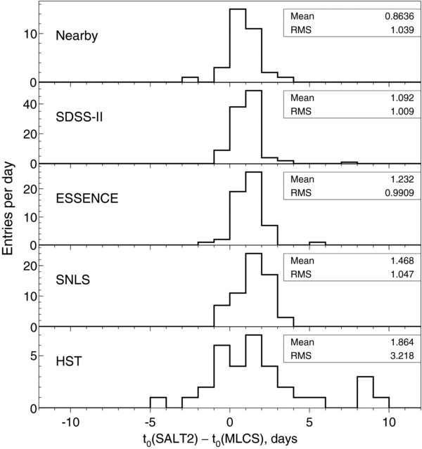
Figure 43. Comparison of salt-ii and mlcs2k2 fitted epoch of maximum B-band light for the five SN samples: shown are the distributions of t0(salt-ii)−t0(mlcs2k2). Insets show mean and rms for each sample.
Download figure:
Standard image High-resolution imageTo gain some insight into the discrepancy between the two fitting methods, we have investigated modifications to the mlcs2k2 model that are designed to partially replicate the features of the salt-ii model. The modifications are (1) change the mlcs2k2 model vectors so that the UBVRI light-curve templates match those of the synthesized salt-ii model, as described in Appendix G; (2) use a flat prior, Pprior(z, AV, Δ) = 1 in Equation (5), allowing negative values of AV; (3) use the salt-ii color law CL(λ) in place of the CCM89 model in the extinction term in Equation (1); and (4) exclude measurements for which the mean filter wavelength exceeds 7000 · (1 + z) Å. Using this modified mlcs2k2 model to fit the light curves, the resulting values of w decrease by 0.2 for sample combinations ((d) and (e)) and are in good agreement with the salt-ii results. Figure 44 compares the salt-ii parameters to those from the nominal mlcs2k2 fits and to those from the modified mlcs2k2 model. For the latter, the distance moduli show good agreement over the entire redshift range, and the correlations between the shape–color parameters (c versus AV and x1 versus Δ) are stronger than for the nominal mlcs2k2 fits.

Figure 44. For all five samples (combination (e)), comparison of salt-ii fit parameters with those from the nominal mlcs2k2 fits (left) and from the modified mlcs2k2 fits (right) as described in the text.
Download figure:
Standard image High-resolution imageOf the four modifications to mlcs2k2, the last two (use of the salt-ii color law and a 7000 Å cutoff) have a negligible effect on the cosmology analysis. The change in w is mainly due to matching the template light curves and to using a flat AV prior. Implementing either of these changes alone results in a w-shift of −0.07 or less; both changes are needed to obtain the full w-shift of −0.2. This exercise shows that the w-discrepancy between mlcs2k2 and salt-ii is related in part to the training procedure that determines the spectral and light-curve templates and in part to the different assumptions about SN color variations. The model V-band light curve and color evolution for mlcs2k2 and modified mlcs2k2 are compared in Figure 45 for different values of the shape-luminosity parameter Δ. The main discrepancy is in U − B, which differs by about 0.1–0.2 mag between mlcs2k2 and modified mlcs2k2. Since the modified mlcs2k2 colors agree well with the salt-ii colors (not shown), the U − B discrepancy in Figure 45 can be interpreted as the discrepancy between the mlcs2k2 and salt-ii models. In particular, since the models agree in the B band, this plot illustrates the differences in the rest-frame U band.
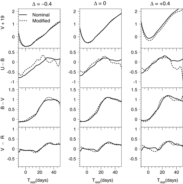
Figure 45. For the mlcs2k2 model, rest-frame V-band magnitude (top row) and colors (lower three rows) vs. epoch. Solid curves are for the nominal mlcs2k2 model and dashed curves are for the modified mlcs2k2 model. The latter was constructed to reproduce the salt-ii flux and color evolution. Each column corresponds to a different value of mlcs2k2 parameter Δ = −0.4, 0, 0.4. More than 70% of SNe Ia have Δ < 0 and 5% have Δ>0.4.
Download figure:
Standard image High-resolution imageAs noted earlier, there is strong evidence of systematic discrepancies in the rest-frame U band between the Nearby and higher-redshift samples. These discrepancies are reflected in the differences between the mlcs2k2 and salt-ii U-band models, differences that account for part of the cosmological parameter disagreement between the two models. The other major contributor to the cosmological disagreement is the differing treatment of SN color variation in the two models. There is a trend toward negative apparent salt-ii color at high redshift within the SNLS sample. salt-ii and mlcs2k2 with a flat-AV prior assign these blue events large intrinsic luminosities and therefore large distance moduli. By contrast, mlcs2k2 with the nominal AV prior identifies these events as having AV ∼ 0 and assigns them lower luminosities and distances. As illustrated in Figure 19, the nominal mlcs2k2 interpretation of these events is consistent with the observed color distributions, so it is not obvious which model is correct.
In Section 10, we have considered the approach of excluding data corresponding to the rest-frame U band altogether. In that case, for sample combinations that include ESSENCE and SNLS ((b), (d), (e), (f)), the salt-ii–mlcs2k2 discrepancy of Δw ∼ 0.2 is reduced by nearly 50%. By contrast, the same test applied to the SDSS-only sample increases Δw from 0.06 to 0.2 when the U band is excluded. Moreover, in the nominal fits (including the U band), the salt-ii and mlcs2k2 Hubble diagrams appear continuous around z = 0.2, and there is good agreement between them across the SDSS-II redshift range. Removing the U band introduces a noticeable step in both Hubble diagrams at z = 0.2, suggesting that both models display unphysical behavior when this information is removed completely. Such a sharp feature in the Hubble diagram is not well captured by a model with constant w, so the changes in Δw quoted above should be interpreted with extreme caution.
12. CONCLUSIONS
We have presented measurements of the Hubble diagram for type Ia SNe discovered during 2005 September–November by the SDSS-II SN Survey and combined them with other SN Ia data and with BAO and CMB results to derive cosmological constraints.
For the SDSS-II sample, based on stringent light-curve sampling and signal-to-noise criteria, we selected 103 SNe Ia with redshifts 0.04 < z < 0.42 for analysis from a parent sample of 130 spectroscopically confirmed SNe Ia. In an effort to make the analysis as homogeneous as possible among the SN data sets, we have used similar light-curve selection criteria and applied the same analysis techniques to all samples. We have estimated distances for these SNe using both the mlcs2k2 and salt-ii methods, which differ from each other in a number of respects (Section 5.3). The analysis includes significant improvements in the implementation of the mlcs2k2 method.
To determine the efficiency functions used in the mlcs2k2 priors and the biases in the salt-ii results, we have carried out detailed Monte Carlo simulations for each of the SN Ia data sets, making use of recorded observing conditions. The simulation accurately models the light curves (fluxes and errors) and the photometric selection effects; we have also incorporated a quantitative model for the spectroscopic selection efficiency based on comparing observed and simulated distributions in SN redshift and mean extinction. The simulation provides an excellent description of the data, as illustrated by the data-simulation comparison of the flux distribution for each SN sample (Figure 14).
Due to selection effects, SNe in spectroscopic samples tend to be brighter and less extinguished, on average, than those of the parent population. For SDSS-II, we have augmented the spectroscopic sample with a larger sample that includes photometrically identified SNe Ia with host-galaxy redshift measurements. We used this SDSS-II "dust" sample in conjunction with the Monte Carlo simulations to determine the mean host-galaxy reddening parameter RV and the distributions of extinction and light-curve shape parameters, P(AV) and P(Δ), for the underlying SN Ia population. By matching observed and predicted SN Ia colors in mlcs2k2, we find RV = 2.18 ± 0.14stat ± 0.48syst, consistent with the recent trend toward values lower than the canonical Milky Way average of 3.1. For comparison, the salt-ii analysis of the combined SN Ia sample (e) yields β = 2.64 ± 0.12(stat) ± 0.18(syst). If all SN Ia color variation (beyond that associated with the light-curve shape) were due to dust extinction, we would expect β − RV = 1. In this analysis we find β − RV = 0.5 ± 0.5, consistent with the expectation for extinction from dust, but also suggesting that there may be additional sources of SN color variation. We find that the underlying AV distribution is well described by an exponential function; this distribution is marginally consistent with both the galactic line of sight model used by WV07 and the exponential distribution found for the Nearby sample by JRK07.
For both the mlcs2k2 and salt-ii methods, we have carried out extensive studies of systematic errors, varying a large number of model parameters and assumptions, and we have included the resulting cosmological parameter variations in the systematic-error budget. For each method, the largest source of systematic uncertainty is associated with the rest-frame U-band anomaly. The anomaly is manifest in discrepancies between the light-curve data and the models, indicating the need for improved training of the rest-frame U-band models. When data corresponding to the rest-frame U band are excluded from the light-curve fits, the estimated distance modulus shifts by 0.12 mag for mlcs2k2 and by 0.08 mag for salt-ii. This shift occurs in particular redshift ranges, leading to abrupt features in the Hubble diagram; the effect is most severe for the SDSS-II SNe, since the U-band shift occurs at the median redshift of the sample. For this reason, and because dropping the U band leads to larger uncertainties from the significantly reduced color constraints, we have chosen not to exclude the U band for our nominal analysis but to include the corresponding changes as part of the systematic uncertainty.
We have combined the SN Hubble diagram with BAO and CMB measurements to estimate the cosmological parameters. For the FwCDM model and the combined sample of 288 SNe Ia from all five surveys, we find w = −0.76 ± 0.07(stat) ± 0.11(syst), ΩM = 0.307 ± 0.019(stat) ± 0.023(syst) using mlcs2k2 and w = −0.96 ± 0.06(stat) ± 0.12(syst), ΩM = 0.265 ± 0.016(stat) ± 0.025(syst) for salt-ii. This discrepancy of 0.2 in w between the two analysis methods is not due to inclusion of the SDSS-II data: for the Nearby+ESSENCE+SNLS (f) sample combination, which excludes SDSS-II, we find the same difference in w between the two methods. Our mlcs2k2 results for this sample combination (f) differ substantially from those of WV07 (Section 10.1.4), who used an earlier version of mlcs2k2 to analyze a nearly identical sample. We have traced the differences primarily to the different priors used, i.e., to the different values of RV, to the different AV distributions, and to the inclusion of spectroscopic targeting efficiency in the prior.
We have traced the mlcs2k2 versus salt-ii discrepancy to the SN model parameters determined in the training, particularly the rest-frame U-band model (Figure 45), and to the different assumptions about the source of color variations in mlcs2k2 and salt-ii. If we restrict the analysis to the 136 SNe Ia in the Nearby+SDSS combination, we find much better agreement between the two analysis methods, but with larger uncertainties, w = −0.92 ± 0.13(stat)+0.10−0.33(syst) for mlcs2k2 and w = −0.92 ± 0.11(stat)+0.07−0.15(syst) for salt-ii. We also note that the cosmological parameter uncertainties for the SDSS+ESSENCE+SNLS sample combination are similar to those for Nearby+ESSENCE+SNLS, i.e., the first-season SDSS-II data sample anchors the Hubble diagram with comparable power to the Nearby sample.
The mlcs2k2 versus salt-ii discrepancy for the higher-redshift samples raises the question of which method, if either, is more reliable. Since the mlcs2k2 U-band model relies entirely on U-band measurements at low redshift, while salt-ii uses a combination of low and high-redshift data, some at redder observer-frame passbands than U, the salt-ii results may be less biased by the U-band anomaly if the problem is related to the observer-frame U-band measurements. On the other hand, the salt-ii β parameter has a notable redshift dependence (Figure 39) that is inconsistent with the underlying assumption that it is constant. Concerning the interpretation of SN color variations, both models are consistent with the data; in particular, an SN that is bluer than the templates could be extremely bright, as indicated by salt-ii, or it could be due to measurement uncertainty and intrinsic color fluctuations, as interpreted by mlcs2k2 (Figure 19). Since we cannot definitively determine from the current data that either method is better or incorrect, the overall conclusion is that the cosmological parameter w conservatively lies between −1.1 and −0.7. This result reflects the fact that present SN Ia samples have reached the systematic limits of current SN model fitters. Although this result is disappointing, we are optimistic that this situation is temporary. The full three-season SDSS-II sample, with its homogeneous and well-modeled selection function, will serve both to anchor the Hubble diagram and to retrain the light-curve models. Since the U-band anomaly is most likely associated with the published Nearby SN sample, use of the full SDSS-II data as well as updated low-redshift samples from the CfA (Hicken et al. 2009a), the Carnegie Supernova Project, and the Nearby Supernova Factory should significantly reduce this major source of systematic uncertainty.
Finally, our use of photometrically identified SNe Ia to measure host-galaxy dust properties is an important step toward including these SNe in the Hubble diagram, which will increase the statistical power of the data. This will be a growing trend in the future, as large surveys, including PanSTARRS, the Dark Energy Survey, and LSST, will discover vastly more SNe than can be confirmed with available spectroscopic resources.
All software used in this analysis is publicly available from our Web site (Kessler et al. 2009). We wish to thank J. Guy for retraining the salt-ii program and for consulting on its use and results. We thank Armin Rest for modifying the ESSENCE SN-search pipeline for use in the SDSS SN survey. We gratefully acknowledge support from the Kavli Institute for Cosmological Physics at the University of Chicago, the National Science Foundation at Wayne State, the Japan Society for the Promotion of Science (JSPS), and the Department of Energy at Fermilab, the University of Chicago, and Rutgers University. R.J.F. is supported by a Clay Fellowship. Y. Ihara and T. Morokuma are supported by a JSPS Fellowship. A.V.F. is grateful for the support of NSF grant AST-0607485 and DOE grant DE-FG02-08ER41563. Funding for the creation and distribution of the SDSS and SDSS-II has been provided by the Alfred P. Sloan Foundation, the Participating Institutions, the National Science Foundation, the U.S. Department of Energy, the National Aeronautics and Space Administration, the Japanese Monbukagakusho, the Max Planck Society, and the Higher Education Funding Council for England. The SDSS Web site is http://www.sdss.org/.
The SDSS is managed by the Astrophysical Research Consortium for the Participating Institutions. The Participating Institutions are the American Museum of Natural History, Astrophysical Institute Potsdam, University of Basel, Cambridge University, Case Western Reserve University, University of Chicago, Drexel University, Fermilab, the Institute for Advanced Study, the Japan Participation Group, Johns Hopkins University, the Joint Institute for Nuclear Astrophysics, the Kavli Institute for Particle Astrophysics and Cosmology, the Korean Scientist Group, the Chinese Academy of Sciences (LAMOST), Los Alamos National Laboratory, the Max-Planck-Institute for Astronomy (MPA), the Max-Planck-Institute for Astrophysics (MPiA), New Mexico State University, Ohio State University, University of Pittsburgh, University of Portsmouth, Princeton University, the United States Naval Observatory, and the University of Washington.
This work is based in part on observations made at the following telescopes. The Hobby-Eberly Telescope (HET) is a joint project of the University of Texas at Austin, the Pennsylvania State University, Stanford University, Ludwig-Maximillians-Universität München, and Georg-August-Universität Göttingen. The HET is named in honor of its principal benefactors, William P. Hobby and Robert E. Eberly. The Marcario Low-Resolution Spectrograph is named for Mike Marcario of High Lonesome Optics, who fabricated several optical elements for the instrument but died before its completion; it is a joint project of the Hobby-Eberly Telescope partnership and the Instituto de Astronomía de la Universidad Nacional Autónoma de México. The Apache Point Observatory 3.5 m telescope is owned and operated by the Astrophysical Research Consortium. We thank the observatory director, Suzanne Hawley, and site manager, Bruce Gillespie, for their support of this project. The Subaru Telescope is operated by the National Astronomical Observatory of Japan. The William Herschel Telescope is operated by the Isaac Newton Group on the island of La Palma in the Spanish Observatorio del Roque de los Muchachos of the Instituto de Astrofisica de Canarias. The W. M. Keck Observatory is operated as a scientific partnership among the California Institute of Technology, the University of California, and the National Aeronautics and Space Administration. The Observatory was made possible by the generous financial support of the W. M. Keck Foundation.
APPENDIX A: SPECTRAL WARPING FOR K-CORRECTIONS IN THE mlcs2k2 LIGHT-CURVE MODEL
The mlcs2k2 model makes predictions about rest-frame light curves in UBRVI; K-corrections are used to translate the model light curves so that they can be used to fit measurements at non-zero redshift in a variety of passbands. This translation requires knowledge of the SN SED time sequence. Since the SN Ia population exhibits intrinsic color variations, a single time sequence will not provide an adequate model. The standard practice is therefore to "warp" the model SEDs so that they match the colors of the photometric model for a given object. Here we describe our procedure for the spectral warping used in determining K-corrections within the mlcs2k2 framework (Section 5.1).
The procedure begins by computing the rest-frame mlcs2k2 model magnitudes for the assumed values of extinction (AV), time of peak brightness (t0), and shape-luminosity parameter (Δ). These assumed values are typically determined iteratively as part of the χ2-minimization (Equation (3)). For each iteration, an epoch-dependent SN Ia SED from Hsiao et al. (2007) is warped so that the synthetic colors of the warped SED match the mlcs2k2 model colors at the corresponding rest-frame epoch.
In detail, for each epoch and passband, the rest-frame model magnitude is first computed as the sum of the first four terms on the right-hand side of Equation (1), where the host-galaxy extinction Xhost has been determined from the unwarped SED using the values of AV and RV. Although the K-correction depends strongly on how the SED is warped, the value of Xhost is only weakly dependent on the warping, so Xhost can be determined to good approximation from the unwarped SED. As an illustration, when the SED is severely warped to modify the V − B color (at peak brightness) by 0.5 mag, the estimate of the V-band extinction changes by less than 1%. Next, the SED is warped by multiplying it with the CCM89 galactic extinction law, following JRK07. This usage of the CCM89 law to warp is purely a mathematical convenience—it has nothing to do with physical extinction. The "AV-warp" is the value of "AV" in the warp factor for which the synthetic SN Ia color matches the color of the rest-frame model magnitude computed above. The redshift-dependent K-correction to the observer-frame magnitude is then determined from this AV-warped SED, using the redshift and knowledge of the rest-frame and observer-frame passbands. This method is model independent and can therefore be applied to any light-curve model. The SED is warped independently at each epoch and locally in wavelength near the passband of interest; we do not do a global fit to match all colors simultaneously. There are two potential limitations in this procedure. First, brightness-dependent spectral features are ignored, i.e., we use a single, Δ-independent composite SED at each epoch. Second, for the rest-frame U band (I band) there is no constraint for warping the SED blueward (redward) of the central wavelength.
Compared to the treatment in JRK07, we have made a slight improvement to the spectral warping used for K-corrections. The rest-frame filter, f', is chosen as the one that covers the equivalent rest-frame wavelength, λrest = λobs/(1 + z), where λobs is the central wavelength of the observed passband f. For spectral warping, JRK07 used a fixed rest-frame color for a given rest-frame filter, e.g., B − V color was used when f' = B. In this example, the new code uses either B − V or B − U for the warping, depending on whether the value of λrest is closer to the central wavelength of V or U.
APPENDIX B: FILTER SET FOR THE NEARBY SN IA SAMPLE
The Nearby SN Ia sample serves as the low-redshift anchor for the Hubble diagram. A superset of the Nearby sample was also used to derive ("train") model parameters for the mlcs2k2 method. Within the framework of mlcs2k2, here we discuss the filter-response functions and color terms needed for the K-corrections that transform from rest-frame model magnitudes (UBVRI) to observer-frame magnitudes.
The Nearby SN Ia sample is a heterogeneous data set for which the filter response functions vary. While some of the filter curves have been published, the applicability of the filter curves to precision photometry is uncertain. However, all of the Nearby SN Ia magnitudes have been transformed into the Landolt system (Landolt & Umoto 2007), even if the color terms are not always available. Although the Landolt magnitude system is well defined, there are no standard filter responses for this system and hence one cannot compute K-corrections. In order to compute K-corrections, we determine color transformations from the Landolt system to the standard UBVRI filter response functions defined by Bessell (1990). While previous analyses with SNe Ia used Vega as the primary reference, we note that Vega has not been measured by Landolt. Instead of using Vega, we define the primary reference from the Landolt network, BD+17°4708 (hereafter BD+17), which happens to be the primary reference for SDSS photometry and also has a precisely measured HST spectrum.
In order to determine the Bessell–Landolt transformation, we use Landolt standards that have excellent spectrophotometric data and compare the observed Landolt magnitudes to synthetic Bessell magnitudes based upon the spectrophotometric data and knowledge of the Bessell response functions. We use spectra from HST CALSPEC 200646 (Bohlin 2007) because of its availability, high quality, and consistent calibration. For the Landolt standards that overlap with HST CALSPEC, the Landolt measurements are given in Table 18 and the synthetic magnitudes in the Bessell system in Table 19.
Table 18. Measurements from Landolt 2007 that Overlap with HST CALSPEC Data
| Star | Nobs | V | B − V | U − B | V − R | R − I | V − I |
|---|---|---|---|---|---|---|---|
| BD+17°4708a | 28 | 9.464 | 0.443 | −0.183 | 0.298 | 0.320 | 0.618 |
| ... | ... | ±0.0026 | ±0.0015 | ±0.0021 | ±0.0011 | ±0.0009 | ±0.0013 |
| Vegab | ... | 0.017 | −0.002 | −0.004 | −0.007 | 0.004 | −0.003 |
| ... | ... | x | x | x | x | x | x |
| G191B2Bc | 48 | 11.773 | −0.326 | −1.205 | −0.149 | −0.181 | −0.327 |
| ... | ... | ±0.0028 | ±0.0014 | ±0.0026 | ±0.0016 | ±0.0017 | ±0.0025 |
| GD71d | 104 | 13.032 | −0.249 | −1.107 | −0.137 | −0.164 | −0.320 |
| ... | ... | ±0.0015 | ±0.0014 | ±0.0024 | ±0.0015 | ±0.0022 | ±0.0028 |
| GD153e | 4 | 13.346 | −0.286 | −1.169 | −0.138 | −0.180 | −0.319 |
| ... | ... | ±0.004 | ±0.004 | ±0.005 | ±0.006 | ±0.008 | ±0.002 |
| AGK+81°4211a | 39 | 11.936 | −0.340 | −1.204 | −0.154 | −0.191 | −0.345 |
| ... | ... | ±0.0024 | ±0.0013 | ±0.0030 | ±0.0013 | ±0.0021 | ±0.0019 |
| BD+28°4211a | 32 | 10.509 | −0.341 | −1.246 | −0.147 | −0.176 | −0.322 |
| ... | ... | ±0.0027 | ±0.0018 | ±0.0039 | ±0.0011 | ±0.0012 | ±0.0018 |
| BD+75°325a | 37 | 9.548 | −0.334 | −1.212 | −0.150 | −0.187 | −0.336 |
| ... | ... | ±0.0018 | ±0.0010 | ±0.0020 | ±0.0008 | ±0.0018 | ±0.0018 |
| Feige 110 e | 26 | 11.832 | −0.305 | −1.167 | −0.138 | −0.180 | −0.313 |
| ... | ... | ±0.0018 | ±0.0010 | ±0.0033 | ±0.0012 | ±0.0022 | ±0.0020 |
| Feige 34a | 31 | 11.181 | −0.343 | −1.225 | −0.138 | −0.144 | −0.283 |
| ... | ... | ±0.0025 | ±0.0011 | ±0.0041 | ±0.0013 | ±0.0018 | ±0.0018 |
| GRW+70°325a | 36 | 12.773 | −0.091 | −0.875 | −0.100 | −0.104 | −0.206 |
| ... | ... | ±0.0027 | ±0.0017 | ±0.0022 | ±0.0013 | ±0.0017 | ±0.0020 |
| HZ21a | 40 | 14.688 | −0.327 | −1.236 | −0.149 | −0.201 | −0.350 |
| ... | ... | ±0.0022 | ±0.0016 | ±0.0033 | ±0.0022 | ±0.0043 | ±0.0049 |
| HZ44a | 40 | 11.673 | −0.291 | −1.196 | −0.141 | −0.181 | −0.322 |
| ... | ... | ±0.0016 | ±0.0011 | ±0.0027 | ±0.0009 | ±0.0011 | ±0.0014 |
| HZ4a | 51 | 14.506 | 0.086 | −0.675 | −0.074 | −0.060 | −0.136 |
| ... | ... | ±0.0027 | ±0.0017 | ±0.0022 | ±0.0013 | ±0.0017 | ±0.0020 |
Notes. Nobs is the number of Landolt observations. aVega measurements are not from Landolt. The V mag is from the HST analysis of Bohlin (2007) and the colors are from Bessell et al. (1998). Vega error estimates are not given in the references. bThe reported V magnitude was adjusted by Bohlin (2000). The magnitude reported by Landolt (2007) is 11.781. The errors and the colors are from Landolt loc cit. cA. Landolt 2006, private communication. dA. Landolt (2006, private communication) reported more observations but the same values as published previously (Landolt 1992). eLandolt (2007).
Download table as: ASCIITypeset image
Table 19. For Landolt Stars in Table 18, Synthetic Magnitudes are Computed Using HST CALSPEC Spectra and Filters Defined by Bessell (1990)
| Star | V | B − V | U − B | V − R | R − I |
|---|---|---|---|---|---|
| BD+17°4708 | 9.4640 | 0.4430 | −0.1830 | 0.2980 | 0.3200 |
| Vega | 0.0169 | 0.0048 | 0.0213 | −0.0114 | −0.0086 |
| G191B2B | 11.7777 | −0.3021 | −1.2475 | −0.1535 | −0.2016 |
| GD71 | 13.0371 | −0.2265 | −1.1476 | −0.1438 | −0.1840 |
| GD153 | 13.3509 | −0.2583 | −1.1933 | −0.1477 | −0.1916 |
| AGK+81°4211 | 11.9226 | −0.3221 | −1.2573 | −0.1583 | −0.2051 |
| BD+28°4211 | 10.5076 | −0.3202 | −1.2735 | −0.1581 | −0.2122 |
| BD+75°325 | 9.5301 | −0.3136 | −1.2672 | −0.1509 | 0.1987 |
| Feige 110 | 11.8295 | −0.2969 | −1.2064 | −0.1475 | −0.1697 |
| Feige 34 | 11.1731 | −0.3312 | −1.2726 | −0.1334 | −0.1563 |
| GRW+70°5824 | 12.7515 | −0.0605 | −0.8913 | −0.1118 | −0.1287 |
| HZ21 | 14.6880 | −0.3270 | −1.2677 | −0.1346 | −0.1969 |
| HZ44 | 11.6606 | −0.2643 | −1.2213 | −0.1385 | −0.2001 |
| HZ4 | 14.4818 | 0.1210 | −0.6627 | −0.0879 | −0.0758 |
Download table as: ASCIITypeset image
To proceed, we define a synthetic Landolt magnitude in passband "X" by

where XBesssynth is the synthetic magnitude constructed from the source spectrum and the filter response from Bessell (1990) and ΔXsynth is a correction based on color transformations as follows:
The subscript "obs" refers to observed (instrumental) magnitudes for a standard star or SN and the BD+17 subscript indicates a Landolt measurement. These color transformations are defined so that there is no correction for the reference star, BD+17. The color coefficients (ki = 0,4) are determined by fitting Equation (B2) with the Landolt measurements and synthetic Bessell magnitudes in Tables 18 and 19, with Vega excluded from the fit. The resulting ki values are shown in Table 20; typical values are in the few percent range. We have also calculated the color terms determined with Vega as the primary reference, with results given in the last column of Table 20. The use of color terms is an approximation that can lead to significant errors, but the small size of the color terms indicate that this error should be negligible.
Table 20. Calculated Color Coefficients for BD+17 and for Vega
| Band | Coefficient | Value for BD+17°4708 | Value for Vega |
|---|---|---|---|
| V | k0 | −0.010 ± 0.004 | −0.015 ± 0.004 |
| B − V | k1 | +0.027 ± 0.005 | +0.033 ± 0.005 |
| U − B | k2 | −0.035 ± 0.004 | −0.050 ± 0.004 |
| V − R | k3 | −0.010 ± 0.005 | +0.004 ± 0.005 |
| R − I | k4 | −0.029 ± 0.007 | −0.010 ± 0.007 |
Download table as: ASCIITypeset image
As an alternative to using color transformations, we follow Astier et al. (2006) and define a modified set of UBVRI Bessell filter response functions in which the central wavelength of each filter passband is shifted from that of Bessell (1990) but the shape of the response curve is unchanged. The shifts are defined such that the color terms, as defined in Equation (B2), are zero. The corresponding wavelength shifts relative to the filter responses defined by Bessell (1990) are given in Table 21 under the column "HST standards." The shifts used in Astier et al. (2006) are also given in Table 21 for comparison. The differences in wavelength shifts are likely due to the different choices of spectral standards: we use HST standards (Table 18), while Astier et al. (2006) used ground-based spectra from Hamuy et al. (1992, 1994).
The recipe for K-corrections is as follows. The UBVRI model magnitudes for mlcs2k2 are assumed to be in the Landolt system. The inverse of Equation (B2) is used to convert these Landolt magnitudes into magnitudes in the Bessell (1990) system, and then a K-correction is applied in the usual manner. For the SDSS, ESSENCE, and SNLS surveys, the filter response functions are well understood, and therefore the K-corrections are well defined. For the Nearby SN sample, the K-correction transforms into a hypothetical observer-frame UBVRI system with a filter response described by Bessell (1990); in this case, Equation (B2) is again applied to transform back to Landolt magnitudes.
APPENDIX C: PRIMARY MAGNITUDES FOR BD+17 AND VEGA
For the mlcs2k2 method, the primary magnitudes for each filter system are given in Table 22 for BD+17 and Vega. The magnitudes for UBVRI are taken from Landolt measurements and the SDSS gri magnitudes are given in the AB system. The primary magnitudes in the other filter systems are obtained by the interpolation method described below.
Table 21. Wavelength Shifts for the Bessell (1990) Filters
| Filter Shift in Å for: | ||
|---|---|---|
| Bessell filter | HST standards | Astier et al. (2006) |
| U | +13 ± 4 | ... |
| B | −15 ± 4 | −41 |
| V | +12 ± 6 | −27 |
| R | +7 ± 9 | −21 |
| I | −45 ± 21 | −25 |
Download table as: ASCIITypeset image
Table 22. Primary Landolt Magnitudes Used for K-corrections
| Filter System | Primary | Magnitudes |
|---|---|---|
| Landolt U, B, V, R, Ia | BD+17 | 9.724, 9.907, 9.464, 9.166, 8.846 |
| Vega | 0.017, 0.021, 0.023, 0.030, 0.026 | |
| SDSS 2.5 m g, r, i | BD+17 | 9.644, 9.350, 9.256 |
| (AB system) | Vega | −0.106, 0.142, 0.356 |
| CTIO(ESSENCE) R, Ib | BD+17 | 9.152, 8.855 |
| Vega | 0.024, 0.020 | |
| CFHT(SNLS) g, r, i, zb | BD+17 | 9.720, 9.222, 8.911, 8.756 |
| Vega | 0.016, 0.022, 0.021, 0.016 | |
| HST (F110W, F160W, | BD+17 | 8.558, 8.141, 9.337, 8.898, 8.746 |
| F606W, F775W, F850LP)b | Vega | 0.003, 0.000, 0.020, 0.021, 0.015 |
Notes. aMeasured by Landolt. bInterpolated as described in the text.
Download table as: ASCIITypeset image
We compute the BD+17 magnitudes by first interpolating UBVRI magnitudes from Vega and using these magnitudes to determine offsets that are used to correct the synthetic magnitudes (from HST spectra) for BD+17. The Vega interpolation is based solely on the central wavelength of each passband and does not depend on the detailed shape of the transmission curve. This approach is reasonable since the Vega magnitudes and colors are all small, and the Vega spectrum is smooth.
Since we use the published magnitudes for the SN data, using our own analysis of the BD+17 magnitudes means that we have effectively adjusted the photometry of the published data. The implicit assumption is that the original photometry is correct relative to Vega, but that Vega itself has a slightly different value than was assumed previously. The Vega and BD+17 magnitudes do not agree exactly with the difference expected for the synthetic magnitudes computed from the HST spectra, so Vega and BD+17 define slightly different photometric systems. While we believe that our use of BD+17 provides an accurate and more consistent description of all the photometric data, it should be emphasized that our assumed magnitudes for Vega differ by amounts that are small compared to the zero-point errors quoted in the original publications and the differences are well within our quoted systematic errors.
As an example, we illustrate the determination of the primary BD+17 magnitudes for the SNLS griz passbands. For the interpolation, we need Landolt UBVRI magnitudes referenced to BD+17, MLandVega = MsynthVega + (MLandBD17 − MsynthBD17). For the V band, MLandVega(V) = 0.003 + (9.464 − 9.450) = 0.017 mag. The results for all passbands are  , 0.022, 0.017, 0.028, 0.037 mag. We interpolate these UBVRI magnitudes to the central wavelengths of the SNLS griz filters to get interpolated Vega magnitudes (MinterpVega), with the results shown in the first row of Table 23. The zero-point offsets for synthetic magnitudes (ZPsynth) are the differences between the interpolated and synthetic magnitudes for Vega. The BD+17 magnitudes in the Landolt system are then given by MLandBD17 = MsynthBD17 + ZPsynth, and the results are given in the seventh row of Table 22.
Table 23. Magnitudes Used to Compute Landolt BD+17 Magnitudes for SNLS griz
| Type of Magnitude | Magnitude | |||
|---|---|---|---|---|
| g | r | i | z | |
| MinterpVega | 0.020 | 0.025 | 0.035 | 0.030 |
| MsynthVega | −0.099 | 0.149 | 0.376 | 0.513 |
| ZPsynth | 0.119 | −0.124 | −0.341 | −0.483 |
| MsynthBD17 | 9.601 | 9.346 | 9.253 | 9.240 |
Download table as: ASCIITypeset image
APPENDIX D: DETERMINING THE UNDERLYING DISTRIBUTION OF EXTINCTION (AV) AND LIGHT-CURVE SHAPE (Δ)
Within the framework of the mlcs2k2 model (Section 5.1), we extract the underlying AV and Δ distributions from the SDSS dust sample (Section 7.1) by making use of simulated light curves processed in exactly the same way as the observed light curves. The underlying distributions of AV and Δ are defined such that when these underlying distributions are input into the simulation, the fitted distributions from the simulated light curves match the data distributions. We assume that these underlying distributions are independent of redshift, and we fix the CCM89 extinction law parameter to RV = 2.18, following the analysis of Section 7.2.
Here we use the Bayesian unfolding method of D'Agostini (1995), and tests with simulated samples show that one iteration is adequate with our statistics. For this discussion, we use an asterisk superscript to indicate the underlying true value for a parameter; the lack of an asterisk indicates a measured value obtained from fitting with the mlcs2k2 method. Simulated light curves are generated with a flat distribution in A*V (over the range 0–4), a flat distribution in Δ* (from −0.6 to +2), and a flat distribution in redshift (from 0 to 0.4). For each simulated light curve that passes the selection criteria of Section 4, the mlcs2k2 model is used with a flat, non-informative prior on AV and Δ to extract a fitted value of AV and Δ. These fitted values, in general, are different from the underlying A*V and Δ*. The accuracy of the inferred extinction, AV − A*V, has a typical rms of 0.2, with little dependence on redshift. The accuracy of the fitted shape-luminosity parameter, Δ − Δ*, has an rms of a few hundredths for z < 0.1, and the rms increases to about 0.2 at z ∼ 0.3.
We use the simulation to calculate the conditional probability of extracting fitted values of AV and Δ from a light curve generated with values A*V and Δ*, as a function of redshift. Since the generated, fitted, and observed values are drawn from continuous distributions, we bin these quantities with bin sizes of 0.2 for AV, 0.1 for Δ, and 0.05 for redshift. Each bin is identified by an index:  for generated quantities and
  for fitted quantities. Since redshifts are spectroscopically determined with high precision, we always have iz = i*z. From the simulation, we calculate the conditional probability distribution

where  is the number of fits producing values of (AV, Δ, z) that lie in the specified bins and
  is the number of light curves generated with (A*V, Δ*, z*) that lie in the specified bins. The underlying two-dimensional distribution of A*V and Δ* is then obtained from the SDSS-II data by
where sim = subtr × cuts is the simulated efficiency that includes the combined effects of the image-subtraction pipeline (Section 6.2) and selection cuts (Section 4),  is the number of observed SNe Ia in redshift bin iz with fitted AV, Δ that lie in the specified bins, and the summation is over the three-dimensional grid of observed AV, Δ, and redshift. The corresponding one-dimensional distributions, P(A*V) and P(Δ*), are obtained by marginalizing the two-dimensional distribution over the other variable. We have extensively tested this procedure for extracting the true distributions of A*V and Δ* on simulated data samples, and the technique gives excellent agreement between the true (generated) distributions and the distributions extracted from the simulated data.
We apply this technique to the SDSS-II dust sample; the extracted A*V and Δ* distributions are shown in Figure 46. The error bars reflect the statistics of our data sample as well as the statistical uncertainties in the simulated efficiency and Psim distributions. We fit these distributions to analytic functions that can be easily computed for the mlcs2k2 fitting prior. The underlying A*V distribution is accurately fitted by an exponential function

The Δ* distribution is described by a bifurcated Gaussian with peak position Δ0 and different positive side and negative side widths, σ+ and σ −, respectively. We find


where the uncertainties are statistical and systematic, respectively. These distributions are the basis for the mlcs2k2 priors shown in Figure 17.

Figure 46. Distributions of A*V and Δ* based on the SDSS-II dust sample and the procedure described in the text. The A*V distribution includes overlays of the best-fit exponential function (solid curve) and the glos prior (dashed).
Download figure:
Standard image High-resolution image
In addition to the statistical errors, we have considered a number of systematic effects in the determination of these distributions. We vary RV by ±1σ (see Section 7.2); this variation has the largest effect on the inferred A*V distribution. We vary the maximum redshift for the SN Ia light curves included in the data sample from the nominal 0.30 to 0.25. We also consider the difference between the two different methods for modeling SN Ia intrinsic luminosity variations (see Section 6.1). Numerous minor variations in the analysis procedure, such as changing bin sizes and the use of binned or smoothed efficiencies, have a negligible effect. The uncertainties are summarized in Table 24 and are summed in quadrature to obtain the total uncertainty.
Table 24. Uncertainties in the Parameters that Describe the Distributions of A*V (τV) and Δ* (Δ0, σ +, σ−)
| Source of Uncertainty | Uncertainty | |||
|---|---|---|---|---|
| τV | Δ0 | σ+ | σ− | |
| Statistical | 0.050 | 0.054 | 0.051 | 0.033 |
| RV = 2.18 ± 0.50 | 0.050 | 0.005 | 0.004 | 0.008 |
| Redshift range | 0.040 | 0.012 | 0.014 | 0.004 |
| Simulated color smearing | 0.030 | 0.003 | 0.001 | 0.006 |
| Analysis details | 0.012 | 0.001 | 0.001 | 0.002 |
| Total systematic | 0.072 | 0.013 | 0.015 | 0.011 |
| Total uncertainty | 0.088 | 0.056 | 0.053 | 0.035 |
Download table as: ASCIITypeset image
As noted above, an exponential shape for the distribution of A*V agrees very well with the data, and we adopt this shape in the mlcs2k2 prior. Nevertheless, it is useful to check how well other proposed distributions match the data. In particular, WV07 considered a glos distribution for A*V. The glos model includes an exponential A*V distribution plus a narrow Gaussian with zero mean and small width that is meant to represent SNe Ia that would be expected to be observed with negligible host-galaxy dust extinction on half of the observed lines of sight, given a random distribution of observed host-galaxy orientations. When we fit the inferred A*V distribution with the glos model, we find poor agreement between the best-fit model and the data, as shown in Figure 46. Even allowing the most extreme of the systematic variations (e.g., varying RV), the best agreement between the data and the glos model gives a confidence level of only ∼2%, calculated from the χ2 between the data and the model. If we allow the relative amplitude of the narrow Gaussian component of the glos model to vary, the fit returns an amplitude consistent with zero. The uncertainty on τV, the slope of the exponential, therefore accurately describes the uncertainty in the functional shape of the A*V distribution.
APPENDIX E: DISCUSSION OF HUBBLE SCATTER FOR THE SDSS SAMPLE
As noted in Section 10.1, the Hubble scatter and χ2μ statistic are significantly smaller for the spectroscopically confirmed SDSS-II SN Ia sample than for the other SN samples (see Table 11). Here we investigate this anomaly by analyzing the SDSS-II host-z sample, described in Section 7.1, comprising 110 photometrically identified SNe Ia with spectroscopically determined host-galaxy redshifts. Recall that we required z < 0.3 for the SN sample used to measure host-galaxy dust properties; for the discussion below, we do not impose a redshift cut, thereby adding 31 host-z SNe Ia with z > 0.3.
For the host-z sample, the rest-frame magnitudes at peak brightness are nearly 0.2 mag fainter on average than those for the spectroscopically confirmed SNe at the same redshift. The mean inferred extinction,  , is nearly 0.2 mag larger for the host-z sample as well, indicating that the spectroscopic sample is not complete for intrinsically underluminous or extinguished events, as already inferred in Section 6. Performing a cosmological fit to the host-z sample alone results in χ2μ/Ndof = 107/102 and rmsμ ∼ 0.22 mag (where, as before, we set σintμ = 0.16), both of which are significantly larger than the corresponding values for the spectroscopically confirmed SNe Ia, χ2μ/Ndof = 55.3/102 and rmsμ = 0.15 mag. A cosmological fit to the confirmed plus host-z SDSS-II sample results in χ2μ/Ndof = 166/205 (∼98% probability) and rmsμ ∼ 0.19 mag, consistent with the fit-quality parameters for the other SN Ia samples in Table 11. We therefore conclude that the lower χ2μ and Hubble scatter for the spectroscopically confirmed SDSS-II sample are largely caused by spectroscopic selection effects. As a crosscheck on the simulation, we have also analyzed simulated spectroscopic and host-z samples and find the corresponding rmsμ values to be in excellent agreement with the data.
For completeness, we consider and exclude several other possibilities for the smaller scatter in the SDSS-II sample.
- 1.One possibility is that the SMP method (Section 3.2) overestimates the flux uncertainties. Another is that SMP somehow provides a dramatic improvement in accuracy compared to the photometry methods used in other surveys. To test these possibilities, we have processed the SDSS-II spectroscopic sample photometry with the image-subtraction pipeline that was used for preliminary photometric measurements during the SN survey. The resulting cosmological fit yields very similar χ2μ and Hubble scatter, indicating that SMP is not the cause.
- 2.To test if the mlcs2k2 fitter overestimates distance-modulus errors (σfitμ in Equation (27)) for the SDSS-II sample, we have compared the average σfitμ values for each of the SN samples at the mean redshifts of the samples. For the Nearby, SDSS-II, ESSENCE, and SNLS samples, the mean redshifts are 0.035, 0.22, 0.42, and 0.63, respectively. For SN subsamples within small redshift windows centered on the mean redshifts, the average σfitμ values are 0.07, 0.11, 0.19, and 0.18 mag, with an uncertainty of ∼0.01 on the average. For the SDSS-II, the corresponding average σfitμ = 0.11, smaller than for the ESSENCE and SNLS surveys. Therefore, it appears that an overestimate of the distance-modulus uncertainty is not the cause of the smaller χ2μ for the SDSS-II sample.
- 3.We have split the SDSS-II spectroscopic sample into lower- and higher-redshift halves at the median redshift z = 0.22. Both halves have consistent values of χ2μ.
We conclude that the small χ2μ and Hubble scatter for the spectroscopically confirmed SDSS-II sample are primarily effects of the survey selection function, particularly the spectroscopic follow-up. To reduce biases in the cosmological analysis, it is important to either include the host-z sample in the analysis or model the selection effects for the spectroscopic sample. In this paper, we have followed the second course.
APPENDIX F: TOTAL-UNCERTAINTY CONTOURS IN THE w–ΩM PLANE
For the combined SN+BAO+CMB cosmology results, we describe a simple method to generate total-uncertainty contours, i.e., contours that include statistical and systematic errors, in the plane of w versus ΩM for the FwCDM model and in the plane of ΩM versus ΩDE for the ΛCDM model. Figures 28 and 29 show the statistical and total error contours for the FwCDM and ΛCDM models using the mlcs2k2 method, and Figures 37 and 38 show the analogous contours using the salt-ii method.
A first-principles treatment of systematic errors would include all the systematic-error parameters and variations as nuisance parameters, evaluating the likelihood function on a multi-dimensional grid and then marginalizing over the nuisance parameters to obtain the likelihood for the cosmological parameters. For the large number of systematic effects we have considered, this approach would be computationally expensive. Instead, we take advantage of the empirical fact that the best-fit cosmological parameter results from the numerous systematic tests described in Section 9 lie very close to a straight line defined by the BAO+CMB prior, with slope dw/dΩM ≃ 5 for the FwCDM model and dΩDE/dΩM ≃ −0.8 for the ΛCDM model. For FwCDM systematic tests in which the w-variations are within 0.1, the rms w-scatter about this line is ∼0.002. For larger w-variations, the curvature of the BAO+CMB prior becomes more noticeable; for the largest w-variation of −0.3, the value of w lies 0.06 away from the straight line approximation. For the purposes of illustrating contours, this linear approximation is adequate. To incorporate the systematic errors, we stretch the statistical uncertainty contour along the line defined by the BAO+CMB prior, where the stretch factor is given by the ratio of total-to-statistical uncertainties on the cosmological parameter w: σw(tot)/σw(stat).
Note that this approach is not valid in general: it depends on the relative precision of the SN results and the BAO+CMB constraints. For example, using a simulated SN sample with 3 times the data statistics of sample (e), the scatter about the BAO+CMB line increases by a factor of several.
APPENDIX G: MODIFICATION OF mlcs2k2 LIGHT-CURVE TEMPLATES TO MATCH salt-ii
For the comparison in Section 11, we modified the mlcs2k2 model vectors so that the light-curve templates match synthetic light curves derived from the salt-ii spectral surfaces. This translation of the salt-ii model begins with the spectral surface as a function of the rest-frame epoch and x1, with c = 0 (Equation (6)). Synthetic salt-ii UBVRI magnitudes are then calculated on a grid of epochs and x1 values, and α · x1 is added to each synthetic magnitude (with α = 0.12). The x1-grid is now relabeled with the mlcs2k2 parameter Δ using the relation obtained from the data samples:

Next, an overall magnitude adjustment is made so that the peak V-band magnitude for Δ = 0 matches that of the nominal mlcs2k2 model. For the final step, a quadratic fit of magnitude versus Δ is done for each epoch and each UBVRI filter. The resulting quadratic parameters  ,
,  , and
, and  , where e is an epoch index and f' is a filter index, define the salt-ii-modified mlcs2k2 model. The Δ versus magnitude fits were done in the interval −0.55 < Δ < +1.1 and the rms scatter varies between 0.03 and 0.08 mag.
The UBVRI model-magnitude errors are estimated from Figure 6 of Guy et al. (2007). Compared to the mlcs2k2 model errors, the salt-ii errors are smaller near peak brightness and larger at later epochs.
Footnotes
- 38
During the 2006 season we implemented more aggressive software cuts that reduced the number of objects scanned by over an order of magnitude.
- 39
WV07 include 60 ESSENCE SNe Ia for the analysis that includes the SNLS sample; for their analysis of Nearby+ESSENCE (excluding SNLS) they require z < 0.67, resulting in 57 ESSENCE SNe Ia.
- 40
The simulation, along with the light-curve fitters described in Section 5, are publicly available in a software package called SNANA: http://www.sdss.org/supernova/SNANA.html
- 41
If one marginalizes over ΩM, the marginalized value of w is 0.09 smaller. When SN constraints are included, the difference between best-fit and marginalized parameter values is much smaller.
- 42
- 43
See HST Handbook for NICMOS, http://www.stsci.edu/hst/nicmos/documents/handbooks/handbooks/DataHandbookv7
- 44
See HST Handbook for ACS, http://www.stsci.edu/hst/acs/documents/handbooks/DataHandbookv4/ACS_longdhbcover.html
- 45
Ndof: number of SNe minus the number of cosmology parameters (H0, w, ΩM) + the number of priors (BAO+CMB).
- 46