


ABSTRACT
The chemical composition of stars hosting small exoplanets (with radii less than four Earth radii) appears to be more diverse than that of gas-giant hosts, which tend to be metal-rich. This implies that small, including Earth-size, planets may have readily formed at earlier epochs in the universe's history when metals were more scarce. We report Kepler spacecraft observations of Kepler-444, a metal-poor Sun-like star from the old population of the Galactic thick disk and the host to a compact system of five transiting planets with sizes between those of Mercury and Venus. We validate this system as a true five-planet system orbiting the target star and provide a detailed characterization of its planetary and orbital parameters based on an analysis of the transit photometry. Kepler-444 is the densest star with detected solar-like oscillations. We use asteroseismology to directly measure a precise age of 11.2 ± 1.0 Gyr for the host star, indicating that Kepler-444 formed when the universe was less than 20% of its current age and making it the oldest known system of terrestrial-size planets. We thus show that Earth-size planets have formed throughout most of the universe's 13.8 billion year history, leaving open the possibility for the existence of ancient life in the Galaxy. The age of Kepler-444 not only suggests that thick-disk stars were among the hosts to the first Galactic planets, but may also help to pinpoint the beginning of the era of planet formation.
Export citation and abstract BibTeX RIS
1. INTRODUCTION
Transit and radial velocity surveys have found an increasing number of planets with low mass and/or radius orbiting other suns (Borucki et al. 2011b; Mayor et al. 2011a; Dumusque et al. 2012). Some of these planets may even be found in the habitable zones around their parent stars (Pepe et al. 2011; Quintana et al. 2014). The precision of transit measurements, in combination with mass determinations from radial velocity measurements and planet interior models, have also allowed the determination of the bulk composition of several planets (Léger et al. 2009; Howard et al. 2013; Pepe et al. 2013). For the most favorable cases, exquisite measurements further allowed detection of both the emitted (infrared) and reflected (optical) light of exoplanets, as well as of specific atmospheric lines (Brogi et al. 2012; Rodler et al. 2012). These measurements are providing a first insight into the physics of exoplanet atmospheres.
The NASA Kepler mission was designed to use the transit method to find Earth-like planets in and near the habitable zones of late-type main-sequence stars (Borucki et al. 2010; Koch et al. 2010). Kepler has so far successfully yielded over 4000 exoplanet candidates, of which approximately 40% are in multiple-planet systems (Borucki et al. 2011a, 2011b; Batalha et al. 2013; Burke et al. 2014). The recent announcement of a wealth of new multiple-planet systems (Lissauer et al. 2014; Rowe et al. 2014) has raised the number of exoplanets confirmed by Kepler to nearly 1000, a sample including planets as diverse as hot-Jupiters, super-Earths, or even circumbinary planets.
Transit observations being an indirect detection technique are, however, only capable of providing planetary properties relative to the properties of the parent star. Asteroseismology can play an important role in the characterization of host stars and thus allow for inferences on the properties of their planetary companions. In particular, the information contained in solar-like oscillations allows fundamental stellar properties (i.e., density, surface gravity, mass, radius, and age) to be precisely determined (Cunha et al. 2007; Chaplin & Miglio 2013). Prior to the advent of Kepler, solar-like oscillations had been detected in only a few tens of main-sequence and subgiant stars using ground-based high-precision spectroscopy (Brown et al. 1991; Bouchy & Carrier 2001; Arentoft et al. 2008) or ultra-high-precision, wide-field photometry from the CoRoT space telescope (Appourchaux et al. 2008; Michel et al. 2008). Photometry from Kepler has since led to an order of magnitude increase in the number of such stars with confirmed oscillations (Chaplin et al. 2011b; Verner et al. 2011).
Early seismic studies of exoplanet-host stars were conducted using ground-based (Bouchy et al. 2005; Vauclair et al. 2008) and CoRoT data (Gaulme et al. 2010; Ballot et al. 2011). The first application of asteroseismology to known exoplanet hosts in the Kepler field (Christensen-Dalsgaard et al. 2010) has been followed by a series of planet discoveries where asteroseismology was used to constrain the properties of the host star (Batalha et al. 2011; Barclay et al. 2012, 2013a, 2013b; Borucki et al. 2012; Carter et al. 2012; Howell et al. 2012; Chaplin et al. 2013b; Gilliland et al. 2013; Huber et al. 2013a; Ballard et al. 2014; Van Eylen et al. 2014). Huber et al. (2013b) presented the first systematic study of Kepler planet-candidate host stars using asteroseismology. More recently, Campante et al. (2014) provided lower limits on the surface gravities of planet-candidate host stars from the non-detection of solar-like oscillations.
In this work we report Kepler spacecraft observations of Kepler-444 (also known as HIP 94931, KIC 6278762, KOI-3158, and LHS 3450), a seismic K dwarf from the old Galactic thick disk and the host to a compact system of five transiting, sub-Earth-size planets. Transit-like signals, indicative of five planets, were detected by Kepler over the course of 4 yr of nearly continuous observations of Kepler-444 (Tenenbaum et al. 2013). The five planets in this system have been identified as planet candidates in the NASA Exoplanet Archive26 (Akeson et al. 2013) based on the examination of Kepler pixel-level and light-curve data. Kepler-444 is a cool main-sequence star of spectral type K0V (Roman 1955; Eggen 1956; Wilson 1962). It is a high-proper-motion star (μαcos δ = 98.94 ± 0.80 mas yr−1 in right ascension and μδ = − 632.49 ± 0.85 mas yr−1 in declination; van Leeuwen 2007), with an annual proper motion in excess of 0 5. A value of −121.19 ± 0.11 km s−1 for the radial velocity is given in Latham et al. (2002), while Nordström et al. (2004) report a value of −121.9 ± 0.1 km s−1. Its reported Hipparcos parallax (π = 28.03 ± 0.82 mas; van Leeuwen 2007) makes it one of the closest confirmed Kepler planetary systems, at a distance d = 35.7 ± 1.1 pc in the constellation Lyra, commensurate with the distances to Kepler-3 (a bright K dwarf with a transiting hot-Neptune at d = 36.4 ± 1.3 pc; Bakos et al. 2010) and Kepler-42 (an M dwarf with three transiting sub-Earth-size planets at d = 38.7 ± 6.3 pc; Muirhead et al. 2012). It is among the brightest Kepler planetary hosts with a Kepler-band magnitude Kp = 8.717 (Brown et al. 2011) and apparent magnitude V = 8.86. Kepler-444 is also iron-poor, as described by a number of independent studies providing atmospheric parameter estimates based on high-resolution spectroscopy (Peterson 1980; Tomkin & Lambert 1999; Soubiran et al. 2008; Sozzetti et al. 2009; Ramya et al. 2012). From these we determined a mean iron abundance of [Fe/H] = − 0.69 ± 0.09 dex (0.20 dex scatter).
The rest of the paper is organized as follows. In Section 2 we present the spectroscopic analysis and high-resolution imaging that were part of a ground-based follow-up. This is followed in Section 3 by an analysis of the parent star's chemical properties and kinematics in establishing the system's thick-disk membership. A comprehensive asteroseismic analysis is conducted in Section 4 where emphasis is placed on the estimation of a precise stellar age. Section 5 provides a validation and characterization of the planetary system. Finally, a discussion of the results and conclusions are presented in Section 6.
2. GROUND-BASED FOLLOW-UP
2.1. Spectroscopic Analysis
To provide values of the effective temperature, Teff, surface gravity, log g, and elemental abundances for Kepler-444, we acquired a high-resolution spectrum with the Keck I Telescope and HIRES spectrograph (Vogt et al. 1994) on 2012 July 2. Use of the standard setup and reduction of the California Planet Search (Johnson et al. 2010b) resulted in a spectrum with resolving power R ≈ 60, 000 and signal-to-noise ratio of 200 per pixel. The local-thermodynamic-equilibrium (LTE) analysis package Spectroscopy Made Easy (Valenti & Piskunov 1996) was then used following the setup and procedures of Valenti & Fischer (2005) and Valenti et al. (2009) to determine the atmospheric parameters and elemental abundances given in Table 1 (see also Figure 1). Contributions of 59 K in Teff and 0.062 dex in metallicity, [Fe/H], were added in quadrature to the formal uncertainties to account for systematic differences between spectroscopic methods (Torres et al. 2012). These values of Teff and [Fe/H] will later be used as input to the asteroseismic analysis (Section 4.2). The tabulated value for [Fe/H] is consistent with the mean literature value within the reported scatter.

Figure 1. Observed and synthetic spectra in the wavelength region occupied by the Mg i b triplet lines. The spectral fitting procedure covered 160 Å with most of the coverage in the range 6000–6200 Å, while having also included the region around the gravity-sensitive Mg i b triplet lines. The synthetic spectrum (thick line) provides a good fit to the Mg i b line wings. The combined effect of rotational line broadening and macroturbulence takes a value of ∼2.2 km s−1, an indication that this star is a fairly slow rotator.
Download figure:
Standard image High-resolution imageTable 1. Atmospheric Parameters and Elemental Abundances
| Parameter | Value |
|---|---|
| Teff (K)a | 5046 ± 74 (44) |
| log gspec (dex) | 4.595 ± 0.060 |
| [Fe/H] (dex)a | −0.55 ± 0.07 (0.03) |
| [Si/H] (dex) | −0.28 ± 0.02 |
| [Ti/H] (dex) | −0.30 ± 0.05 |
Note. aContributions of 59 K in Teff and 0.062 dex in [Fe/H] were added in quadrature to the formal uncertainties shown in parentheses.
Download table as: ASCIITypeset image
We averaged the individual relative abundances of silicon and titanium to obtain a measure of the relative abundance of α elements, [α/Fe]. This yields [α/Fe] = 0.26 ± 0.07 dex after accounting for systematics (Torres et al. 2012). This is in fair agreement with a proxy value of 0.17 ± 0.10 dex from Strömgren photometry (Casagrande et al. 2011). Kepler-444 is iron-poor and moderately α-enhanced, following the well-established Galactic trend of increasing α-enhancement with decreasing metallicity (Aller & Greenstein 1960; Wallerstein 1962).
2.2. On the Detection of a Bound M-dwarf Pair
During spectroscopic observations of Kepler-444 with the Keck Telescope, a fainter companion 18 to the west was visually detected on the HIRES guide camera. Given Kepler's detector scale of 398 pixel−1, these stars are unresolved in Kepler observations. Average seeing on Mauna Kea of 10 allows separation of the primary and secondary for all acquired spectra. The two components of the Kepler-444 system are co-moving as implied by their systemic radial velocity, which varies by less than 3 km s−1. This system has been reported as being a possible S-type binary by Lillo-Box et al. (2014). With a Hipparcos determined distance of 35.7 pc and visual separation of 18, we estimate the orbital period of the secondary around the primary to be ∼430 yr, with some uncertainty due to the projected angle of the orbital plane relative to the line of sight and the unknown eccentricity.
Unlike for the primary, an LTE analysis of the spectrum of the secondary is inappropriate, since a cross-correlation with the template spectrum of the M dwarf GL 699 (Barnard's star) showed two peaks. This is an indication that the secondary is in fact composed of two M dwarfs, meaning that the present system is a hierarchical triple system. Using a newly developed routine (Kolbl et al. 2015), we cross-correlated the M-dwarf binary composite spectrum with a library of 700 well-understood spectra collected by the California Planet Search. Upon finding the best match to the library (in a χ2 sense), the primary spectrum was subtracted from the composite spectrum, and the residuals were computed. The brighter of the two M dwarfs closely matches a star with Teff = 3464 K and log g = 5.0 dex. Returned uncertainties are 200 K and 0.2 dex, respectively. A precise measurement of their relative brightnesses is made difficult due to the imperfect subtraction of the primary from the composite spectrum. The residuals best match a star in the temperature range from 3500 to 4000 K. The two stars being equidistant, we would expect the secondary to be slightly cooler than the primary. While we are unable to directly measure the surface gravity of the fainter M dwarf, the association with the two other components in the system and the expected cool temperature suggest a value of log g ∼ 5 dex.
2.3. High-resolution Adaptive Optics Imaging
Kepler-444 was observed with the Robo-AO laser-adaptive-optics system (Baranec et al. 2013) at the Palomar Observatory 60 inch Telescope on 2013 July 21 to look for contaminating sources within the Kepler aperture. We used a long-pass filter with a 600 nm cut-on (LP600) to more closely approximate the Kepler bandpass while maintaining diffraction-limited resolution (Law et al. 2014). The observation consisted of a sequence of full-frame-transfer detector readouts at the maximum frame rate of 8.6 Hz for a total of 90 s of integration time. The individual images were then combined using ex post facto shift-and-add processing taking Kepler-444 as the tip-tilt star with 100% frame selection (Baranec et al. 2014).
We detected that Kepler-444 is a binary (no split is seen in the secondary with this technique) with a separation of 187 ± 003 (Figure 2). We used simple aperture photometry to calculate the flux ratio of the primary and secondary components. We measured the total flux centered on each component and subtracted off an equivalent aperture on the opposite side of the companion to approximate subtraction of both the stellar halo and sky background. Multiple aperture sizes were used to generate estimates of the systematic errors, and we found consistent flux ratios when using apertures from 02 to 04. The magnitude difference between the two components was measured to be ΔmLP600 = 3.51 ± 0.02. Detection of a previously unknown companion within the Kepler aperture of a host star will affect the derived radius of any planet candidate transiting that star, since the Kepler observed transit depth is shallower than the true depth due to dilution (Buchhave et al. 2011). From the magnitude difference given above, we estimate a dilution of 3.94% ± 0.08% in the Kepler bandpass.

Figure 2. Kepler-444 resolved into two components by Robo-AO. This linearly scaled image was obtained using a long-pass filter (LP600) that approximately matches the Kepler bandpass at the redder visible wavelengths. The magnitude difference between the two components was measured to be ΔmLP600 = 3.51 ± 0.02. The secondary lies roughly to the west (to the right in the image), at a position angle of 251° ± 2° with respect to the primary.
Download figure:
Standard image High-resolution imageWe further observed Kepler-444 on 2014 August 8 with the NIRC2 instrument mounted on the Keck II 10 m telescope. We used the K' filter (with central wavelength λc ∼ 2.124 μm). Despite very poor weather conditions on the night the observations were made, it was still possible to collect data through sporadic breaks in the clouds owing to the target's brightness. There are 36 usable frames in total. Nine of the frames each consist of 12 coadds of 0.8 s integrations, while the remaining frames each consist of 18 coadds of 0.6 s integrations. Therefore, the total integration time of usable data amounts to 378 s. The FWHM of the stellar point-spread function in the combined image is of 007 (Figure 3). We see no evidence for any additional stars in the system besides the primary and the secondary. In other words, we are once more unable to resolve the secondary M-dwarf pair.

Figure 3. NIRC2 adaptive optics image of Kepler-444. The image was obtained using the K' filter (2.124 μm) for a total of 378 s of integration time. Declination and right ascension coordinates (J2000.0) are given along the vertical and horizontal axes, respectively.
Download figure:
Standard image High-resolution image3. SYSTEM'S PROVENANCE AND ITS PLACE IN THE GALAXY
3.1. On the α-element Overabundance of Metal-poor Exoplanet Host Stars
The correlation between the occurrence of giant planets and the metallicity of host stars is now well established, with metal-rich stars being more likely to harbor gas giants (Gonzalez 1997; Santos et al. 2001, 2004; Fischer & Valenti 2005; Johnson et al. 2010a; Mayor et al. 2011b; Petigura & Marcy 2011; Sousa et al. 2011; Mortier et al. 2013), which in turn lends support to the model that giant planets form by concurrent accretion of solids and gas (Pollack et al. 1996). However, this correlation is weakened as one moves toward Neptune-size planets (Ghezzi et al. 2010; Mayor et al. 2011b; Sousa et al. 2011), ultimately vanishing as we enter the regime of Earth-size planets (Buchhave et al. 2012, 2014). Based on the spectroscopic metallicities of the host stars of 226 Kepler exoplanet candidates, it has been shown (Buchhave et al. 2012) that the metallicity distribution of stars harboring small planets (i.e., with radii less than 4 R⊕) is rather flat and covers a wide range of metallicities. This could mean that the process of formation of small planets is less constrained than that of the formation of large planets, with rocky planets likely starting to form at an earlier epoch than gas giants (Fischer 2012).
Most of the studies aimed at clarifying whether or not exoplanet-host stars differ from stars without planets in their content of individual heavy elements showed no significant difference between the two populations (Fischer & Valenti 2005; Takeda 2007; Neves et al. 2009; Delgado Mena et al. 2010; González Hernández et al. 2013). A number of studies have, nonetheless, reported possible enrichment of some species in host stars (Gonzalez et al. 2001; Gilli et al. 2006; Robinson et al. 2006; Brugamyer et al. 2011; Kang et al. 2011; Adibekyan et al. 2012b). Based on a chemical abundance analysis of a large sample of F, G, and K dwarfs from the HARPS guaranteed time of observation (GTO) planet search program, it has been shown (Adibekyan et al. 2012c, 2012b) that the vast majority of host stars are overabundant in α elements in the low-metallicity regime, i.e., for [Fe/H] < −0.3 dex. This result could be confirmed in a follow-up to that work (Adibekyan et al. 2012a), now using a combination of the HARPS GTO sample and a subset of the Buchhave et al. (2012) Kepler sample. This was to be expected, since there are other fairly abundant elements (e.g., the α elements Mg and Si) with condensation temperatures comparable to iron (Lodders 2003), whose contributions to the composition of dust and rocky material in planet-forming regions are very important. Most of the planets in this iron-poor regime were found to be super-Earth-size or Neptune-size planets. Consequently, and although small planets can be found in an iron-poor regime, their host stars will most likely be overabundant in α elements. This result implies that the early formation of rocky planets could have started in the Galactic thick disk, where chemical conditions are more favorable compared to the thin disk (Reddy et al. 2006). Similarly favorable conditions seem to be associated with a fraction of the halo stellar population, namely, the so-called high-α stars (Nissen & Schuster 2010).
3.2. Determining the System's Thick-disk Membership
Figure 4 shows the [Ti/Fe] abundance ratio (taken as a proxy of [α/Fe]) versus [Fe/H] (in the range −0.6 < [Fe/H] < −0.3 dex) for Kepler-444 and the Kepler planet-candidate host stars of Adibekyan et al. (2012a) with available titanium abundances. For comparison, stars without planetary companions observed in the context of the HARPS GTO planet search program were also included. The stars are divided into two groups according to their Ti content, with the dashed line marking the fiducial chemical separation between the thin and thick disks (Adibekyan et al. 2012a). Thick-disk stars are overabundant in Ti with respect to this dividing line, whereas thin-disk stars exhibit low Ti content. We decided to use [Ti/Fe] as a proxy of [α/Fe], since this allows for a clear separation between the thin and thick disks in [Ti/Fe] versus [Fe/H] space (Bensby et al. 2003, 2014; Neves et al. 2009; Adibekyan et al. 2012b). Kepler-444 is then seen to belong to the Galactic thick disk based on its Ti content ([Ti/Fe] = 0.250 ± 0.083 dex), while fitting the paradigm of iron-poor host stars being overabundant in α elements (Adibekyan et al. 2012a, 2012b). We should note that five out of the six remaining Kepler planet-candidate host stars are also overabundant in Ti and hence likely thick-disk members.

Figure 4. [Ti/Fe] abundance ratio vs. [Fe/H] in the low-metallicity regime. Kepler-444 is denoted by a blue star. Blue triangles represent the Kepler planet-candidate host stars of Adibekyan et al. (2012a) with available titanium abundances. Black dots correspond to stars without planetary companions observed in the context of the HARPS GTO planet search program. The dashed line marks the fiducial chemical separation between the thin and thick disks (below and above the line, respectively; Adibekyan et al. 2012a) based solely on the HARPS GTO sample.
Download figure:
Standard image High-resolution imageWe also examined the kinematics of Kepler-444 to assess the likelihood of it being a member of the Galactic halo. A Toomre diagram is shown in Figure 5, where we represent all exoplanet-host stars in The Extrasolar Planets Encyclopaedia27 (Schneider et al. 2011) for which it was possible to derive Galactic space velocities (370 systems harboring 490 planets). We followed Adibekyan et al. (2012c) when computing the Galactic velocities (ULSR, VLSR, WLSR) relative to the local standard of rest (LSR) for this sample. Galactic velocity components for Kepler-444 were derived using the radial velocity reported by Nordström et al. (2004), along with the Hipparcos parallax and proper motion (van Leeuwen 2007). We obtained (ULSR, VLSR, WLSR) = (67.0 ± 2.4, −114.0 ± 0.4, −79.0 ± 1.6) km s−1, and thus a peculiar velocity  . Kepler-444 has the third largest peculiar velocity of all stars depicted in Figure 5 after HIP 13044 and Kapteyn's star, whose peculiar velocities take the values
  and
and  , respectively. HIP 13044 belongs to the Helmi stream and is likely of extragalactic origin. An earlier claim that this horizontal-branch star harbored a giant planet (Setiawan et al. 2010) has been recently contested (Jones & Jenkins 2014). Therefore, Kepler-444 is to the best of our knowledge the exoplanet-host star with the second largest peculiar velocity after Kapteyn's star, a member of the Galactic halo. We computed the probabilities (Reddy et al. 2006) that Kepler-444 belongs to the thick disk and to the halo, having adopted both the Bensby et al. (2003) and Robin et al. (2003) population fractions. We found that the star belongs to the thick disk with a probability of 97% or 92%, and to the halo with a probability of 3% or 8%, depending on whether we used the Bensby et al. or Robin et al. prescription, respectively. In conclusion, we can safely state that Kepler-444 belongs to the Galactic thick disk based on the analysis of both its chemical properties and kinematics.

Figure 5. Toomre diagram showing all exoplanet-host stars in The Extrasolar Planets Encyclopaedia for which it was possible to derive Galactic space velocities (ULSR, VLSR, WLSR) relative to the local standard of rest (LSR). Kepler-444 is denoted by a blue star. HIP 13044 and Kapteyn's star fall outside the plotted range. Dashed lines represent curves of constant peculiar velocity, viz.,  and 100 km s−1.
Download figure:
Standard image High-resolution image3.3. On the Possibility of an Extragalactic Origin
Kepler-444 is known to belong to the Arcturus stellar stream based on an analysis of the fine structure in the phase space distribution of nearby subdwarfs (Arifyanto & Fuchs 2006), which revealed the stream as an overdensity in phase space centered at VLSR ∼ −125 km s−1 and  . The Arcturus stellar stream is a moving group from the Galactic thick disk (Eggen 1971). It is named after its most illustrious member, Arcturus (α Boötis), the brightest star in the northern celestial hemisphere.
The origin of the Arcturus stellar stream has been the matter of debate (Klement 2010). Several theories have been put forward to explain the origin of stellar streams: (1) dissolution of an open cluster; (2) dynamical perturbations within the Galaxy; or (3) an external origin as a result of the tidal debris from an accreted satellite galaxy. Initially, the Arcturus stream was interpreted as originating from the debris of a disrupted satellite (Navarro et al. 2004; Arifyanto & Fuchs 2006; Helmi et al. 2006). Its angular momentum was thought to be too low to arise from dynamical perturbations induced by the Galactic bar (Navarro et al. 2004) while coinciding with that of the debris identified by Gilmore et al. (2002) lying below and above the Galactic plane, of which the Arcturus stream could very well be the solar-neighborhood extension. The scenario of a dissolved open cluster has been ruled out (Williams et al. 2009; Ramya et al. 2012), since members of the stream were found to be chemically inhomogeneous. The same authors also found that members of the stream are chemically similar to thick-disk field stars, which in turn have abundance properties dissimilar from those of satellite galaxies in the Local Group. These results would then, by exclusion, be compatible with a dynamical origin (Bensby et al. 2014). For instance, an explanation for the stream's origin based on dynamical perturbations—excited by a satellite galaxy—within the thick disk has been proposed (Minchev et al. 2009; Gómez et al. 2012). The very small velocity dispersion found for the Arcturus stream has also been taken as evidence of a dynamical origin (Bovy et al. 2009).
4. ASTEROSEISMIC ANALYSIS
The high-quality photometric data provided by Kepler are well suited for conducting asteroseismic studies of stars. In particular, Kepler short-cadence data (with cadence Δt ∼ 1 minute; Gilliland et al. 2010b) make it possible to investigate solar-like oscillations in main-sequence and subgiant stars, whose dominant periods are of the order of several minutes. Kepler-444 had been observed in short cadence for one month (second monthly segment of Quarter 4) in the context of the Kepler Asteroseismic Science Consortium (Gilliland et al. 2010a; Kjeldsen et al. 2010) during the mission's survey phase. The survey data did not, however, show a detection of solar-like oscillations. Fortunately, this target would later be included in the target proposal for Quarter 6 (Q6), with a main objective being the asteroseismic study of main-sequence stars having temperatures similar to, or cooler than, the Sun. The expectation was that multi-month time series would raise the probability of detections in bright cool dwarfs (Campante et al. 2014). These data did show a definitive detection of solar-like oscillations in Kepler-444. Note that the M-dwarf companions are too faint, and their oscillation amplitudes too small, to be detected (Chaplin et al. 2011a). The target has since been observed in short cadence during Q15–Q17. In 2013 May, the spacecraft lost the second of four gyroscope-like reaction wheels, ending new data collection for the nominal mission (Chaplin et al. 2013a). This coincided with the early stages of data collection during Q17.
4.1. Global Asteroseismic Parameters
Solar-like oscillations are predominantly global standing acoustic waves. These so-called p modes—with the pressure gradient playing the role of the restoring force—are characterized by being intrinsically damped while simultaneously stochastically excited by near-surface convection (Christensen-Dalsgaard 2004). Therefore, all stars cool enough to harbor an outer convective envelope may be expected to exhibit solar-like oscillations. The oscillation modes are characterized by the radial order n (related to the number of radial nodes), the spherical degree l (specifying the number of nodal surface lines), and the azimuthal order m (with |m| specifying how many of the nodal surface lines are lines of longitude). The observed oscillation modes are typically high-order modes of low spherical degree with the associated power spectrum showing a pattern of peaks with near-regular frequency separations (Vandakurov 1967; Tassoul 1980). The most prominent separation is the large frequency separation, Δν, between neighboring overtones having the same spherical degree. The large frequency separation essentially scales as 〈ρ〉1/2 (Ulrich 1986; Brown & Gilliland 1994), where 〈ρ〉∝M/R3 is the mean density of a star with mass M and radius R. To second order, the spectrum is also characterized by the small frequency separations δν02 (viz., the frequency spacing between adjacent modes with l = 0 and l = 2) and δν01 (viz., the amount by which modes with l = 1 are offset from the midpoint between the l = 0 modes on either side). For main-sequence dwarfs, δν02 and δν01 depend largely on the sound speed gradient in the central regions of the star, gradually decreasing with increasing stellar age (Christensen-Dalsgaard 1984, 1988). Oscillation mode power is modulated by an envelope that generally assumes a Gaussian shape (Kallinger et al. 2010). The frequency at the peak of the power envelope of the oscillations, where the observed modes attain their strongest amplitudes, is referred to as the frequency of maximum oscillation amplitude, νmax. The frequency of maximum oscillation amplitude scales to very good approximation as  (Brown et al. 1991; Kjeldsen & Bedding 1995; Belkacem et al. 2011). The fact that νmax mainly depends on the surface gravity, g, makes it an indicator of the evolutionary state of a star.
Global asteroseismic parameters, indicative of the overall stellar structure, can be readily obtained using automated analysis methods (Verner et al. 2011). We began by phase-clipping all transit signals from the Q6 and Q15 time-series data, noting that the induced gaps in each of the time series—leading to a duty cycle reduction of about 8%—have a negligible effect on the resulting power spectra for the purpose of computing global asteroseismic parameters. Both time series were then high-pass filtered by applying a quadratic Savitzky–Golay filter (Savitzky & Golay 1964) to remove additional low-frequency power due to stellar activity and instrumental variability. Finally, the corresponding weighted power spectra were computed and then averaged. Working with an average power spectrum is justified by the fact that the two time series are not contiguous, having been collected more than 2 yr apart. Besides, averaging leads to a reduction of the variance in the power spectrum by a factor of two.
The parameters Δν and νmax were returned by five automated methods based on the analysis of the above average power spectrum: AAU (Campante et al. 2010; Campante 2012), KAB (Karoff et al. 2010), OCT (Hekker et al. 2010), SYD (Huber et al. 2009), and a wavelet-based analysis (Figure 6). To be commensurate with the work of Huber et al. (2013b), we adopted the values for Δν and νmax returned by the SYD pipeline, with final uncertainties recalculated by adding in quadrature the formal uncertainty and the standard deviation of the values returned by all contributing methods. The final adopted values are then Δν = 179.64 ± 0.76 μHz and νmax = 4538 ± 144 μHz. Note the high precision (better than 1%) with which Δν has been measured. Remarkably, Kepler-444 is the star with the largest Δν ever measured, meaning that Kepler-37 (Barclay et al. 2013b) has been dethroned as the densest star with detected solar-like oscillations (the mean density of Kepler-444 is estimated in the next section).

Figure 6. Wavelet analysis of the oscillation power spectrum. Bottom panel: wavelet transform using a Morlet wavelet. The transform is affected by two priors. The first is that Δν and νmax must be consistent with a simple scaling relation (alternate blue-and-red curve; Stello et al. 2009a). This allows us to reduce the impact of power that lies well away from the scaling relation (by imposing a Gaussian fall-off with a characteristic scale on either side of this curve). The second prior is applied to νmax and kept wide enough as νmax = 4500 ± 800 μHz (represented by a dash-dotted curve in the top panel). The estimate of νmax returned by this analysis is represented by a vertical dashed line. The slanted solid lines toward the edges of the plotting area delimit the cone of influence. Top panel: same power wavelet spectrum with priors applied, but now integrated over the ordinate frequency (i.e., over all scales). The dashed curve represents a Gaussian fit to the wavelet spectrum.
Download figure:
Standard image High-resolution imageA note of caution is in order concerning the computation of νmax. A power spectrum with modes of oscillation necessarily contains structure that repeats itself with some characteristic frequency, Δν. Moreover, the repeated structure is located in some region of frequency space around νmax. By taking a wavelet transform of the power spectrum (Figure 6) we are able to visualize periodic structure at different scales (i.e., in terms of Δν shown along the ordinate axis in the bottom panel) and at different locations (i.e., in terms of νmax shown along the abscissa axis in the top and bottom panels). The resulting two-dimensional wavelet transform contains higher power when the scale and location match the observed periodic structure. According to the output of the wavelet analysis, the power envelope of the oscillations appears to be double-humped and not Gaussian shaped as generally assumed, meaning that νmax is ill defined. The higher-frequency hump peaks at a frequency close to the seventh harmonic of the inverse of the long-cadence period (Gilliland et al. 2010b). This artifact is, however, too weak—at least for such a bright Kepler target—to produce the observed effect. A double hump has also been observed in the power envelope of α Centauri B (Kjeldsen et al. 2005), yet another K dwarf, an indication that νmax may become ambiguous for low-mass dwarfs. However, a double hump is not apparent in an alternative power spectrum of Kepler-444 computed for the purpose of conducting detailed frequency modeling (Section 4.2.1). We thus have reasons to believe that the observed double hump in Figure 6 is an artifact resulting from the averaging of the power spectra in combination with the finite mode lifetimes. Nevertheless, we note that the value of νmax is still consistent with Δν (at the 1σ level) based on a simple scaling relation (Stello et al. 2009a).
4.2. Estimation of Fundamental Stellar Properties
Fundamental stellar properties can be estimated by comparing global asteroseismic parameters (normally, Δν and νmax) and complementary spectroscopic observables to the outputs of stellar evolutionary models. To that end, we followed a grid-based approach, whereby observables are matched to well-sampled grids of stellar evolutionary models (or isochrones). A total of 5 pipeline codes were used coupled to 10 stellar evolutionary grids or analysis methodologies. The wide variety of grid-pipeline combinations then implicitly accounts for the impact on the final estimates of using different stellar models—covering a range of adopted input physics and parameters—and different analysis methodologies. The determination of stellar properties through a grid-based approach that uses asteroseismic constraints is currently well established (Stello et al. 2009b; Basu et al. 2010, 2012; Chaplin et al. 2011b; Creevey et al. 2012). Moreover, the systematic biases involved with grid-based approaches have been the subject of several detailed studies (Gai et al. 2011; Basu et al. 2012; Bazot et al. 2012; Gruberbauer et al. 2012; Chaplin et al. 2014).
The following grid-based pipeline codes were used:
- 1.Asteroseismology Made Easy (AME; Lundkvist et al. 2014);
- 2.Bellaterra Stellar Properties Pipeline (BeSPP; A. M. Serenelli et al., in preparation);
- 3.Rapid Algorithm for Diameter Identification of Unclassified Stars (RADIUS; Stello et al. 2009b);
- 4.SEEK (Quirion et al. 2010);
- 5.
The AME pipeline is based on a grid of stellar evolutionary models computed using the Modules for Experiments in Stellar Astrophysics (Paxton et al. 2011, 2013) code with simple input physics. An early version of the AME pipeline was used in this work. The BeSPP pipeline was run with one of its two stellar evolutionary grids (Silva Aguirre et al. 2014), namely, the grid of Bag of Stellar Tracks and Isochrones models (Pietrinferni et al. 2004). Both the RADIUS and SEEK pipelines use grids of models constructed with the Aarhus STellar Evolution Code (ASTEC; Christensen-Dalsgaard 2008b), although with different input physics and parameters. The RADIUS pipeline provided two sets of results: one set is based on the properties of the most likely model, while the other set is based on the average properties of a range of acceptable models (i.e., whose parameters lie within 3σ of the observations). The YB pipeline uses five different stellar evolutionary grids: a grid of models from the Dartmouth group (Dotter et al. 2008), a grid of models from the Padova group (Girardi et al. 2000; Marigo et al. 2008), the models comprising the Yonsei–Yale (YY; Demarque et al. 2004) isochrones, and two grids of models—named YREC (Gai et al. 2011) and YREC2 (Basu et al. 2012)—constructed with the Yale Rotating stellar Evolution Code (YREC; Demarque et al. 2008). Chaplin et al. (2014) provide an overview of the analysis methodology at work in each of the above pipeline codes and of the adopted input physics and parameters.
Normally, stellar properties would be estimated using {Δν, νmax, Teff, [Fe/H]} as input. However, given ambiguity in the determination of νmax for this particular star, we have instead used {Δν, L, Teff, [Fe/H]} as input, where L is the stellar luminosity. The luminosity was estimated from a knowledge of the distance to the star, d, and the bolometric flux arriving on Earth, Fbol = 9.2935 × 10⁻⁹ mW m−2 (Casagrande et al. 2011), which was derived via the InfraRed Flux Method (Casagrande et al. 2010). A reddening correction can be safely ignored (Casagrande et al. 2011), leading to L/L☉ = 0.37 ± 0.03. There were two exceptions to the aforementioned guideline: AME used {Δν, Teff, [Fe/H]} as input, while SEEK used {Δν, δν02, Teff, [Fe/H]} as input, where an estimate of the small frequency separation, δν02, provided by the KAB automated method was adopted.
We now address the issue of α-enhancement, which we take into account in two different ways in our grid-based search. Firstly, one could use preexistent α-enhanced grids that closely match the [α/Fe] estimate. The main drawback of this approach is that not all of the pipeline codes have access to α-enhanced grids. Secondly, one could adopt the prescription of Salaris et al. (1993) to mimic α-enhanced isochrones, thereby using available nonenhanced grids and a scaled overall metallicity of [m/H] = − 0.37 ± 0.09 dex as input. In the end, we decided to adopt the latter approach. As a sanity check, the YB pipeline was also run using two preexistent α-enhanced grids (with [α/Fe] = 0.2), namely, the Dartmouth and YY grids. For a given grid, estimated stellar properties turned out to be consistent with the ones obtained using the Salaris et al. prescription, with grid-to-grid systematics being more important.
We provide consolidated values from grid-based modeling for the stellar mass, M, radius, R, surface gravity, log g, and mean density, 〈ρ〉, in Table 2. To properly account for systematics, these values are given by the median over the contributing grids/pipelines, after a preliminary step that involved the rejection of outliers following Peirce's criterion (Peirce 1852; Gould 1855). Associated uncertainties are estimated by adding in quadrature the median formal uncertainty and the scatter over the contributing grids/pipelines. The uncertainties in the derived mass, radius, log g, and mean density are 5.7%, 1.9%, 0.0095 dex, and 1.1%, respectively. These are in very good agreement with the median final uncertainties quoted by Huber et al. (2013b), and those quoted by Chaplin et al. (2014) for their spectroscopic subset. Unlike surface gravity, density, and radius (and hence luminosity), which are largely model-independent (Lebreton et al. 2008; Monteiro 2009), mass (the same could be said about age) is considerably more sensitive to the input physics and parameters, in particular to the chemical composition. The inflated uncertainty on the latter property is, therefore, a result of the increased grid-to-grid (and pipeline-to-pipeline) scatter (Chaplin et al. 2014). An iterative procedure is often used to refine the estimates of the spectroscopic parameters by repeating the spectroscopic analysis with log g fixed at the asteroseismic value, log gseis (Bruntt et al. 2012). Such an iterative procedure was not deemed necessary in the present case, since the asteroseismic and spectroscopic values of log g were found to be consistent.
Table 2. Fundamental Stellar Properties
| Parameter | Value |
|---|---|
| M/M☉ | 0.758 ± 0.043 |
| R/R☉ | 0.752 ± 0.014 |
| log gseis (dex) | 4.5625 ± 0.0095 |
| 〈ρ〉 (g cm−3) | 2.493 ± 0.028 |
| t (Gyr) |  |
Notes. Stellar age was determined from detailed frequency modeling. All remaining properties were determined from grid-based modeling.
Download table as: ASCIITypeset image
4.2.1. A Precise Stellar Age from Asteroseismology
Modeling of the frequencies of individual modes of oscillation, or their combinations, can lead to considerably more precise estimates of the stellar properties, most notably the age (Metcalfe et al. 2010, 2012; Silva Aguirre et al. 2013). We thus conducted a detailed frequency modeling in an attempt to precisely estimate the age of the parent star. To this purpose, we used the longest, contiguous short-cadence Kepler data set available, i.e., by concatenating Q15 and Q16. These data were prepared using an optimized prescription (Handberg & Lund 2014). The time series was corrected by first redefining the pixel masks used for the aperture photometry to include more pixels. Following this step, a combination of moving-median filters were used to remove both long-term trends and short-term anomalies from the time series. The known periods of the five planets were also taken into account in the removal of any periodicities introduced into the light curve. Once this corrected time series had been produced, a weighted power spectrum was computed (Frandsen et al. 1995).
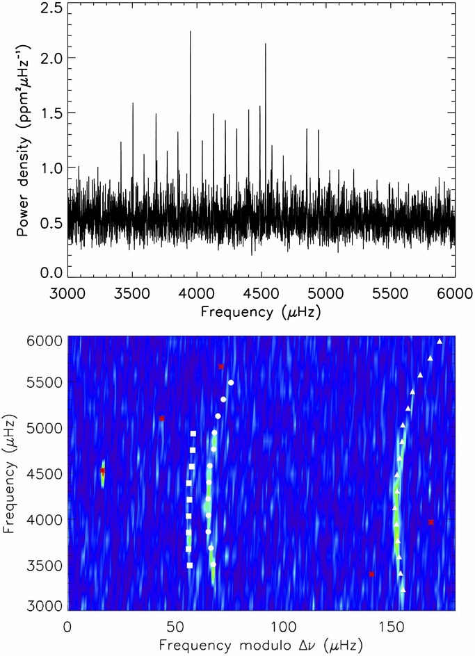
Mode frequencies were extracted from the power spectrum using a Markov Chain Monte Carlo (MCMC) fitting procedure (Handberg & Campante 2011; Campante 2012). Mode frequency posterior probability distributions are typically well described by a normal distribution, so we report the median of the distribution together with the standard deviation representing the 68.3% credible region. Mode frequencies were corrected to account for the Doppler shift due to the line-of-sight motion of the star (Davies et al. 2014). The observed oscillation frequencies (both corrected and uncorrected) are listed in Table 3. Figure 7 shows the power spectrum of the flux time series of Kepler-444.

Figure 7. Top panel: frequency–power spectrum of the flux time series of Kepler-444 over the frequency range occupied by the solar-like oscillations. A boxcar filter of width 1.5 μHz has been applied to enhance p-mode visibility. Bottom panel: power spectrum of the Kepler light curve in échelle format. This is the graphical equivalent to slicing the spectrum into segments of length Δν = 179.64 μHz and stacking them one on top of the other. Note that, in order to center the power ridges on the diagram, frequencies have been shifted sideways by subtracting a fixed reference of 25.5 μHz (i.e.,  ). White symbols represent the observed oscillation frequencies. Symbol shapes indicate mode degree: l = 0 (circles), l = 1 (triangles), and l = 2 (squares). Red asterisks mark the harmonics of the inverse of the Kepler long-cadence period (Δt ∼ 30 minutes), not all of which are present in these data. These artifacts appear in the power spectra of Kepler short-cadence time series.
Download figure:
Standard image High-resolution imageTable 3. Observed Oscillation Frequencies
| Uncorrected | Corrected | |||
|---|---|---|---|---|
| l | Frequency | Uncertainty | Frequency | Uncertainty |
| (μHz) | (μHz) | (μHz)a | (μHz)a | |
| 0 | 3504.57 | 0.34 | 3503.16 | 0.30 |
| 0 | 3683.12 | 0.15 | 3681.62 | 0.19 |
| 0 | 3861.50 | 0.32 | 3859.95 | 0.32 |
| 0 | 4041.25 | 0.15 | 4039.61 | 0.19 |
| 0 | 4220.76 | 0.61 | 4218.94 | 0.65 |
| 0 | 4400.74 | 0.26 | 4398.93 | 0.27 |
| 0 | 4580.84 | 0.32 | 4578.97 | 0.33 |
| 0 | 4762.20 | 0.99 | 4760.56 | 0.97 |
| 0 | 4942.24 | 0.54 | 4940.25 | 0.48 |
| 0 | 5123.48 | 0.92 | 5121.34 | 0.91 |
| 0 | 5305.62 | 0.98 | 5303.53 | 0.95 |
| 0 | 5488.79 | 1.05 | 5486.60 | 1.06 |
| 1 | 3233.26 | 0.70 | 3231.90 | 0.66 |
| 1 | 3411.70 | 0.53 | 3410.31 | 0.52 |
| 1 | 3590.67 | 0.89 | 3589.17 | 0.79 |
| 1 | 3769.67 | 0.26 | 3768.14 | 0.27 |
| 1 | 3948.73 | 0.13 | 3947.13 | 0.12 |
| 1 | 4127.62 | 0.10 | 4125.94 | 0.07 |
| 1 | 4308.32 | 0.25 | 4306.58 | 0.28 |
| 1 | 4487.89 | 0.36 | 4486.01 | 0.40 |
| 1 | 4668.67 | 0.49 | 4666.76 | 0.46 |
| 1 | 4849.51 | 0.38 | 4847.53 | 0.35 |
| 1 | 5029.49 | 1.05 | 5027.48 | 1.09 |
| 1 | 5211.57 | 1.05 | 5209.39 | 1.06 |
| 1 | 5393.24 | 0.86 | 5391.18 | 0.87 |
| 1 | 5576.51 | 0.91 | 5574.40 | 0.92 |
| 1 | 5760.77 | 0.77 | 5758.44 | 0.78 |
| 1 | 5944.74 | 0.94 | 5942.30 | 0.99 |
| 2 | 3493.67 | 1.03 | 3492.23 | 0.97 |
| 2 | 3672.71 | 0.49 | 3671.21 | 0.52 |
| 2 | 3852.45 | 0.31 | 3850.81 | 0.27 |
| 2 | 4032.07 | 0.27 | 4030.45 | 0.24 |
| 2 | 4212.04 | 0.76 | 4210.38 | 0.76 |
| 2 | 4391.47 | 0.80 | 4389.74 | 0.77 |
| 2 | 4572.47 | 0.68 | 4570.62 | 0.66 |
| 2 | 4752.43 | 0.83 | 4750.56 | 0.80 |
| 2 | 4932.40 | 0.91 | 4930.32 | 0.91 |
Note. aThe correction for the line-of-sight Doppler velocity shift modifies the frequencies and associated uncertainties by multiplying these quantities with 1 + Vr/c, where Vr is the radial velocity and c is the speed of light (for further details, see Davies et al. 2014).
Download table as: ASCIITypeset image
Stellar properties were determined using three different techniques to model the oscillation frequencies extracted from the data. The first method relies on a dense grid of stellar models computed with the GARching STellar Evolution Code (GARSTEC; Weiss & Schlattl 2008) including the effects of microscopic diffusion, and on theoretical frequencies calculated using the Aarhus aDIabatic PuLSation code (Christensen-Dalsgaard 2008a). The results were obtained implementing a Bayesian scheme that uses the spectroscopic constraints and frequency ratios as the parameters in the fit (V. Silva Aguirre et al., submitted), the latter being almost insensitive to the surface effects in solar-like oscillators (Roxburgh & Vorontsov 2003; Silva Aguirre et al. 2011). Central values are given as the estimates of the stellar properties obtained in this manner. We also computed models using the ASTEC and YREC codes. In these cases, the fit was made to the individual frequencies after correcting for the surface effect with, respectively, an appropriately scaled version of the observed solar surface correction (Christensen-Dalsgaard 2012) and a solar-type correction as described in Carter et al. (2012). The stellar properties derived using the three techniques described above are consistent within the returned formal errors. Therefore, we added in quadrature the difference in central values of each property to the formal uncertainties determined from the GARSTEC Bayesian scheme as a measurement of the systematic spread arising from different codes and fitting techniques. In Table 2, we provide a precise estimate of the stellar age, t, from detailed frequency modeling. Values for the remaining fundamental stellar properties are consistent, within errors, with those obtained from grid-based modeling. In particular, no gain in precision was obtained for the stellar radius. On the other hand, the precision on the stellar mass is improved by nearly a factor of two, from 5.7% to 3.2%.
5. CHARACTERIZATION OF THE PLANETARY SYSTEM
5.1. Transit Analysis
We investigated the planetary and orbital properties of the Kepler-444 system using long-cadence Kepler data (Δt ∼ 30 miutes; Jenkins et al. 2010). These data virtually span the entire duration of the nominal mission, with approximately 4 yr of nearly continuous coverage. In order to limit biases induced by stellar variability and instrumental systematics, we high-pass filtered the data using a second-order Savitzky–Golay filter with a 2 day window. Data points in transit were assigned null weight in the filter to avoid diluting the transit signals. The filtering was performed independently for each quarter and the data were combined after normalizing the individual quarters to their median value.
We measured the properties of the five planets in a similar manner to that described in Rowe et al. (2014), who used the same transiting-planet model. The model includes all five planets, with transit shapes described by the analytic model of Mandel & Agol (2002) using a quadratic limb-darkening law. The transit model computes a full orbital solution for each of the planets, which allowed for eccentricity to vary. We fixed the dilution of the light curve at 3.94% based on our adaptive optics observations. Marginal transit-timing variations (TTVs) have been detected for the outermost planetary pair. Their amplitudes are, nevertheless, very small and do not affect the measured planetary and orbital parameters. The potential detection of TTVs in this system will be addressed in future work. Free parameters in the fit include the mean stellar density, 〈ρ〉, the two limb-darkening parameters, γ1 and γ2, and for each planet the time at the midpoint of the first transit, T0, the orbital period, P, the planet-to-star radius ratio, Rp/R⋆, the impact parameter, b, and the two eccentricity vectors esin ω and ecos ω, where e is the orbital eccentricity and ω is the argument of periastron.
The data were modeled using an affine-invariant ensemble MCMC algorithm that utilizes multiple chains to decrease autocorrelation time (Goodman & Weare 2010; Foreman-Mackey et al. 2013). The asteroseismically derived mean stellar density was used as a strong prior in the transit model, while the limb-darkening coefficients were constrained by a prior of width 0.1 and mean derived from the model limb-darkening coefficients for the Kepler bandpass (Claret & Bloemen 2011). Furthermore, both the mid-transit time and orbital period were assigned flat priors, a uniform prior in the range [0, 1] was adopted for the planet-to-star radius ratio, and the prior for the impact parameter was set to a uniform distribution in the range [0, 1 + Rp/R⋆] to allow for grazing transits. The eccentricity vectors were assigned uniform priors in the range [ − 1, 1], although we have included an 1/e correction which has the effect of enforcing a uniform prior in eccentricity (Eastman et al. 2013).
We used a Gaussian likelihood function in our MCMC analysis which takes the form of a chi-squared log-likelihood (Quintana et al. 2014). We work in log-likelihood space since it enhances numerical stability. We ran the MCMC with 600 chains and 30, 000 jumps of each chain, but discarded the first 10, 000 jumps as burn-in. The chains were all well mixed and converged upon a unimodal posterior distribution in each model parameter. In Table 4, we quote the median and associated 68.3% credible region for all measured (and derived) planetary and orbital parameters. The best-fitting model is shown, plotted over the phase-folded transit data, in Figure 8. The best-fitting model is based on the maximum a posteriori parameter estimates.

Figure 8. Transit light curves for the five planets orbiting Kepler-444. From panels (a) to (e): transits of planets Kepler-444b, Kepler-444c, Kepler-444d, Kepler-444e, and Kepler-444f, respectively. The photometric light curves have been phase-folded on the orbital period of the planets to show the observed data as a function of orbital phase. Individual data points are shown as gray dots. Blue dots correspond to a binning of individual data points, shown only for clarity. The magnitude of the associated error bars is then given by the standard deviation of the data making up each bin divided by the square root of the number of points in the bin. These error bars are comparable in size to the blue dots. The best-fitting transit model, based on the maximum a posteriori parameter estimates, is shown as a red line.
Download figure:
Standard image High-resolution imageTable 4. Planetary and Orbital Parameters
| Parameter | Kepler-444b | Kepler-444c | Kepler-444d | Kepler-444e | Kepler-444f |
|---|---|---|---|---|---|
| T0 (BJD − 2, 454, 833) |  |
 |
 |
 |
 |
| P (days) |  |
 |
 |
 |
 |
| Rp/R⋆ |  |
 |
 |
 |
 |
| Rp/R⊕ |  |
 |
 |
 |
 |
| b |  |
 |
 |
 |
 |
| esin ω |  |
 |
 |
 |
 |
| ecos ω |  |
 |
 |
 |
 |
| ea |  |
 |
 |
 |
 |
| a/R⋆ |  |
 |
 |
 |
 |
| a (AU) |  |
 |
 |
 |
 |
| i (deg) |  |
 |
 |
 |
 |
Notes. Besides the free parameters in the fit, we have also included the planet radius in Earth radii, Rp/R⊕, the eccentricity, e, the semi-major axis in stellar radii, a/R⋆, the semi-major axis, a, and the orbital inclination, i. aThe eccentricity has a non-Gaussian posterior distribution and so the median is an overestimate of the true eccentricity.
Download table as: ASCIITypeset image
5.2. System Validation
The five planet candidates associated with Kepler-444 constitute a true five-planet system orbiting the target star. In what follows we present several lines of evidence that support this conclusion.
We start by invoking statistical arguments to exclude the scenario in which one or more transit-like signals are caused by chance-alignment blends such as background eclipsing binaries. Background eclipsing binaries are the primary source for the occurrence of false positives among Kepler planet candidates. Therefore, it is reasonable to assume that false positives are randomly distributed among Kepler target stars. Moreover, the number of Kepler planet candidates in multiple systems is considerably larger than what would be expected if these were assigned randomly to target stars. These considerations prompted Lissauer et al. (2012) to devise a statistical approach for the validation of planet candidates in multiple systems. For a system with five planet candidates, the only plausible false-positive configuration would be that of four planets and one background eclipsing binary (Lissauer et al. 2012). Chances of that happening are of 0.07%, if we assume that the fraction of candidates that are planets (viz., the fidelity of the sample) takes the rather realistic value of 0.9. We thus exclude the possibility of a background eclipsing binary at the 99.9% level. The above statistical framework has been recently refined by using a larger, more uniform, and better vetted set of planet candidates (Lissauer et al. 2014). Once again, the only plausible false-positive configuration continues to be that of four planets and one background eclipsing binary. Assuming a fidelity of the sample of single-planet candidates (and not the overall fidelity of the sample as before) of 0.9, then the chances of that happening are of 0.10%, and we are still able to exclude the possibility of occurrence of false positives at the 99.9% level. Given the target star's high proper motion, a sanity check would be to look at Digitized Sky Survey28 POSS-I (epoch 1945–58) and POSS-II (epoch 1984–99) images of the region where Kepler-444 currently is and see whether there are any background stars (Figure 9). We can see that there are no background stars in the above region down to the confusion limit of the images (V ∼ 22).

Figure 9. Digitized Sky Survey POSS-I (left-hand panel) and POSS-II (right-hand panel) images of the region where Kepler-444 currently is. Open circles at the center of both images mark the target star's current position (J2000.0). Both images have a size of 4' × 4' and were taken in the red.
Download figure:
Standard image High-resolution imageWe now invoke the non-randomness of the observed multi-resonant chain (Fabrycky et al. 2014) to assert that all five planets form a single system orbiting the same star. Theoretical models of planet formation and migration suggest that there may be an excess of exoplanet pairs near mean-motion resonances (MMRs; Marcy et al. 2001; Terquem & Papaloizou 2007). Based on a statistical sample of 408 Kepler planet candidates in multiple systems, it has been shown that the number of planetary pairs in or near MMRs exceeds that of a random distribution (Lissauer et al. 2011b). Moreover, the same authors found the distribution of candidate period ratios to exhibit prominent spikes near strong MMRs, implying that candidates with such period ratios are likely to be true planets. This is the case of all adjacent pairs in the Kepler-444 system, whose period ratios are just wide of first-order MMRs, being nearly commensurate. By extension, the observed multi-resonant chain provides strong evidence that all five planets form a single system. We next quantify this assertion. For each adjacent pair, we computed the variable ζ1, 1, which measures the scaled difference between the observed period ratio and the first-order MMR in its neighborhood (Fabrycky et al. 2014). The null hypothesis being that near-resonant locations are not preferred, as would be the case if planet pairs did not orbit the same star, means that the sum ∑|ζ1, 1| over all adjacent pairs approximately follows an Irwin–Hall distribution.29 The probability that ∑|ζ1, 1| takes a value less than or equal to the one observed is then of about 7%. We thus reject the null hypothesis at the 90% level. This not only means that the observed multi-resonant chain is likely not just a product of chance, but also that the resonances played a role in shaping the system's architecture. We take this as a strong indication that all five planets form a single system orbiting the same star.
We further mention stability as a boost in our confidence that these are in fact genuine planets in a multiple system. In tightly packed high-multiplicity systems, most configurations sharing the same number of planets randomly spread over the same range in period are likely to be unstable (Lissauer et al. 2011b, 2012). Therefore, finding evidence of the system's stability will aid in its validation. We computed the nominal dynamical separation, Δ, between each adjacent pair having made use of a simple power-law mass–radius relationship (Lissauer et al. 2011b; Fabrycky et al. 2014). All dynamical separations satisfy the stability condition for two-planet systems (i.e.,  ) and are thus Hill stable (Gladman 1993). Furthermore, taking each adjacent set of three planets, the Δ separations of the inner (Δinner) and outer (Δouter) pairs satisfy the heuristic stability condition Δinner + Δouter > 18 (Lissauer et al. 2011b). This is taken as plausible evidence of the system's stability. Moreover, by enforcing marginal dynamical stability one requires that the five orbiting bodies are substellar in mass, thus validating their planetary nature. In this regard, we should add that determining the planetary masses from radial velocity measurements would be extremely challenging, the predicted semi-amplitude being K ≈ 0.3 m s−1 even with all five planets contributing.
Finally, we establish that the planets transit the target star and not one of its M-dwarf companions. Measurements of shifts in the Kepler pixel-mask photocenter during a transit have been used in previous studies to help identify transit sources that are separated from the target stars. However, for heavily saturated target stars such as Kepler-444, a centroid analysis is highly unreliable (Bryson et al. 2013). Therefore, we instead followed a different approach and tested the dynamical stability of the five planets if they were to all orbit either of the M dwarfs. Although the stellar parameters of the brighter M-dwarf companion are better constrained, both M dwarfs have similar properties (Teff ∼ 3500 K and log g ∼ 5 dex; Section 2.2), and so we adopted these values and assumed that each contributes the same amount of dilution (1.97%). We thus need only consider the case of planets orbiting one of these M dwarfs, since they are, for stability purposes, essentially the same. In this scenario, the M dwarf is 4.22 Kepler magnitudes fainter than the target K star, and by interpolating over Dartmouth (Dotter et al. 2008) stellar evolution isochrones (assuming primary and secondaries co-evolved), we derived a mass of 0.37 M☉ and a radius of 0.36 R☉ for the M dwarf. The semi-major axes of the planets were computed via Kepler's law using the precise orbital period measurements. The planetary radii were computed from Rp/R⋆, assuming a fixed dilution of 96.06% from the target K star and 1.97% from the other M dwarf, yielding (from the innermost to the outermost planet): 1.33, 1.64, 1.75, 1.80, and 2.45 R⊕. Because the planetary masses are unknown (regardless of which star they orbit), we estimated their masses for an exhaustive range of compositional schemes using mass–radius relations derived from theoretical thermal evolution models (Fortney et al. 2007; Lopez et al. 2012). We examined the dynamical stability for planets composed of different mixtures of ice (low-density, less massive planets), as well as of silicate rock and iron (high-density, more massive planets). We also included 1% (by mass) H/He gas envelopes, certainly pertinent to planets larger than about 1.7–2 R⊕ as these may be mini-Neptunes rather than super-Earths with solid surfaces, although planets this close to their star (within 0.06 AU in this scenario) are highly irradiated and would thus be vulnerable to atmospheric escape (Lopez et al. 2012). For all compositional schemes tested, the planets became unstable within 102 to several 103 yr, even in the extremely unlikely case of pure ice planets. These results decisively support the competing scenario that the planets orbit the target K dwarf. We thus conclude that the five planet candidates associated with Kepler-444 constitute a true five-planet system orbiting the target K star.
6. DISCUSSION AND CONCLUSIONS
The precision with which we measured the planetary radii varies between 2.9% and 5.5%. Kepler-444b is the innermost and smallest planet (within 2σ of the size of Mercury). Its radius was measured with a precision of ∼100 km. All five planets are sub-Earth-sized with monotonically increasing radii as a function of orbital distance: 0.403, 0.497, 0.530, 0.546, and 0.741 R⊕. Kepler-444c, Kepler-444d, and Kepler-444e have very similar radii, respectively within 2σ, 1σ, and 1σ of the size of Mars. Finally, Kepler-444f has a size intermediate to Mars and Venus. Kepler-444 thus expands the population of planets found in low-metallicity environments from the mini-Neptunes around Galactic halo's Kapteyn's star (Anglada-Escudé et al. 2014) down to the regime of terrestrial-size planets. Although photometry alone does not yield the masses of the planets, planetary thermal evolution models (Lopez & Fortney 2014) predict that the composition of planets with radii less than 0.8 R⊕ are highly likely rocky.
The parent star, and hence the planetary system, has an age of 11.2 ± 1.0 Gyr from detailed frequency modeling. Kepler-444 is slightly older than Kepler-10, the host of two rocky super-Earths (Batalha et al. 2011; Dumusque et al. 2014), whose age of 10.4 ± 1.4 Gyr has also been determined from a detailed modeling of the oscillation frequencies (Fogtmann-Schulz et al. 2014). The precision with which the age of Kepler-444 has been determined from asteroseismology (∼9%) is an impressive technical achievement that was only made possible due to the extended and high-quality photometry provided by the Kepler mission. We have thus attained the level of precision expected for ESA's future PLATO mission, which has the science goal of providing stellar ages to 10% precision as a key to exoplanet parameter accuracy (Rauer et al. 2014). The estimated stellar age is commensurate with the ages of thick-disk field stars, which are older than about 10–11 Gyr (Reddy et al. 2006). It is also in general good agreement with several studies of the Arcturus stream based on different selections of stream members (Navarro et al. 2004; Helmi et al. 2006; Williams et al. 2009; Ramya et al. 2012). In Ramya et al. (2012), stellar ages were determined for a selection of stream members based on their location in a color–magnitude diagram. Ages of stream members were seen to vary between 10 and 14 Gyr. An individual age estimate for Kepler-444 was given by  , thus being significantly greater than the asteroseismic age estimate. Kepler-444 is the oldest known system of terrestrial-size planets. We thus show that Earth-size planets have formed throughout most of the universe's 13.8 billion year history, providing scope for the existence of ancient life in the Galaxy. Remarkably, by the time Earth formed, this star and its Earth-size companions were already older than our planet is today.
This system is highly compact, both in terms of its architecture and in a dynamical sense. All planets orbit the parent star in less than 10 days, or within 0.08 AU, roughly one-fifth the size of Mercury's orbit. These orbits are well interior to the inner edge of the system's habitable zone, which lies 0.47 AU from the parent star if we consider the rather optimistic "Recent Venus" limit of Kopparapu et al. (2013). Also, the orbits of the planets are consistent with having zero mutual inclinations, an indication of near-coplanarity. Furthermore, all adjacent planet pairs are close to being in exact orbital resonances, with period ratios no more than ∼2% in excess of strong 5: 4, 4: 3, 5: 4, and 5: 4 first-order MMRs as one moves toward the outermost pair. This latter feature could potentially facilitate the determination of the planetary masses via TTVs (e.g., Wu & Lithwick 2013). Other highly compact multiple-planet systems—characterized by a concentration of dynamically packed planets near 0.1 AU—include, e.g., Kepler-11 (Lissauer et al. 2011a), Kepler-32 (Swift et al. 2013), Kepler-33 (Lissauer et al. 2012), and Kepler-80 (Rowe et al. 2014), all with at least five planets (Figure 10). Kepler-444 is thus a member of a distinct population of highly compact planetary systems, which make up only ∼1% of all Kepler targets with planetary candidates (Lissauer et al. 2011b).

Figure 10. Semi-major axes of planets belonging to the highly compact multiple-planet systems Kepler-444, Kepler-11, Kepler-32, Kepler-33, and Kepler-80. Semi-major axes of planets in the solar system are shown for comparison. The vertical dotted line marks the semi-major axis of Mercury. Symbol size is proportional to planetary radius. Note that all planets in the Kepler-444 system are interior to the orbit of the innermost planet in the Kepler-11 system, the prototype of this class of highly compact multiple-planet systems.
Download figure:
Standard image High-resolution image
The proximity of each planet to a strong, first-order MMR indicates that this system evolved dynamically after the formation of the planets. A likely mechanism to produce such a configuration is convergent inward migration within a gaseous or planetesimal disk. Since these planets are all sub-Earth-sized and likely of similar composition (Weiss & Marcy 2014), the monotonic increase in planetary size as a function of orbital distance would imply that the masses of the planets increase outward. This would provide a means for convergent migration, since the migration rate is expected to scale as planet mass (Kley & Nelson 2012). The subsequent damping of orbital eccentricities as a result of tidal evolution would tend to spread the orbits, pushing them wide of exact commensurability as observed.
In addition to the dynamical evolution, the chemical environment is thought to play a decisive role in the formation of systems of terrestrial-size planets such as Kepler-444. While gas-giant planets appear to form preferentially around metal-rich stars, small planets (with radii less than 4 R⊕) can form under a wide range of metallicities (Sousa et al. 2011; Buchhave et al. 2012, 2014). This could mean that the process of formation of small, including Earth-size, planets is less selective than that of gas giants, with the former likely starting to form at an earlier epoch in the universe's history when metals were far less abundant (Fischer 2012). There is growing evidence that the critical elements for planet formation in iron-poor environments are α-process elements (Cochran et al. 2008; Brugamyer et al. 2011; Adibekyan et al. 2012a). In particular, α elements comprise the bulk of the material that constitutes rocky, Earth-size planets (Valencia et al. 2007, 2010). Stars belonging to the thick disk are overabundant in α elements compared to thin-disk stars in the low-metallicity regime (Reddy et al. 2006), which may explain the greater planet incidence among thick-disk stars for metallicities below half that of the Sun (Adibekyan et al. 2012b). Similarly favorable conditions to planet formation in iron-poor environments seem to be associated with a fraction of the halo stellar population, namely, the so-called high-α stars (Nissen & Schuster 2010). Thus, thick-disk and high-α halo stars were likely hosts to the first Galactic planets. The discovery of an ancient system of terrestrial-size planets around the thick-disk star Kepler-444 confirms that the first planets formed very early in the history of the Galaxy, thus helping to pinpoint the beginning of the era of planet formation.
The first discoveries of exoplanets around Sun-like stars (Mayor & Queloz 1995; Marcy & Butler 1996) have fueled efforts to find ever smaller worlds evocative of Earth and other terrestrial planets in the solar system. From the first rocky exoplanets (Queloz et al. 2009; Batalha et al. 2011) to the discovery of an Earth-size planet orbiting another star in its habitable zone (Quintana et al. 2014), we are now getting first glimpses of the variety of Galactic environments conducive to the formation of these small worlds. As a result, the path toward a more complete understanding of early planet formation in the Galaxy starts unfolding before us.
Funding for the Kepler mission is provided by NASA's Science Mission Directorate. The authors thank the entire Kepler team, without whom these results would not be possible. We thank David W. Latham for helpful comments on the manuscript. Funding for the Stellar Astrophysics Centre is provided by The Danish National Research Foundation (grant DNRF106). The research is supported by the ASTERISK project (ASTERoseismic Investigations with SONG and Kepler) funded by the European Research Council (grant agreement No. 267864). The research leading to the presented results has received funding from the European Research Council under the European Community's Seventh Framework Programme (FP7/2007-2013)/ERC grant agreement No. 338251 (StellarAges). This research made use of APLpy, an open-source plotting package for Python hosted at http://aplpy.github.com. T.L.C., G.R.D., W.J.C., R.H., A.M., and Y.P.E. acknowledge the support of the UK Science and Technology Facilities Council (STFC). T.B. was supported by a NASA Keck PI Data Award, administered by the NASA Exoplanet Science Institute. Some of the data presented herein were obtained at the W. M. Keck Observatory from telescope time allocated to the National Aeronautics and Space Administration through the agency's scientific partnership with the California Institute of Technology and the University of California. The Observatory was made possible by the generous financial support of the W. M. Keck Foundation. The authors wish to recognize and acknowledge the very significant cultural role and reverence that the summit of Mauna Kea has always had within the indigenous Hawaiian community. We are most fortunate to have the opportunity to conduct observations from this mountain. D.H. and E.V.Q. acknowledge support by an appointment to the NASA Postdoctoral Program at Ames Research Center administered by Oak Ridge Associated Universities. D.H. also acknowledges NASA grant NNX14AB92G issued through the Kepler Participating Scientist Program and support by the Australian Research Council's Discovery Projects funding scheme (project No. DE40101364). V.Zh.A., N.C.S., and S.G.S. acknowledge support from the European Research Council/European Community under FP7 through Starting grant agreement No. 239953, and from FCT (Portugal) through FEDER funds in program COMPETE, as well as through national funds in the form of grants RECI/FIS-AST/0176/2012 (FCOMP-01-0124-FEDER-027493) and RECI/FIS-AST/0163/2012 (FCOMP-01-0124-FEDER-027492). V.Zh.A. and S.G.S. also acknowledge grants SFRH/BPD/70574/2010 and SFRH/BPD/47611/2008 from FCT (Portugal), respectively. The Robo-AO system is supported by collaborating partner institutions, the California Institute of Technology and the Inter-University Centre for Astronomy and Astrophysics, and by the National Science Foundation under grant Nos. AST-0906060 and AST-0960343, by the Mount Cuba Astronomical Foundation, and by a gift from Samuel Oschin. C.B. acknowledges support from the Alfred P. Sloan Foundation. S.B. acknowledges NSF grant AST-1105930 and NASA grant NNX13AE70G. T.S.M. acknowledges NASA grant NNX13AE91G. C.K. acknowledges support from the Villum Foundation. N.C.S. also acknowledges support in the form of contract reference IF/00169/2012 funded by FCT/MCTES (Portugal) and POPH/FSE (EC).
Facilities: Kepler - The Kepler Mission, Keck:I (HIRES) - KECK I Telescope, Keck:II (NIRC2) - KECK II Telescope, PO:1.5m (Robo-AO) - Palomar Observatory's 1.5 meter Telescope
Footnotes
- 26
- 27
- 28
- 29
The Irwin–Hall distribution is the probability distribution of a random variable defined as the sum of a number of independent random variables, each having a uniform distribution.