


ABSTRACT
Since the unusually prolonged and weak solar minimum between solar cycles 23 and 24 (2008–2010), the sunspot number is smaller and the overall morphology of the Sun's magnetic field is more complicated (i.e., less of a dipole component and more of a tilted current sheet) compared with the same minimum and ascending phases of the previous cycle. Nearly 13 yr after the last solar maximum (∼2000), the monthly sunspot number is currently only at half the highest value of the past cycle's maximum, whereas the polar magnetic field of the Sun is reversing (north pole first). These circumstances make it timely to consider alternatives to the sunspot number for tracking the Sun's magnetic cycle and measuring its complexity. In this study, we introduce two novel parameters, the standard deviation (SD) of the latitude of the heliospheric current sheet (HCS) and the integrated slope (SL) of the HCS, to evaluate the complexity of the Sun's magnetic field and track the solar cycle. SD and SL are obtained from the magnetic synoptic maps calculated by a potential field source surface model. We find that SD and SL are sensitive to the complexity of the HCS: (1) they have low values when the HCS is flat at solar minimum, and high values when the HCS is highly tilted at solar maximum; (2) they respond to the topology of the HCS differently, as a higher SD value indicates that a larger part of the HCS extends to higher latitude, while a higher SL value implies that the HCS is wavier; (3) they are good indicators of magnetically anomalous cycles. Based on the comparison between SD and SL with the normalized sunspot number in the most recent four solar cycles, we find that in 2011 the solar magnetic field had attained a similar complexity as compared to the previous maxima. In addition, in the ascending phase of cycle 24, SD and SL in the northern hemisphere were on the average much greater than in the southern hemisphere, indicating a more tilted and wavier HCS in the north than the south, associated with the early reversal of the polar magnetic field in the north relative to the south.
Export citation and abstract BibTeX RIS
1. INTRODUCTION
The open magnetic field, with one end attached to the Sun and the other end extending into the heliosphere, expands non-radially (Banaszkiewicz et al. 1998) such that oppositely directed polarities come together at the equatorial plane at distances of several solar radii (Rs). On that plane, the curl of the magnetic field induces an electric current, creating the so-called heliospheric current sheet (HCS; Parker 1958). At solar minimum, the open magnetic field is well organized, with one polarity from each pole, and the HCS is a relatively flat surface centered on the Sun's ecliptic plane (Babcock 1961; Wang & Sheeley 2002; Forsyth et al. 1996; Bravo & Stewart 1996; Burlaga & Ness 1996). In the ascending phase to the solar maximum, polar coronal holes shrink and eventually vanish, and more coronal holes emerge at low latitudes in the Sun, whose magnetic field lines result in a highly inclined HCS (McComas et al. 2000; Riley et al. 2002). At solar maximum, the HCS reaches its maximum tilt and most disordered stage, and the Sun's polar polarity reversal usually occurs (Balogh & Smith 2001; Smith et al. 2001).
The flipping of the Sun's magnetic polarity usually takes place around solar maximum, recurring about every 11 yr, when the sunspot number is at its local maximum level (Vecchio et al. 2012; Jones et al. 2003; Hakamada 2013). However, the polar reversal is not necessarily temporally coincident with the absolute maximum in sunspot number, and indeed, solar maximum is not well defined as a particular time. It is very common that there are double peaks of sunspot numbers in one cycle (i.e., cycle 23 and 24). Also, the amplitude of sunspot maximum has varied from 50 to 250 in the past 24 cycles, i.e., the approximately 264 yr period during which sunspot numbers have been systematically recorded (Barnhart & Eichinger 2011). The variable—and one-dimensional—sunspot number is ultimately limited in its ability to quantify the complexity of the Sun's three-dimensional magnetic field.
The recent solar minimum (between solar cycles 23 and 24; 2008–2010) had fewer sunspots and was a prolonged minimum compared with previous minima (Vaquero et al. 2011; de Toma et al. 2010; Gibson et al. 2011). The Sun's open magnetic field was decreased by about 30% (Smith & Balogh 2008), the solar wind mass flux was decreased by 20% (McComas et al. 2008), and the corona was colder (Zhao & Fisk 2011; Lepri et al. 2013) than during the last minimum (cycles 22–23). Based on these observations, it has been predicted that the next solar cycle will also diverge from the norm, with a weaker and delayed solar maximum (Ramesh & Lakshmi 2012). In weighing the significance of such predictions, it is important to make use of as reliable and invariant criteria as possible for evaluating the complexity of the magnetic field of the Sun and the solar magnetic cycle.
It is the purpose of this paper to introduce a pair of new parameters, the standard deviation (SD) of the latitude of the HCS and the integrated slope (SL) of the HCS, to evaluate the global complexity of the Sun's magnetic field. These parameters can also be thought of as auxiliary methods for tracking the Sun's magnetic cycle. In Section 2, we introduce these parameters and discuss their sensitivity to the topology of the HCS. In Section 3, we compare them with the sunspot number using the recent four solar cycles as our test bed. Based on our evaluation, we suggest that in 2011 the solar magnetic field already reached the same complicated status as it was at the previous maxima. In Section 4, by using SL and SD, we evaluate the asymmetry of the magnetic field in the two hemispheres in the recent four ascending phases and find a clear asymmetry in cycle 24. In Section 5, we present our conclusions and a discussion.
2. INTRODUCING SD AND SL
2.1. Definition of SD and SL
Since the amplitude of the sunspot number at solar maximum is highly solar-cycle dependent and the properties (e.g., density, temperature, etc.) of the solar wind also change from cycle to cycle, these factors are limited in their ability to quantify the global variance of the Sun's magnetic field across solar cycles. An arguably more robust measure, whose cycle dependence has not been recorded to change since space data have been available, is the reversal of the solar polar field polarity as measured through the inclination of the HCS. The HCS is always relatively flat at solar minimum (Figure 1(a)) and very tilted at solar maximum, when the Sun's magnetic field is turning over (Cliver & Ling 2001; Hoeksema 1995; Figure 1(b)). This invariant cycle dependence of the HCS leads us to introduce a pair of new parameters that are independent of the sunspot number but are very efficient at tracking the complexity of the solar magnetic field as manifested in the HCS.
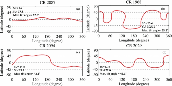
Figure 1. HCS curves on the 2.5 Rs surface are calculated from photospheric field observations with a potential field source surface (PFSS) model, shown by solid lines at (a) solar minimum, 2009 September, Carrington rotation 2087 and (b) solar maximum, 2000 October, Carrington rotation 1968, (c) ascending phase, 2010 March, Carrington rotation 2094, and (d) descending phase, 2005 April, Carrington rotation 2029. (Data were obtained at the Wilcox Solar Observatory: http://wso.stanford.edu/synsourcel.html).
Download figure:
Standard image High-resolution imageTo mathematically describe the different shapes of the HCS at different solar activity phases, we introduce two parameters: the latitudinal standard deviation (SD) and the integrated slope (SL) of the HCS. We define the SD as the standard deviation of the absolute values of the HCS' latitudes on the source surface for one Carrington rotation (CR; Equation (1)); SL is the total absolute value of the slope between two neighboring simulated points of the HCS on the source surface for one CR, or, in other words, the total absolute value of the derivative of the HCS' latitude with respect to longitude (Equation (2)). The definition of these two parameters can be analytically described as

where θi (ϕi) is heliographic latitude (longitude) of an HCS simulation point on the synoptic map, and  is the average of θi over the entire CR. In this study, we calculate these two parameters from the curve of the HCS on the synoptic Carrington maps provided by the potential field source surface (PFSS) model (Wang & Sheeley 1992) at the source surface of 2.5 Rs (Figure 1).
2.2. Using SD and SL to Evaluate the Complexity of the HCS
An example of how SD and SL describe the shape of the HCS is shown in Figure 1. In this figure, the polarity inversion line at 2.5 Rs is calculated from photospheric field observations as a boundary condition with a PFSS model (i.e., Wang & Sheeley 1990) and is shown by a red solid line, which can be used as an indicator of the HCS. As described above, the cycle dependence of the HCS is obvious: at solar minimum, very small values of SD and SL indicate that the HCS is more or less a flat sheet around the ecliptic plane (Figure 1(a)), whereas at solar maximum the HCS is tilted to high latitude (>60°) and its increased waviness corresponds to much higher values of SD and SL (Figure 1(b)).
A similar parameter based on the HCS calculated by the PFSS model, i.e., the maximum extent in latitude reached by HCS in one CR, or, in short, the maximum tilt angle, has also been used to track solar cycle variation (Cliver & Ling 2001). However, this parameter has limitations compared to SD and SL. For example, since the magnetic field lines are not computed above 70° by the PFSS model, the maximum tilt angle of the HCS above 70° is ill-defined. This limitation is especially problematic at solar maxima when the HCS commonly reaches latitudes > 70°. SD and SL, depending upon the behavior of the HCS throughout the CR, continue to provide meaningful distinctions from rotation to rotation even when the maximum tilt angle has essentially saturated at 70°. Also, the maximum tilt angle cannot evaluate the three-dimensional shape of the HCS, as it measures only a single number per rotation, i.e., the maximum latitudinal extent. On the other hand, SD and SL provide a global overall estimation about the inclination of the HCS and the complexity of its shape, which yields more information. This is illustrated in Figures 1(c) (CR2094) and 1(d) (CR2029): the two CRs have the same maximum tilt angle, but they have very different HCS shapes—CR2094's curve is more gradual, characterized by a relatively smaller SL but larger SD (Figure 1(c)) and CR2029 is much wavier, resulting in a relatively larger SL but smaller SD (Figure 1(d)).
3. USING SD AND SL TO EVALUATE THE ANOMALOUS CYCLE 23 AND 24
3.1. Comparison with the Sunspot Number
A comparison of SD and SL with monthly sunspot numbers is shown in Figure 2, where the sunspot numbers are plotted versus time from 1975 January to 2012 December. Monthly sunspot numbers (http://sidc.oma.be/sunspot-data/) are depicted by gray shading and SD (SL) is plotted in red (blue). This figure shows that both SD and SL vary with time in a similar way as the sunspot number does, and follow the same 11 yr cycle. However, quantitatively, these two parameters do not follow the sunspot number consistently, for two reasons. First, while the range of sunspot numbers can change significantly from cycle to cycle, the values of SD and SL oscillate within a constant range. Second, starting from the descending and minimum phases of cycle 23 (from 2003), the sunspot number showed an unusually slowly decreasing slope until reaching a very deep minimum in 2009. During this descending phase, SD and SL showed larger deviations from the sunspot number and stayed at higher levels than any same phase in the previous cycles shown in Figure 2, implying that the global magnetic field of the Sun was behaving differently than in previous cycles. This difference indeed is associated with the unusual solar minimum in 2008–2010, when the HCS was much more tilted and low-latitude coronal holes were more common than in the previous minima. The dramatic difference in SD and SL in the descending phase of cycle 23 makes this cycle stand out from the previous cycles, and since this difference occurred a few years before the sunspot number anomaly became apparent, it can be considered an early warning that the minimum between cycle 23 and 24 would be abnormal and—possibly—that cycle 24 will also be magnetically different.

Figure 2. Comparison of the monthly sunspot number (SSN), SD, and SL, from 1975 January to 2012 December. SSN is represented by the gray shading and SD (SL) is plotted as a red (blue) solid line. (Monthly SSN data were downloaded from http://sidc.oma.be/sunspot-data/). The SD values are scaled by 10 to fit on the same y-axis on the left.
Download figure:
Standard image High-resolution imageAfter 260 spotless days in 2009 (Zięba & Nieckarz 2012), sunspots gradually returned. In 2012, sunspots slowly climbed to about half of their historic maximum value from previous cycles. However, unlike the sunspot number, SD and SL increased at a similar rate as they did in previous solar cycles, and returned to their normal historic maximum levels in 2011, while the sunspot number was still only halfway to its peak reached in cycles 21–23. Again, this distinction between the sunspot number and the SD and SL parameters may indicate that cycle 24 will be magnetically different than the cycles of recent history. Also, the fact that SD and SL have reached their usual maximum values seems to suggest that the sunspot number also has reached the maximum for this cycle. Thus, SD and SL might also give an early warning of the cycle maximum, although we only have three cycles to support this statement and more would be needed.
3.2. Comparison with the Normalized Sunspot Number
Since the sunspot number is qualitatively periodic but quantitatively highly cycle dependent, as shown in Figure 2, we calculate the normalized sunspot number in each cycle and compare it with SD and SL (Figure 3). The normalized sunspot number is defined as the sunspot number divided by its maximum value in each cycle and is plotted versus the years after the beginning of each cycle in Figure 3. Note that for cycle 24, we use the maximum monthly sunspot number so far, which is 96.7 recorded in November 2011. The start date of each cycle that we use in this paper is from Owens et al. (2011), who defined the start date as the moment when the average latitude of sunspots sharply increases (Table 1). Figure 3(a) shows that in the recent four cycles (cycles 21–24), the normalized sunspot numbers all reach 0.8 (horizontal dashed line in Figure 3(a)) at about 2.5 yr (vertical dashed lines) after the beginning of the cycle. Therefore, if we define the solar maximum phase as the period when the normalized sunspot number is greater than 0.8, then the solar maxima in the four cycles all began about 2.5 yr after the start dates of the cycles.

Figure 3. Time plots of the normalized sunspot number (a), SD (b), SL (c), and smoothed SL (d) in the most recent four cycles. The horizontal dashed line in (a) indicates where the normalized sunspot number is 0.8, which is considered as a threshold of the onset of solar maxima in these four cycles. The horizontal dashed line in (b) marks where SD = 20 and in (c) and (d) marks where SL = 363, which can also be considered as a threshold for the onset of solar maximum. The vertical dashed lines mark 2.5 yr after the beginning of each cycle.
Download figure:
Standard image High-resolution imageTable 1. Start Dates and Onsets of Maxima in the Four Recent Solar Cycles
| Cycle 21 | Cycle 22 | Cycle 23 | Cycle 24 | |
|---|---|---|---|---|
| Start date of the cyclea | 1976.6 | 1986.7 | 1996.8 | 2009.0 |
| Onset of maximum | 1979.1 | 1989.2 | 1999.3 | 2011.5 |
Note. aOwens et al. (2011).
Download table as: ASCIITypeset image
Similarly, after 2.5 yr from the start date of the cycles, SD also reaches its maximum level (SD > 20, marked by the horizontal dashed line in Figure 3(b)). However, since SL is nosier than SD throughout all the cycles, there is no clear threshold of SL consistent with the onset of solar maximum (Figure 3(c)). Instead of using SL itself, we average SL every 10 months and find that the smoothed SL reaches a high level of 363 2.5 yr after the start date of each cycle (Figure 3(d)). These high values of SD and SL (SD > 20 and SL > 363) indicate that the HCS is highly tilted and wavy, which implies that the polar field is about to flip. This time period also marks the solar maximum. The coincidence of the high values of SD and SL and the maximum level of the normalized sunspot number suggests that SD and SL can be used as proxies for indicating the onset of solar maximum, in terms of magnetic field complexity. The onset dates of the recent four solar maxima determined from Figure 3 are tabulated in Table 1.
Note that the advantage of SD and SL in capturing the magnetic anomalous cycle is clearly illustrated in Figure 3. In Figure 3(a), even though the normalized sunspot numbers show a prolonged (unusual) solar minimum of cycle 23, this anomaly was not clear until the long minimum was underway. In contrast, the descending and minimum phases of cycle 23 clearly stand out from the other cycles in terms of the enhanced values of SD and SL in Figures 3(b)–(d). The enhanced SD and SL indicate that the HCS was much more tilted and extended to much higher latitude than it was in the previous cycles, implying that the global three-dimensional morphology of the Sun's magnetic field at this time was definitely different from past normal cycles. Indeed, this is evident by the higher rate of appearance of low-latitude coronal holes and pseudostreamer structures at that time (Zhao & Fisk 2011; Zhao et al. 2013). Also, note that the anomalous behavior of SD and SL was apparent already in 2003, while the anomaly of the minimum became obvious many years later. Thus, SD and SL seem to be giving early warnings of the anomalies of the HCS and the magnetic field.
It is also interesting to note that during the ascending phase (2009–2011) of cycle 24, when the sunspot number was so low compared with the ascending phases in the previous cycles (Figure 2), the SD and SL behaved similarly to the other three cycles (Figures 3(b)–(d)). This fact implies that if cycle 24 is unusual (Ramesh & Lakshmi 2012), it may become apparent in the SD and SL during the descending or minimum phase of cycle 24, in a way that will not be apparent in the sunspot number.
4. ASYMMETRY OF THE MAGNETIC FIELD IN THE TWO HEMISPHERES
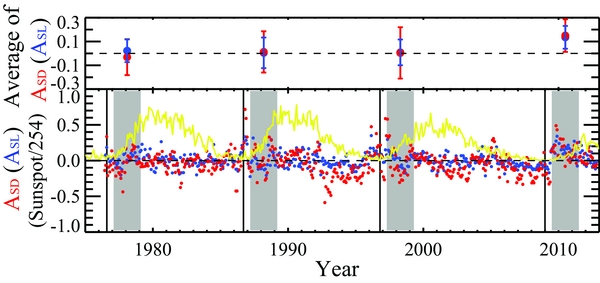
The asymmetry of the solar polar field reversal during solar maximum was first noticed in cycle 19 (Babcock 1959) when the south polar field reversed its polarity about one year earlier than the north pole did. This asymmetry is very clear again in cycle 24, as the negative magnetic field in the north pole has finished its reversal much earlier than the south pole (Hoeksema 2012; Shiota et al. 2012; Altrock 2012; Gopalswamy et al. 2012; Petrie 2012). We modify the definition of the parameter A, used by Chowdhury & Dwivedi (2011), to check if there is also an obvious north–south asymmetry in the parameters SD and SL. The definitions of ASD and ASL are expressed in Equations (3) and (4):


where SDnorth (SDsouth) and SLnorth (SLsouth) are SD and SL calculated separately based on the HCS in the north (south) hemisphere. Note that it is another advantage of SD and SL that they can be separately evaluated for the north and south hemisphere. Basically, positive ASD and ASL values indicate that SD and SL are greater in the northern hemisphere than in the south, and vice versa. Time plots of ASD and ASL are shown in Figure 4 (bottom), with the sunspot number over-plotted in yellow. We then chose the ascending periods, 0.5–2.5 yr after the start date of the cycles, to evaluate the average behavior of ASD and ASL. We found that in the ascending phase of cycle 24, the averaged ASD and ASL values both show dominant positive components that indicate that SD and SL are greater in the north hemisphere than in the south. This result implies that the HCS is more tilted in the north than in the south in this time period (Figure 4, top). This could have been interpreted as an early sign that the north pole would finish its reversal sooner than the south pole, which turned out to be true a couple of years later (Hakamada 2013; Svalgaard & Kamide 2013). In the previous three cycles, the averaged ASD and ASL were around zero, indicating that the asymmetry of the solar polar field on average was not so clear as in cycle 24 (Svalgaard & Kamide 2013; Wang & Sheeley 2002).
Figure 4. Bottom: time plots of ASD (red) and ASL (blue). Sunspot number (yellow) indicates the solar cycle phase. Gray shading highlights the time periods (0.5–2.5 yr after the start date of the solar cycle) in the four ascending phases where ASD and ASL are averaged. Top: averaged ASD (red circles) and ASL (blue circles) in the four gray shaded periods; the standard deviations of ASD and ASL in these periods are shown as error bars.
Download figure:
Standard image High-resolution image
5. SUMMARY AND CONCLUSIONS
In this work, we proposed two new parameters, SD and SL, which have several advantages.
- 1.They can evaluate the global complexity of the Sun's magnetic field. SD and SL have low values when the HCS is flat at solar minimum and high values when the HCS is highly tilted at solar maximum. SD and SL respond to the topology of the HCS differently, since higher SD values indicate a larger part of the HCS extending to higher latitudes, while higher SL values imply that the HCS is wavier (Figure 1).
- 2.They can identify magnetically anomalous cycles. For example, during the descending and minimum phases of cycle 23, when the normalized sunspot number only showed a longer declining process than in the previous cycles, abnormally enhanced SD and SL values indicated that the HCS was much more tilted and wavier than the same phases in the previous cycles (Figures 2 and 3). Such an anomaly became apparent a few years earlier than the anomaly in the sunspot number.
- 3.They can be auxiliaries to the sunspot number in tracking the phase of solar activity. Both SD and SL track the solar cycle in a similar way to the sunspot number, but unlike the sunspot number, they are insensitive to the strength of each cycle itself. In fact, the absolute number of sunspots can change from cycle to cycle by a factor up to four as shown by historical records available from 1749, indicating a significant variation in the strength of solar cycles themselves; on the contrary, the values of SD and SL oscillate in each cycle within a fixed range regardless of the strength of any particular cycle. As the peaks of SD and SL (smoothed by 10 months) coincided with the maximum level of the normalized sunspot number in the recent four cycles, SD and SL can also be used to track the solar maximum. Based on these two parameters, the Sun entered its maximum magnetic complexity stage of solar cycle 24 in or around 2011 June.
- 4.They can indicate the asymmetry of the polar field reversal. A symmetry evaluation of SD and SL shows that in the ascending phase of cycle 24, SD and SL in the northern hemisphere are on average much greater than in the southern hemisphere, which confirms that the HCS is more tilted and much wavier in the north than the south, an early warning that the north polar field would be ready for its polarity reversal sooner than the south (Figure 4). Such an indication turned out to be true at the end of 2012 (Hakamada 2013; Svalgaard & Kamide 2013).
These properties of SD and SL make them very useful parameters to evaluate the global coronal complexity. The most interesting property of SD and SL is that they are affected by both the polar field and the active region field, and they can provide an interesting measurement of how these two factors are related versus time for a given cycle. Therefore, SD and SL can reveal the nature of the cyclical variance of the complexity of the Sun's magnetic field to a degree that the sunspot number alone cannot.
L.Z. thanks Deborah Eddy for her assistance in editing this paper. The work of L.Z. and E.L. was supported by NASA grant NNX11AC20G. The National Center for Atmospheric Research (UCAR) is supported by the National Science Foundation.