


ABSTRACT
Hierarchical structure formation theory is based on the notion that mergers drive galaxy evolution, so a considerable framework of semi-analytic models and N-body simulations has been constructed to calculate how mergers transform a growing galaxy. However, galaxy mergers are only one type of major dynamical interaction between halos—another class of encounter, a close flyby, has been largely ignored. We use cosmological N-body simulations to reconstruct the entire dynamical interaction history of dark matter halos. We present a careful method of identifying and tracking a dark matter halo which resolves the typical classes of anomalies that occur in N-body data. This technique allows us to robustly follow halos and several hierarchical levels of subhalos as they grow, dissolve, merge, and flyby one another—thereby constructing both a census of the dynamical interactions in a volume and an archive of the dynamical evolution of an individual halo. In addition to a census of mergers, our tool characterizes the frequency of close flyby interactions in the universe. We find that the number of close flyby interactions is comparable to, or even surpasses, the number of mergers for halo masses ≳ 1011 M☉ h−1 at z ≲ 2. Halo flybys occur so frequently to high-mass halos that they are continually perturbed, unable to reach a dynamical equilibrium. In particular, we find that Milky Way type halos undergo a similar number of flybys as mergers irrespective of mass ratio for z ≲ 2. We also find tentative evidence that at high redshift, z ≳ 14, flybys are as frequent as mergers. Our results suggest that close halo flybys can play an important role in the evolution of the earliest dark matter halos and their galaxies, and can still influence galaxy evolution at the present epoch. Our companion paper quantifies the effect of close flyby interactions on galaxies and their dark matter hosts.
Export citation and abstract BibTeX RIS
1. INTRODUCTION
In a ΛCDM universe, the smallest dark matter halos form first; bigger halos are then formed via successive mergers with smaller halos. Thus, mergers are instrumental in the formation and evolution of halos. Galaxy mergers are rare, punctuated events in a galaxy lifespan that nonetheless dramatically change it—from its morphology (e.g., Holmberg 1941; Toomre & Toomre 1972; Schweizer 1986; Barnes & Hernquist 1992, 1996; Mihos & Hernquist 1996; Moore et al. 1996; Springel & White 1999; Dubinski et al. 1999; Barnes 2002; Springel et al. 2005a; Cox et al. 2006; Hopkins et al. 2006; Robertson et al. 2006a, 2006b; Naab et al. 2006a, 2006b; Covington et al. 2008; Mo et al. 1998; Holley-Bockelmann & Richstone 2000; Barnes 2002) to its stellar population (e.g., Mihos & Hernquist 1994; Hernquist & Mihos 1995; Cox et al. 2008; Bekki 2008), to the evolution of the central supermassive black hole (e.g., Springel et al. 2005b; Hopkins et al. 2005, 2006; Micic et al. 2007; Younger et al. 2008; Micic et al. 2011). Consequently, merger rates have been studied extensively, both theoretically (e.g., Lacey & Cole 1993; Guo & White 2008; Genel et al. 2008, 2009) and observationally (e.g., Schweizer 1986; Roberts et al. 2002; Laine et al. 2003; Casasola et al. 2004; van Dokkum 2005; Bridge et al. 2007; Lin et al. 2008; Tacconi et al. 2008; Urrutia et al. 2008; Ryan et al. 2008). Collisionless cosmological N-body simulations can be used to measure halo merger rates, where a merger is defined to occur when a bound dark matter halo falls into another bound dark matter halo. Various simulations measuring such halo merger rates agree to within a factor of ∼2 (see Hopkins et al. 2010 for a discussion on merger rates from collisionless simulations). Galaxy merger rates can then be inferred from the subhalo mergers within a primary halo by assuming a Mhalo–Mgal relation (e.g., Guo & White 2008; Wetzel et al. 2009; Behroozi et al. 2010) or directly measured in hydrodynamic simulations (e.g., Maller et al. 2006; Simha et al. 2009). Observationally, merger rates are typically derived from close-pair counts—galaxies with small projected separations and relative velocities—and are globalized using an estimate of the lifetime or duration of the observed merger phase (Lotz et al. 2010).
Ultimately, galaxy mergers are successful in shaping galaxy properties because they cause a large perturbation within the potential. Even an orbiting satellite can distort the underlying smooth galaxy potential and produce observable effects. For example, the H i warp in the Milky Way (MW) disk may be tidally triggered by the Large Magellanic Cloud (Weinberg & Blitz 2006). However, one entire class of galaxy interactions also capable of causing such perturbations—galaxy flybys—has been largely ignored.
Unlike galaxy mergers where two galaxies combine into one remnant, flybys occur when two independent galaxy halos interpenetrate but detach at a later time; this can generate a rapid and large perturbation in each galaxy. We developed and tested a method to identify mergers and flybys between dark matter halos in cosmological simulations and to construct a full "interaction network" that assesses the past interaction history of any given halo. With this new tool, we are undertaking the first systematic study to quantify the frequency of flybys and their effect on galaxy evolution.
In this paper, we present our technique for determining the network of dynamical interactions for halos in an N-body simulation, and present a census of halo flybys and mergers in the universe. We discuss our simulation and halo-finding technique in Section 2. Section 3 describes our technique to identify halo flyby interactions, and to construct a halo interaction network. Section 4 presents the results, and Section 5 discusses the implications of flyby interactions and previews the next paper in the series. The Appendix (A.0 to A.2) covers our method of linking parent and child halos, including ways to mitigate common problems that plague this process.
2. SIMULATION TESTBED AND HALO IDENTIFICATION
We use a high-resolution, dark matter simulation with 10243 particles in a box of length 50 Mpc h−1 with WMAP-5 cosmological (Komatsu et al. 2009) parameters as a testbed to develop our technique. The initial particle distribution is obtained from a Zeldovich linear approximation at a starting redshift of z = 249 and is evolved using the adaptive tree-code, GADGET-2 (Springel et al. 2001b; Springel 2005). The dark matter particles have a fixed gravitational comoving softening length of 2.5 kpc h−1. We store 105 snapshots spaced logarithmically in scale factor, a = 1/(1 + z), from z = 20 to 0. This translates into a timing resolution ≲ 50 Myr for z ≳ 3 and ∼150 Myr for z ≲ 3. Since the fundamental mode goes nonlinear at z = 0, we will only present results up to z = 1 where the 50 Mpc h−1 box is still a representative cosmological volume.
In addition, we ran two simulations designed to explore the effect of mass and timing resolution on the flyby phenomenon. These two volumes, with 5123 and 10243 particles, respectively, have the same size and cosmology as our testbed simulation and were evolved from z = 249 to 1. The particles were drawn from identical phases, and with 161 snapshots total, had timing resolution better than 200 Myr.
To begin identifying halos, we first use a friends-of-friends (FOF) technique with a canonical linking length b = 0.2 (∼10 kpc h−1) (Davis et al. 1985). We require at least 20 particles (∼108 M☉ h−1) to define a halo, but our halo interaction network uses only those halos with greater than 100 particles; we discuss the effects of this limit in Appendix A.2. Subhalos (down to multiple hierarchy levels) are identified using the SUBFIND algorithm (Springel et al. 2001a). The SUBFIND algorithm identifies subhalos as bound structures around a density maxima.1 The remaining particles in the FOF halo are comprised of particles that are bound to the potential of the main halo but not bound to any subhalo. For the remainder of this paper, all references to the main or primary halo will mean this bound set of "background" particles. For details on the SUBFIND algorithm, we refer the reader to Springel et al. (2001a). We caution that SUBFIND, or any density-based halo extraction technique, only recovers subhalo masses enclosed within a region of higher subhalo density compared to the background (see Muldrew et al. 2011). Therefore, a subhalo will lose mass depending on the radial distance from the center of the main halo, i.e., the subhalo mass is only to be trusted modulo a density contrast. If we want a detailed look at the subhalo mass loss evolution, then we must carefully correct for this bias. Fortunately, at this stage we simply require the existence of the subhalo; we caution that there is one consequence of this bias that presents a challenge: in the most extreme case, a subhalo passing through the center of the main halo can disappear for multiple snapshots only to reappear later, where it can be mistaken for a new subhalo. We account for such missing subhalos while constructing the halo interaction network (see Appendix A.1). Since our focus is on flybys, we relegate most of the discussion of our technique to the Appendix (A.0 to A.2), including resolution tests and comparison to other techniques (A.3 and A.4).
3. TAXONOMY OF HALO DYNAMICS
In a collisionless simulation, dark matter halos can grow via mergers or through smooth accretion. They can also lose mass through dynamical interactions, such as flybys or three-body encounters (e.g., Sales et al. 2007; Ludlow et al. 2009); primary halos can even be stripped of entire subhalos. Halos close to the numerical resolution limit can disappear for multiple snapshots. A primary halo can fall into another primary halo and continue to survive as a subhalo that is subsequently stripped. Ideally, a robust account of a halo's dynamical past captures all such scenarios and produces a physically meaningful history for individual halos. In a nutshell, our halo interaction network attempts to capture all of these interactions. We construct our halo interaction network in a three-step fashion: (1) for every halo, we find the best child halo at some later snapshot (if it exists); (2) we trace the complete set of parent–children pairs through all snapshots to construct the halo network; and (3) using the phase space history, we characterize the type of interaction for each pair.
Capturing the rich history of interactions of dark matter halos requires identifying every possible interaction. Most of the interesting phenomena begin with a main halo falling into another main halo. Assuming that a secondary main halo falls into a primary main halo, the following outcomes are possible.
- 1.The secondary (now a subhalo) continues to orbit inside the main halo and ultimately disrupts inside that same main halo (merger started).
- 2.The secondary continues to orbit the primary halo and exists at z = 0 (merger completed).
- 3.The secondary merges with another subhalo inside the same primary halo (subhalo merger).
- 4.The primary main becomes a subhalo itself by merging with another halo. The secondary is now a sub-subhalo (merger).
- 5.The secondary halo enters and then detaches from the primary halo (grazing flyby).
- 6.Either the secondary or the primary disappear (transients).
It is also possible that a subhalo appears without ever having been a main halo. Based on our snapshot timing resolution work (see Appendix A.3), we find that these subhalos formed as main halos very close to the primary and merge in between snapshots.
An interaction begins the moment a halo changes its state, e.g., when a main halo becomes a subhalo of another main halo. We categorize each interacting pair of halos by tracking the behavior of the pair into the future. At the moment the encounter begins, we tag the interaction according to the encounter type. For instance, when a subhalo enters a primary and eventually disrupts inside it, the interaction is tagged as a merger. Along with this tag, we store the redshift of infall (when the subhalo first becomes part of the main) and the destruction redshift. Thus, we automatically get a duration for every interaction. In addition, we store the minimum separation between the subhalo and primary halo and the normalized radius at destruction—this allows us to take census of the galactocentric distances reached by any particular interaction as a function of primary mass, mass ratio, and infall redshift while accounting for the dynamic behavior of the primary halo.
Since we use the redshift of infall as interaction redshift, mergers and flybys in our simulation will occur well before any observable encounter-induced features within the galaxies. For instance, the peak in the merger rate occurs for z ∼ 5 (see Figure 4) instead of z ≈ 2 as found elsewhere (Madau et al. 1996; Ryan et al. 2008). Note, though, that this definition of recording a merger as the redshift of infall is in line with the techniques used in the literature to construct merger trees using FOF halos.
3.1. Examples of Halo Evolution within the Network
In Figure 1, we show the halo interaction network for two MW type halos of ∼1012 M☉ h−1 at redshift zero.2 These are two drastically different halos, even though they have the same mass at z = 0. The first halo formed at z = 9.3 and had a very active merger history; by z = 0, the assembly of this halo required 434 mergers. The second halo formed earlier, at z = 12.5, yet only required 111 mergers—a "quiet" evolution. Much of the mass in the quiet halo is assembled early through smooth accretion of dark matter; at z ∼ 5, the hectic halo has a mass of 2 × 10¹⁰ M☉ h−1 while the quiet halo is 10 times more massive. The hectic primary halo itself directly survives 77 mergers, while the quiet halo undergoes only 27. Such divergent pasts can leave an imprint on the structure and properties of the galaxies contained in these halos—in the star formation history, the morphology, and perhaps the central black hole mass. We will explore this topic in a separate paper (M. Sinha & K. Holley-Bockelmann, in preparation).
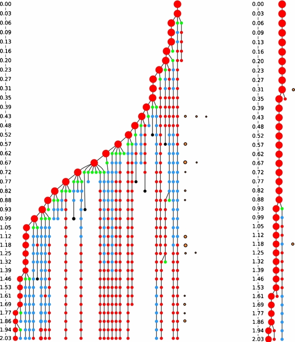
Figure 1. Left: merger tree for a hectic halo. The mass of the halo at z = 0 and z = 4.5 is 1.8 × 10¹² M☉ h−1 and 2 × 10¹⁰ M☉ h−1, respectively. Red represents a primary halo, blue represents a subhalo, green represents a subhalo that is going to dissolve inside the main halo, and black represents a halo that skips at least one snapshot. The size of the circle represents the halo's log-scaled mass with respect to the mass of the final main halo at z = 0. We only show those halos that are at least 1/10 of the primary mass. The corresponding redshifts are shown on the left. The flybys are shown on the right with yellow circles; the size of the circle is scaled to show the mass ratio of the flyby. The main halo undergoes 77 mergers and 21 flybys; however, we can only see a specific type of flyby in this merger tree—those relatively rare flybys that eventually result in a merger. Right: merger tree for a quiet MW mass halo. Flybys are shown as yellow circles on the right. If a subhalo actually survives until z = 0, then it will not appear in this merger tree. At z = 0, the halo mass is 1012 M☉ h−1, while at z = 4.5 it is 2 × 10¹¹ M☉ h−1; this halo assembled most of its mass early via smooth accretion.
Download figure:
Standard image High-resolution image3.2. Finding Flybys
One major goal of this paper is to characterize flyby interactions—interactions that do not end with one halo accreting another. In principle, there are three classes of close flyby interactions.
- 1.Grazing. Two primary halos approach on convergent trajectories, interpenetrate for at least half a crossing time, and then separate as two distinct primary halos once more.
- 2.External. Same as above but the primary halos remain distinct at all times. This can also apply to halos that are at the same hierarchy levels within the same container halo (e.g., two subhalos of the same main halo). Since technically this can include every other halo in the volume, it is useful to define a maximum pericenter distance between two halos when classifying this type.
- 3.Internal. A halo at a higher hierarchy level passes close to the center of its containing halo, e.g., a sub-sub halo goes through the central regions of its containing subhalo. This is synonymous with the decay of satellite orbits after a merger.
Internal flybys have been studied in great detail (e.g., Toth & Ostriker 1992; Quinn et al. 1993; Walker et al. 1996; Sellwood et al. 1998; Johnston 1998; Taylor & Babul 2001; Purcell et al. 2009; Kazantzidis et al. 2009), so we will not discuss them here. External flybys are naturally distant encounters, where the separation between halo centers, Rsep, is larger than the virial radius of each halo. Since the perturbation in the potential induced by a halo flyby is ∝R6sep (Vesperini & Weinberg 2000), external flybys excite comparatively weak perturbations in the galactic potential. Since we are interested in potentially transformative interactions, we will focus on grazing flybys. For the remainder of this paper, a "flyby" means a grazing encounter.
We require that the subhalo in flyby remain in the primary halo for at least half a crossing time at the time of infall. The crossing time,  , is independent of mass. Because we define halos by an overdensity, Δvir = 200 × ρcrit, tcross simplifies to 0.1 × H(z)−1. Our flyby definition is physically motivated in that we concentrate on longer-duration flybys that are more likely to leave an lasting imprint on the structure of the halos. However, this definition does exclude some rapid, transient events. Hence, the results presented in this paper are conservative estimates of the true flyby rate in the universe.
For grazing encounters, the interaction will always be a flyby for very large relative velocities (vrel ≫ vesc of the combined halo masses). However, we further compute the velocity dot product for the main halo centers in the center of mass frame at the snapshot where the halos are separate, (v1 − vμ) · (v2 − vμ). If the dot product is negative, then the halos were approaching before they interpenetrate. We found that the flybys with negative  are slower and sink deeper into the main halo than the flybys with positive
  . Figure 2 shows an example of a deep flyby with a mass ratio of 5:1 from the testbed simulation. The event begins at z = 1.1 and completes by z = 0.3—a duration of ∼4.7 Gyr. At infall, the main halo and subhalo virial radii are ∼260 and 150 kpc h−1, respectively. We find the two halo centers are closest at z ∼ 0.8 with a separation of ∼100 kpc h−1; the subhalo itself overlaps the main halo center here, which suggests that this encounter can perturb even the innermost regions of the main halo. Our technique is designed to identify this type of strongly interacting, long-duration flyby, as it has the most potential to transform the overall structure of each halo.
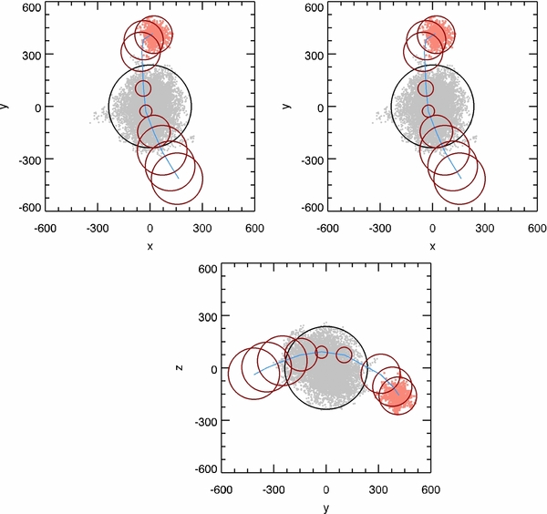
Figure 2. 5:1 flyby between an MW type halo and a satellite halo. The flyby starts at z = 1.1 and lasts until z = 0.3, for a duration of 4.7 Gyr. The gray and red points show the particle distribution of the FOF and the subhalo. The black and the dark red circles show the virial radius of the main halo and the subhalo throughout the encounter while the blue line shows the trajectory of the subhalo center of mass. This figure also shows the artificial mass-loss experienced by subhalos as they pass close to the main halo center.
Download figure:
Standard image High-resolution image4. RESULTS
4.1. Mass and Time Resolution Effects
In this section, we estimate the effect of particle resolution and snapshot timing resolution on the flyby rate. We have used a 5123 simulation and a 10243 simulation that is exactly the same phase for the results in this section.
In order to determine the sensitivity of flyby rates to numerical resolution, we conducted two experiments that degraded our fiducial simulation. In the first experiment, we explored the effect of particle number on the frequency of flybys with a 5123 simulation that was seeded with precisely the same initial random phases as the 10243 run (R. Scoccimarro 2011, private communication). Figure 3 centers on a typical MW halo in the volume—this halo experienced no difference in the number of mergers or flybys over its entire history. In the entire volume, the difference between the number of flybys in the two simulations is less than 1%, when we consider the halos that are well resolved in both simulations (i.e., down to the minimum halo mass in the 5123 volume of M < 6.7 × 10¹⁰ M☉ h−1). In addition, the number of flybys in two-dimensional mass and redshift bins are identical within Poisson error for 95% of the bins for these two simulations. So we find that particle resolution does not affect flyby rates.
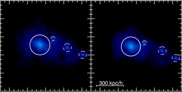
Figure 3. Solid white circle marks the virial radius of a typical halo extracted from the 5123 simulation (left) and the 10243 simulation (right) at z ∼ 1.8. Dashed white circles locate the other FOFs in the volume. Identical cubes of side 1 Mpc h−1 were extracted from both the simulations and projected to make this plot. This halo experienced the same number of merger and flybys throughout the run.
Download figure:
Standard image High-resolution imageThe second series of tests concerned the timing resolution of the simulation. In the 5123 simulation, we wrote snapshots in equal increments of log a, but never allowed more than 200 Myr between snapshots—this upper limit ensures that encounters for MW mass objects were resolved over the course of the run. With 161 snapshots, we made two new halo interaction network by skipping one and two snapshots, respectively. Thus, we have three samples built from 161, 80, and 54 snapshots, respectively, to quantify the effects of snapshot timing resolution on the flyby rate. We analyze these three samples and compare the total number of flybys between halos. We find that to get convergence in the flyby rate, the snapshot outputs need to resolve the "typical" flyby duration. Since a flyby is tagged as a main halo → subhalo → main halo transition, and we require flybys to last at least half a crossing time, the snapshots must be able to resolve events on timescales of ∼tcrossing. For the simulations with 161 and 80 snapshots, the crossing time was always resolved by snapshots and the resulting number of flybys differ by less than 1% and are within Poisson errors. However, the 54 snapshot simulation did not resolve the crossing time for most redshifts, and as a result the number of flybys is ∼20% lower.
As another test, we re-simulated the volume between z = 3 and 2 with a snapshot timing resolution of 25 Myr, which yielded 45 snapshots. The crossing times at z = 3 is ∼330 Myr, so it is very well resolved in this simulations. We take a similar approach as above, creating a series of progressively coarser halo interaction networks by skipping over snapshots. As before, we find that the number of flybys is consistent within Poisson error when we resolve the crossing time, and drops dramatically for coarser simulations. Thus, our definition of flybys produces consistent flyby rates as long as the snapshot outputs can resolve the crossing time. Otherwise, the flyby rates reduce as the time resolution degrades. This implies that simulations with insufficient outputs will underestimate the true flyby rate. Assuming that the time between snapshots is at most a quarter of the crossing time (such that flybys last for at least two snapshots), we find that the total number of snapshots required between redshifts 20 and 0 to be ∼132. This is in agreement with recent findings that show at least 128 snapshots are required to obtain a robust estimate of halo masses (Benson et al. 2012).
4.2. Frequency of Flybys
Now that we have a way to track and classify interactions between halos, it is useful to determine how common close flyby encounters are compared to mergers. This is an important first step in determining whether current semi-analytic and high-resolution N-body models could be missing a significant number of galaxy-transforming interactions. Note that in this census, we are simply keeping a tally of dark matter halo mergers and close halo flybys, regardless of how much they may perturb the potential of any galaxy embedded within. In the next paper, we will concentrate on quantifying the perturbation caused by these types of encounters. We checked to see if there are multiple flybys between the same halo pairs and found that ∼70% of the flybys do not recur. About 20% of flybys eventually become a merger, ∼6% are repeat flybys. Thus, flybys primarily represent one-off events between two halos.
In Figure 4, we present the number of flybys and mergers per Gyr per cubic Mpc as a function of redshift. Mergers dominate the overall rate of interactions for 12 ≲ z ≲ 4 by about an order of magnitude. However, at z ∼ 14, we see tentative evidence of an increase in the relative number of flybys compared to mergers. At low redshift, z ≲ 3, flybys start to become more prevalent. The impact of this on observed merger rate estimates may be profound: in large-scale surveys, the rate of close-pair galaxies is often taken as a proxy for merger rate, but if we assume that 50% of these halo flybys appear as galaxy flybys, then Figure 4 implies that at z ≲ 3, such galaxy-pair counts are going to be contaminated by flyby-halos at least at a 20%–30% level. Flybys also result in bimodal kinematic galaxy distribution near the virial radius, in that some galaxies are infalling for the first time, while other galaxies that were once much deeper inside the cluster potential are now leaving. Conceptually, these flyby galaxies are similar to "backsplash galaxies" (e.g., Gill et al. 2005; Moore et al. 2004; Knebe et al. 2011b).
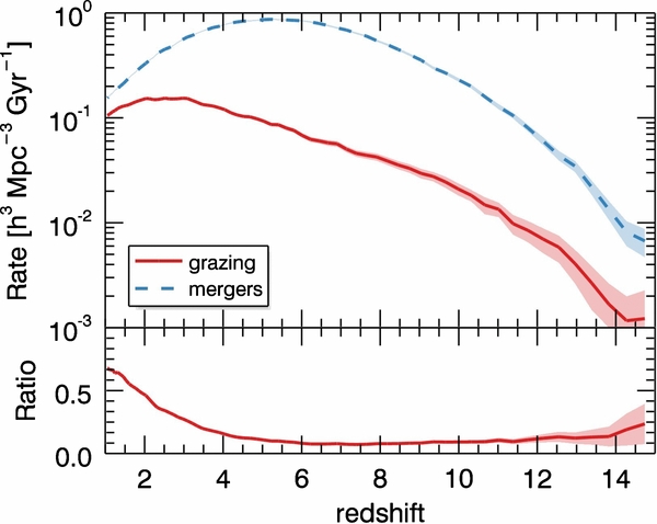
Figure 4. Top panel shows the number of mergers (blue, dashed line) and flybys (red, solid line) per comoving Mpc3 per Gyr as a function of redshift. The shaded region shows the Poisson error on the number of interactions. The bottom panel shows the ratio between the number of flybys to mergers vs. redshift. Mergers dominate flybys in the redshift range ∼4–12, but flybys become relatively more common at z ≲ 3. We can also see tentative evidence for an increase in the relative fraction of flybys compared to mergers at z ≳ 14. However, this increase is also due to the low number of interactions and is borne out by the large Poisson error at those high redshifts.
Download figure:
Standard image High-resolution imageWhile Figure 4 shows the global flyby rate, we need to know the rate of interactions as a function of both halo mass and redshift to assess the impact flybys may have on halo evolution. Interaction rates can be expressed either as "per object" or "per volume." Here, we plot the rates per halo to reduce the additional dependence of the halo mass function evolution. In Figure 5, we show the number of flybys and mergers on a per halo per Gyr basis, while the ratio of flybys to mergers is seen in Figure 6. We see that flybys are more frequent for higher-mass halos at all redshifts, consistent with the ΛCDM framework. From Figure 6, we can directly see that the number of flybys becomes comparable or larger than the number of mergers for halos >1011 M☉ h−1 for z ≲ 2. Such halos are expected to host galaxies—and the effect of flybys should leave an imprint on the observable properties. We also find tentative evidence that flybys are comparable in number to mergers at the highest redshifts, z ≳ 14; however, the numbers are affected by Poisson error and we can not conclusively say that flybys dominate mergers at those highest redshifts. We are simulating a bigger box size to look at the relative importance of flybys for z ≳ 14.
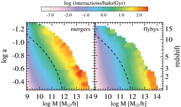
Figure 5. Number of mergers (left) and flybys (right) per halo per Gyr as a function of primary halo mass and redshift. The dashed line shows the mass accretion history of a typical MW type obtained from our simulations (Wechsler et al. 2002). The number of flybys increases with the primary halo mass for all redshifts, consistent with ΛCDM. For z ≲ 3, halos above 1012 M☉ h−1 have flyby rates greater than 100 per Gyr. Such a high flyby rate (in addition to mergers) means these halos are unlikely to be in equilibrium.
Download figure:
Standard image High-resolution image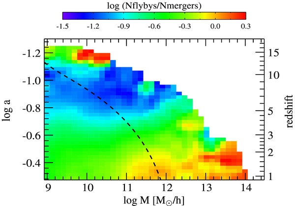
Figure 6. Ratio of the number of flybys to mergers as a function of primary halo mass and redshift. As we saw in Figure 4, mergers dominate flybys by an order of magnitude for 12 ≲ z ≲ 4. At lower redshifts, however, flybys start becoming more prevalent and by z ∼ 2, flybys are at comparable or even larger for all halos above 1011 M☉ h−1.
Download figure:
Standard image High-resolution imageIn the preceding mergers versus flybys comparison figures, we used all interactions irrespective of mass ratio, q. Now, it is interesting to see how the frequency of interactions compare as a function of both z and q for a typical MW halo. We select MW halos at z = 0 using three criteria: (1) the halo mass between 1 and 2 × 10¹² M☉ h−1, (2) the halo has always been a primary halo, and (3) the main progenitor of the halo can be traced back to z > 6. We found 178 such halos in our simulation box. In Figure 7, we show the average frequency of interactions per Gyr for these halos as a function of q and z. Mergers are dominant for 12 ≲ z ≲ 2 for all q; however, flybys take over for lower z. For these MW type halos, flybys and mergers happen with a similar frequency for z ≲ 2—a trend that we saw in Figure 6.
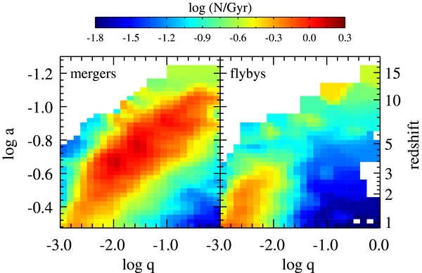
Figure 7. Average number of interactions per Gyr for an MW type halo (selected at z = 0) as a function of mass ratio (q) and redshift. Mergers are plotted on the left panel while flybys are on the right panel. As seen in the previous plots, mergers dominate flybys for all q values in the redshift range 12–2 but at flybys become comparable in number at lower redshifts.
Download figure:
Standard image High-resolution image4.3. Fits to Interaction Rates
Merger rates are usually calculated in two different ways: as a rate (1) per parent halo (2) per child halo. These two rates physically mean slightly different things—the first one is tied to the probability of a halo of a given mass at some z having a merger. Observationally, this is measured by the merger fraction through pair counts. The second one is the probability that a halo had a merger in the past—observationally identified by morphological features. Since we track subhalos, we can distinguish between the beginning of a merger (i.e., a main halo → subhalo transition; tied to the merger rate per parent halo) and the end of a merger (subhalo → main halo; tied to the merger rate per child halo). These two methods of measuring the merger rate can yield somewhat different results (see Hopkins et al. 2010). In this section, we will use the time of primary → subhalo transition as a merger time for the primary halo.
To compare to merger rates found in the literature, we use the analytic fit of Wetzel et al. (2009) and classify interactions per halo per Gyr in the form:
where, nevents is the number of mergers or flybys for a parent halo in some mass bin, nhalo is the number of halos in the same mass range, and dt is the time interval (in Gyr) between consecutive snapshots. We consider three different mass ranges for the parent halos, 1010–1011, 1011–1012, and 1012–1013 M☉ h−1. We limit the redshift range from z = 6 to 1.0. The fits for mergers and flybys are presented in Table 1. Overall, the values of A for flybys and mergers are comparable, while α is higher for mergers. Correspondingly, the flyby rate increases more slowly than the merger rate with increasing z.
Table 1. Fits to Equation (1) for Three Main Halo Mass Ranges
| M☉ | 1010–1011 | 1011–1012 | 1012–1013 | |
|---|---|---|---|---|
| Mergers | A | 1.33 × 10⁻³ | 1.61 × 10⁻² | 3.84 × 10⁻¹ |
| α | 2.40 | 2.58 | 1.16 | |
| χ2 | 10.6 | 3.05 | 1.45 | |
| Flybys | A | 1.08 × 10⁻³ | 1.92 × 10⁻² | 2.59 × 10⁻¹ |
| α | 1.02 | 0.75 | 0.68 | |
| χ2 | 2.33 | 1.63 | 0.88 | |
Notes. The redshift is noted when the subhalo first appears inside the main halo. The reduced χ-squared values for the fits are also shown in the table.
Download table as: ASCIITypeset image
5. DISCUSSION
We present a technique for tracking the dynamical history of halos in an N-body simulation. Since many of these interactions are close flybys and not mergers, we call this ensemble the halo interaction network. We find that most of the anomalies common to merger-tree construction arise from limitations in the halo finding algorithm, and we correct for those in creating the halo interaction network. For example, density contrast based methods like SUBFIND are unable to track a subhalo when it reaches a denser central region. In most cases, such close pericenter passages manifest as severe mass loss in the subhalo (with a fraction of the mass regained when the subhalo is farther away from the host center), and at times, the entire subhalo falls below the minimum particle limit and is not identified at all. There are also issues of nomenclature: in a near equal-mass major merger, it is unclear which halo is the dominant one, i.e., which halo is to be labeled the "main" halo. The algorithm we have presented here tracks several pathological cases and corrects them. We find that even after fixing all such cases, there still remain halos that are parentless or childless at a few 10% level for halos comprised of ≲80 particles. Even with very finely spaced snapshot outputs, we can not eliminate all of these ill-behaved halos. Based on our findings, we recommend that semi-analytic studies based on N-body merger trees use only those halos with at least three to four times the formal particle limit. In our simulations, we formally require 20 particles to identify a halo, but all the results that have been reported here involve halos with at least 100 particles.
For robust halos, our merger-tree technique resolves anomalies related to halo definition and problems with halo identification; however, the code can still be improved using maximal bipartite graph matching (e.g., Hopcroft & Richard 1973). Given two sets of halos at two different snapshots and an associated cost (say, the inverse of the binding energy rank) for matching any two of them, the maximal matching algorithms can be used to determine a match. Such a technique would produce the least number of anomalies and spurious initial assignments in a merger tree, and we will implement it in a future version of the merger-tree code.
One major thrust of this paper is to include flyby interactions in our halo interaction network. In this paper, we present the first census of halo flybys across a wide range of halo mass and redshift. We classify a flyby using spatial and dynamical information. Conceptually, a grazing flyby occurs when a halo undergoes the transition from a main halo → subhalo → a main halo and is fundamentally different from mergers. In a simulation, it is relatively straightforward to identify such chains since the current kinematics and future behavior of a given interaction is fully determined. We note that because flybys imply a population of galaxies that were once well within the virial radius of the main halo but are now outside it, they may be related to so called "backsplash" galaxies. The morphological and kinematical features of these galaxies are likely to be different compared to other galaxies that are infalling for the first time (Gill et al. 2005; Moore et al. 2004; Knebe et al. 2011b). In some cases, these flybys can even result in subhalos switching their main halo and appear as "renegade" subhalos (Knebe et al. 2011a). While there has been a significant amount of work related to "backsplash" galaxies in clusters (e.g., Balogh et al. 2000; Sanchis et al. 2002; Gill et al. 2005; Moore et al. 2004; Mamon et al. 2004; Knebe et al. 2011b; Mahajan et al. 2011), unfortunately there are no systematic studies for lower-mass halos.
We suspect flyby interactions have been unappreciated in both observational and theoretical studies that attribute morphological/structural changes to mergers. For example, the pre-dominance of low-mass bulge-dominated galaxies (Mstellar ∼ 1010 M☉ h−1) may be potentially explained by perturbations caused by flybys, since low-mass galaxies do not suffer enough mergers to explain the bulges (Weinzirl et al. 2009). Indeed, flybys can cause a fractional change in the binding energy of the primary halo, ΔE/E > 1%—this may excite bars (see Berentzen et al. 2004 and references therein) and drive gas into the central regions of the galaxy, creating a pseudo-bulge. Observationally, barred and unbarred galaxies can not be separated on some inherent galaxy property (other than the actual presence/absence of a bar); this implies that the formation or destruction of a bar is likely linked with some external process, such as a flyby (Sellwood 2010). In addition to forming bars/pseudo-bulges, flybys could create density enhancements via shocks in the hot halo gas of the primary galaxy. Such density enhancements will increase the cooling rates in the halo by ∼ an order of magnitude (assuming bremsstrahlung and a factor of four, increase in density). In principle, this can cause the hot gas to cool and replenish the disk (Sinha & Holley-Bockelmann 2009). In a similar spirit, flyby-induced star formation has been recently invoked to explain the steepness of the [α/Fe]–σ relation (Calura & Menci 2011). Flybys can also cause various other morphological features or transformations, e.g., spiral to S0 galaxy in groups (Bekki & Couch 2011), spin flips in the inner halo (Bett & Frenk 2012), or spiral arms in the galactic disk (e.g., Tutukov & Fedorova 2006).
6. CONCLUSIONS
In this paper, we report on a new class of interactions—flybys, that occur frequently. Most of these flybys are one-off events—one halo delves within the virial radius of another main halo, separates at a later time and does not return. From our testbed simulation, we can see a hint that flybys dominate over mergers at very high redshift (z ∼ 14) and have a relatively shallower dependence on z compared to mergers (see Table 1). We find that most flybys are one-off events and about 70% of the flybys do not ever return. Flybys are then a largely ignored type of interaction that can potentially transform galaxies. Unfortunately, most semi-analytic methods of galaxy formation are designed only to use mergers, and thus can not account for the effects of flybys directly. In principle, a flyby can create long-lasting features to appear in the secondary halo and affect the evolution of that halo. In general, slow flybys cause a larger perturbation compared to a fast one, and such features can persist even when the perturbing halo has moved far away (Vesperini & Weinberg 2000). If flybys cause perceptible changes in galactic structure, then those deviations should manifest in the oldest galaxies. Upcoming space telescopes like James Webb Space Telescope will target high-redshift (z ∼ 7) galaxies to unravel clues for galaxy formation and may be able to detect flyby signatures.
In conducting our flyby census, our testbed simulation did not have adequate resolution to capture the perturbative effect of a flyby on the dynamics of the halo central region. We are currently exploring the effect of flyby interactions on galaxy structure and morphology using both high-resolution N-body simulations and semi-analytic estimates (M. Sinha & K. Holley-Bockelmann, in preparation).
This work was conducted in part using the resources of the Advanced Computing Center for Research and Education at Vanderbilt University, Nashville, TN. We also acknowledge support from the NSF Career award AST-0847696. Some of the simulations were run on the Pleiades cluster at NASA Advanced Supercomputing Division. We thank the anonymous referee for helpful comments. M.S. thanks Frazer Pearce and the organizers of the workshop "Haloes Going MAD" for motivating some sections in this paper. M.S. also thanks H.R. Madhusudan for pointing out bipartite graph matching algorithms.
APPENDIX: HALO GENEALOGY: FINDING PROPER PARENT–CHILDREN PAIRS
Our first step is to track the main halos through time. Since even simple isolated halos change mass and position in each snapshot, this is not a trivial task. Overall, we link main halos and subhalos with different techniques. In most cases, we can assign the proper parent for a main halo in the following ways.
- 1.Gather all the particles in all main halos at two consecutive snapshots. Note that this includes the particles in the subhalos because some of these particles may have joined (or left) the main halo between these two redshifts.
- 2.Working backward from a later snapshot, we compare the particle IDs in one halo with the IDs in all primary halos at the previous snapshot. For computational efficiency, once a particle ID is matched across two snapshots, we store the actual subhalos at the particle level.
- 3.Assign the parent3 halo as the one with the largest number of common particles.
- 4.Repeat for all remaining primary halos at the later snapshot.
- 5.If several child halos claim the same parent (i.e., the parent halo may have split apart), then the parent is assigned to the most massive child halo. In other words, a parent may have at most one child halo in our scheme. In addition, one child halo can have at most one parent at this stage—though this may change at the subhalo matching step.
Using this procedure, we assign ∼90% of the main halos to a parent. If the halo is still unassigned, then we treat it as though it were a subhalo. Subhalos are matched using a binding energy technique described below.
In the SUBFIND algorithm, a subhalo is a self-bound group of particles. Therefore, an acceptable parent–child pair should have most of the highly bound particles in common. We track the subhalo core (similar to Okamoto & Habe 2000; Springel et al. 2005c; De Lucia & Blaizot 2007; Boylan-Kolchin et al. 2009) using a binding energy rank similar to Boylan-Kolchin et al. (2009). For every particle that is common between two halos, we compute the quality,  , as
, as
where "prev" and "next" refer to the halo at the previous and later snapshot, and  is the binding energy rank (1 for the most bound, 2 for the next, and so on) of the common particle; this choice weights the core of a halo more strongly than the outer regions. We limit the number of particles in
  to 100, because in cases of severe tidal stripping, only the core remains—the rest of the subhalo is spread to the main halo background. If no child subhalo is found, then we search two later snapshots using this binding energy rank method. This yields a parent–child match for over 99% of the halos.
After the parent–child matching is done for all halos and subhalos, we manually check the assignments for validity and make adjustments if necessary. We found that the parent–child pair misassignments typically fell into two classes—those caused by major mergers, and those caused by numerical resolution. Major mergers caused <1% of the misassignments while particle resolution resulted in the remainder of the poor parent–child pairs. During a major merger, the process may be so violent that a large parent subhalo is the only thing that survives relatively intact, while the main parent halo is mixed throughout the remnant. In this case, the parent halo and subhalo effectively "swap" categories after the merger. However, because our halo matching takes place before subhalo matching, our algorithm inaccurately assigns both the parent halo and the subhalo to the same main child halo after the merger. The consequence of this is that it eliminates an entire branch of the merger tree. To correct the pairing, we search for this pattern in the parent–halo pairs, demote the main parent halo to a child subhalo, and reinstate the missing branch.
A.1. Tracking the Network of Interactions
The parent-finding step described in the previous section simply links one halo to another between two time steps, where possible. To make the halo interaction network, we must both uniquely track every halo from its formation to its destruction (or to the present day if it survives) and categorize every dynamical interaction between two or more halos. The procedure for tracking the halo is quite similar to our technique for pairing an individual parent and child halo, and amounts to constructing a merger tree; for completeness sake, however, we describe how we follow a halo through its lifespan. First, for every child halo at a given snapshot, we identify all the parents that comprise the child: these parent halos are all direct parents, but may each have joined the child halo at different redshifts. We choose the most massive parent as the primary halo, and assign unique halo IDs that are preserved as we step backward in time along a particular halo branch.
While the halo-pairing step addressed most anomalies, there is one anomaly that can only be addressed during this step: when a subhalo passes through a dense region of the halo, it seems to disappear because SUBFIND cannot differentiate it from the background halo. This means that when the subhalo reappears several snapshots later, it will seem brand new. To graft these apparently new subhalo branches to their proper place in the network, we first locate all the subhalos that do not have parents, and search among all subhalos up to five snapshots earlier for a suitable parent based on particle IDs. A potential match contains more than 50% of the particles of the orphaned subhalo and is not a primary parent of any other halo. Once the parent subhalo match is found, we attach the apparently orphaned subhalo branch to this parent subhalo (see Figure 8 for a schematic).

Figure 8. Schematic for finding the parents of subhalos passing through a dense halo center. Time increases vertically downward. As the subhalo passes through the central region, the density contrast becomes too low for SUBFIND to identify it; consequently, original particles from the subhalo blend with the halo background. At some later snapshot, when the subhalo is sufficiently far from the center, SUBFIND identifies it as a subhalo (left). Left alone, the parent-matching algorithm will lose the subhalo in step 1 to the main halo in step 2, and mistakenly identify a new parentless subhalo in step 3. We remedy this by checking that the subhalo in step 3 can be found in the same halo in an earlier snapshot.
Download figure:
Standard image High-resolution imageThese orphans occur in a very small mass range. So, fixing them does not dramatically increase the overall 99% successful of parent–child assignments. The anomalies described in Tweed et al. (2009) are also present in our technique.
- 1.No child. None of the halo particles were found in any other halo, up to three snapshots into the future.
- 2.No parent. Either none of the halo particles were found in another halo up to five snapshots in the past, or the potential parent halo has already been matched with a child halo.
- 3.Transients. The halo appears to be a transient phenomenon—none of the halo particles are present in any future or past halo. We determined this to be largely an effect of numerical noise, as we will discuss in the next section.
A.2. Halo Tracking and Particle Number
In Figure 9, we show the cumulative distribution, over all snapshots, for the total number of parentless, childless, and transient halos versus halo mass. To generate the plot, we bin in mass for all the snapshots in a specified redshift range and count the total number of halos that are either parentless or childless. This is divided by the total number of halos in the same range to give a fractional occurrence of the anomalies.
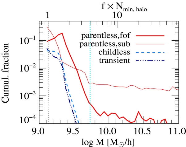
Figure 9. Cumulative fraction of halo anomalies as a function of halo mass. The different lines represent parentless halo (thick solid), parentless subhalos (thin solid), childless (dashed), and transient (dash-dotted). The number of childless and transient halos drops off very sharply with mass, suggesting that both are caused by numerical noise. The parentless halos show a peak near our halo detection threshold—these are all the newly formed halos and hence do not have a parent. The parentless subhalos show a very gradual decline with mass, and can be interpreted as a combination of two effects: (1) timing resolution—a new halo forms and is accreted by another halo to become a subhalo between two snapshots (2) a subhalo splits into two. The upper X-axis shows the number of resolution elements in a given halo mass; the cyan dotted line shows our recommended minimum halo particle threshold to limit transient behavior at or below the 1% level for reasonable timing resolution. The black dotted line shows the halo detection limit (20 particles), while the cyan line is four times that value.
Download figure:
Standard image High-resolution imageIt is clear that the number of childless and transient halos drops off very rapidly with particle number, and is essentially zero for halos resolved with ≳ 80 particles, or about four times our nominal halo detection threshold. This implies that the typical particle number threshold (∼20 particles) for resolving halos is much too small to produce robust results. A different halo finder and merger-tree technique has found similar results (D. Tweed 2010, private communication). With these results in mind, we find that a halo is unlikely to be noise once it is above ∼4 times the canonical particle number threshold for halo detection. For the science results in the paper we will employ an even more conservative limit of 100 particles per halo, five times our halo detection threshold.
A.3. Halo Tracking and Time Resolution
Both parentless halos and parentless subhalos can occur; we expect most of the parentless halos to be legitimate, newly formed halos. However, some of the parentless subhalos may actually be caused by a newly formed halo that is quickly accreted by another primary halo in between two snapshot outputs. To test this hypothesis, we increased the output resolution of the simulation by an order of magnitude between z = 6 and 5, resulting in a snapshot every few time steps.
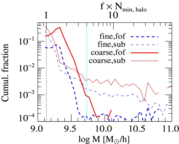
Figure 10 shows the percentage of halos that are parentless/childless in the redshift range z = 6–5 for two simulations with differing snapshot output resolution. Our fiducial simulation, which we label as "coarse" in this plot, already has good timing resolution (see Section 2) but still produces anomalies at the ∼5%–10% level in the low-mass halos. The "fine" simulation increases the snapshot output by a factor of 10 which reduces the level of anomalies by a factor of 2–3 over the entire mass range. Figure 10 shows that the overall number of parentless subhalos dropped with this increased output frequency, though never to the level of parentless halos. The slope for parentless subhalos are similar in the two simulations; in fact, we note that the overall shape of the parentless subhalos mimics the cumulative mass function, albeit with a much lower amplitude. We expect that increasing the time resolution even further will reduce the amplitude, but a fraction of parentless subhalos will still remain. In the "fine" simulation, the fraction of parentless subhalos reduces to the ∼1% at only twice the halo detection limit, but such accuracy in the halo interaction network comes at the price of disk output—a full-scale cosmological simulation would need ∼2000 snapshots (assuming log a output spacing) to achieve the timing resolution of the "fine" simulation. The number of childless/transient halos is indistinguishable between the two simulations—showing that they are indeed dominated by numerical noise.
Figure 10. Dependence of parentless halos for the z range 6–5, as a function of time resolution of snapshots. The red line shows our fiducial simulation while the blue shows the a re-simulation with 10 times as many snapshots. The number of parentless halos in the fine simulation reduces by factors of 4–5 compared to the coarse one. While the number of parentless subhalos is also reduced in the fine simulation, the drop is smaller. With such a high time resolution, we can reduce the fraction of parentless (sub)halos to the few % level for halos that are only twice the detection limit. To achieve the fine time resolution shown here, a simulation would have to output about 2000 snapshots for z = 20 to 0 (assuming steps in log a). The transients/childless halos show virtually no difference between the two simulations and have been omitted from the plot.
Download figure:
Standard image High-resolution image
A.4. Comparison of our Technique to Previous Numerical Work
A merger tree simply identifies the links between components of a halo across redshifts. For particle-based codes, this means tracking halo particles by particle ID across various snapshots. Nevertheless, the complexity of halo histories makes the task non-trivial. As we noted earlier, most halo finders use some form of a density contrast (e.g., Springel et al. 2001a; Knollmann & Knebe 2009; Klypin et al. 1999) to group particles into a subhalo (see VOBOZ, Neyrinck et al. 2005; EnLink, Sharma & Johnston 2009; HSF, Maciejewski et al. 2009; and Rockstar, Behroozi et al. 2011, for different approaches). Such a technique fails to identify subhalos close to the center of the host halo. Hence, it is important to isolate such cases and reassign the subhalos that "disappear." In this section, we compare the various strategies that have been employed to construct a merger tree based on subhalos identified in N-body simulations. In particular, we compare our merger-tree methods to those in Wechsler et al. (2002), Wetzel et al. (2009), Boylan-Kolchin et al. (2009), and Tweed et al. (2009).
In Wechsler et al. (2002), a parent–child halo was assigned such that more than 50% of the particles in the parent end up in the child along with those 50% of particles constituting more than 70% of the particles in the parent that end up in any halo. This technique is also labeled as the "most massive progenitor" method. Such an algorithm is prone to misassignment of parent–child halos in cases where a subhalo undergoes massive stripping or completely disappears inside a host halo.
In Wetzel et al. (2009), the authors use the 20 most bound particles of a subhalo (that also occur in the potential child) to construct a parent–child pair. They compute the potential of these common particles based on all the particles in the parent and weight against large increases in mass or scale factor. However, the weighting function is linear in mass (Equation (2)) while the potential itself is squared (Equation (1)). If a subhalo appears to have dissolved into the host halo, then the large potential term could outweigh the limiting weighting function. As such, it is not obvious that this formulation would always pick the "right" subhalo as a child. In addition, since N-body simulations have discrete outputs, weighting by the ratio of the scale factors of the parent–child pair could change depending on the output frequency of the same simulation.
Tweed et al. (2009) specifically made the merger tree to account for the cases we have discussed in this paper. They assign parent–child pairs by choosing the halo pairs with the maximum common mass as the main parent. In addition, they identify (and remedy, if possible) three classes of anomalies: (1) subhalos without a parent, (2) subhalo that becomes the parent of a primary halo, and (3) subhalo and host halo swap identities. As we mentioned, we find two of these cases in our technique: anomaly 1 occurs under two circumstances—when the time resolution of the outputs is too coarse or when the subhalo appeared to have "dissolved" in the host halo at some earlier snapshot. We correct for the dissolved halos in our interaction network. Anomaly 2 does not appear in our simulations since we first match main halos across two snapshots before matching subhalos. An analog of anomaly 3 occurs in our technique for major mergers—when SUBFIND switches the main halo and dominant subhalo definition across two snapshots. We have outlined our method to fix these cases in Appendix A.1. Overall, the approach described here and those used by Tweed et al. (2009) agree qualitatively. We reiterate the cautionary statement from Tweed et al. (2009) that careful analysis has to be done to grow an "accurate" merger tree. Although the anomalies that we have described and fixed represent ≲ 5% of all halos, it is not clear to us what the cumulative effects of such anomalies are on semi-analytic approaches.
Specifically, the advantages in our merger-tree technique are as follows.
First, it uses different strategies to locate descendants for main halos and subhalos. Descendants of main halos are assigned based on the highest number of common particles, subhalo descendants are assigned according to the binding energy rank (see Equation (A1)). The rank computation is symmetric, i.e., a highly bound common particle always adds to the total rank. Using only common particles or binding energy rank leads to misassignments, e.g., a highly stripped subhalo will be lost even when the core survives or a main halo will get assigned to a subhalo that happens to contain some of the most highly bound particles from the previous step.
Second, it carefully corrects the following pathological cases to the 0.1% level:
- 1.a subhalo and main halo switching definition across time steps;
- 2.a subhalo appearing to dissolve into the main halo due to massive tidal stripping (even though the core of the subhalo survives);
- 3.when a subhalo (including the core) seems to disappear for multiple snapshots while passing close to the center of a main halo.
Footnotes
- 1
A particle is associated with only one subhalo.
- 2
We used the total mass of the main halo, including all the subhalos, as proxy for the virial mass, and assumed a spherical halo to get the virial radius.
- 3
Here a parent halo lies in the past. Note that Extended Press–Schechter usually has the opposite convention.