


ABSTRACT
We introduce a probabilistic approach to the problem of counting dwarf satellites around host galaxies in databases with limited redshift information. This technique is used to investigate the occurrence of satellites with luminosities similar to the Magellanic Clouds around hosts with properties similar to the Milky Way (MW) in the object catalog of the Sloan Digital Sky Survey (SDSS). Our analysis uses data from SDSS Data Release 7, selecting candidate MW-like hosts from the spectroscopic catalog and candidate analogs of the Magellanic Clouds from the photometric catalog. Our principal result is the probability for an MW-like galaxy to host Nsat close satellites with luminosities similar to the Magellanic Clouds. We find that 81% of galaxies like the MW have no such satellites within a radius of 150 kpc, 11% have one, and only 3.5% of hosts have two. The probabilities are robust to changes in host and satellite selection criteria, background-estimation technique, and survey depth. These results demonstrate that the MW has significantly more satellites than a typical galaxy of its luminosity; this fact is useful for understanding the larger cosmological context of our home galaxy.
Export citation and abstract BibTeX RIS
1. INTRODUCTION
Our home galaxy, the Milky Way (MW), is in many respects the best-studied galaxy in the universe. There are numerous measurements that can only be made in the MW, including detailed studies of resolved stellar populations and the detection and dynamical measurements of the faintest satellite galaxies. Furthermore, the MW is a critical testbed for dark matter studies, as it is one of the only places where self-annihilation or weak interactions can be directly observed. As such, studies of the MW have long provided key insights into aspects of cosmology and galaxy formation.
To fully interpret this panoply of observations of the MW in the context of a cosmological model, it is essential to understand whether or not the MW is a typical galaxy of its mass or luminosity. One of the most cosmologically interesting statistical properties of the MW that can be readily studied is the number and properties of its satellites. It has been apparent for more than a decade that N-body simulations of Galaxy-sized (i.e., M ∼1012 M☉) dark matter halos predict an abundance of low-mass subhalos that exceeds the observed population of MW dwarf satellites by more than an order of magnitude (Moore et al. 1999; Klypin et al. 1999b; for recent reviews, see Bullock 2010; Kravtsov 2010); this is the so-called missing satellites problem. A number of different theoretical solutions to this problem have been proposed, focusing either on reducing the small-scale power in the dark matter power spectrum, or on suppressing galaxy formation in low-mass halos (see, e.g., Madau et al. 2008; Busha et al. 2010 and references therein).
In the last several years, it has become apparent that some of this discrepancy was due to galaxies that had not yet been observed. The unprecedented deep, wide-field imaging from the Sloan Digital Sky Survey (SDSS; York et al. 2000) has yielded detections of a substantial number of previously unknown dwarf companions to the MW (e.g., Belokurov et al. 2007; Walsh et al. 2009). This has led to a reassessment of the missing satellites problem from the observational side, with the result that proper accounting for the detectability of MW dwarf satellites (Koposov et al. 2008) results in substantial upward corrections to the satellite luminosity function. This leads to the prediction that the MW hosts hundreds of faint satellites that are currently undetected (Tollerud et al. 2008; Walsh et al. 2009).
By contrast, there has been some indication that the missing-satellites problem might reverse itself at high masses: high-resolution Galactic-halo simulations generally have too few subhalos in the mass range of the Large and Small Magellanic Clouds (LMC and SMC; e.g., Madau et al. 2008). However, it has been difficult to draw robust conclusions on this point, since the numbers of high-mass subhalos, such as those that might host the Magellanic Clouds, are few in number for any individual Galactic-halo simulation, and in any case the abundance of such massive subhalos might be suppressed by the limited number of long-wavelength density-fluctuation modes in a small simulation volume.
With the completion of recent high-resolution N-body simulations over cosmological volumes, such as the Millennium II and Bolshoi simulations (Boylan-Kolchin et al. 2009; Klypin et al. 2010), it has become possible to probe analogs of the MW–LMC–SMC system with greatly improved statistical significance, since these simulations can resolve LMC- and SMC-mass subhalos in large numbers of MW-mass halos. For example, Boylan-Kolchin et al. (2010) found that MW-mass halos (with Mhalo ∼ 1012M☉) seldom host subhalos that can be identified as analogs to the Magellanic Clouds, with less than 10% of MW-sized halos hosting two such subhalos. Similar results are seen in the Bolshoi simulation, as will be discussed in a companion paper to this one (Busha et al. 2011b). It thus appears that the MW–LMC–SMC system is somewhat atypical in the context of the cold dark matter paradigm.
On its face, this theoretical result seems to be mildly anti-Copernican, so it is especially important to confront it with observational data. But any satellite-counting exercise is classically complicated by the faintness of the satellites, which makes obtaining redshift information difficult. Redshift-space studies of satellite dynamics that have aimed to probe galaxy halo masses (e.g., Zaritsky et al. 1993; Prada et al. 2003; Conroy et al. 2005, 2007) or profiles (e.g., Chen et al. 2006) have typically had redshift information for ≲ 1 satellite per host galaxy, even while using criteria for satellite selection that are significantly more relaxed than we would like to use to select LMC/SMC analogs. Indeed, as discussed in Section 2.4 below, even the vast SDSS spectroscopic database contains less than 100 MW-like systems that host one or more MC-like satellites with redshifts.
A common method for overcoming the lack of spectroscopic information for satellites has been to count candidate satellites around bright hosts in photometric data and to statistically subtract or correct for the contribution of foreground and background objects (hereafter, we will simply use the term "background" as a shorthand to refer to both foreground and background objects). In a pioneering paper, Holmberg (1969) found that nearby bright spiral galaxies, with a rather wide range of luminosities, typically hosted between 0 and 5 satellites brighter than an absolute magnitude around −10.6. Lorrimer et al. (1994) carried out a similar analysis and found that galaxies brighter than  host 1.1 satellites in the range
  , on average, with fewer satellites around spirals (0.5 on average) than ellipticals (1.8). Both of those studies accounted for background contamination by subtracting off the average number of faint galaxies in nearby fields from the counts around bright galaxies; therefore, they were only able to measure the average number of satellites around bright galaxies; as discussed in Section 3, they cannot address the probability of hosting a certain number of satellites, which is what we have set out to do here.
Recently, James & Ivory (2011) carried out a quasi-spectroscopic analysis by targeting 143 bright galaxies of known redshift for follow-up with narrow-band imaging centered near the expected wavelength of Hα at the redshift of the target galaxy. This allowed them to count the number of roughly MC-like star-forming objects within a few hundred km s−1 of each host, yielding a plausible measurement of the satellite number-count distribution. In broad agreement with simulations, they find that roughly two-thirds of their target galaxies have zero such satellites, while only ∼5% have two. This clearly confirms that the Magellanic Clouds are indeed quite rare. There is significant uncertainty in the details, however, owing both to the small sample size and to the width of the imaging band, which will detect galaxies in Hα up to 30 Mpc away from the host along the line of sight, so the potential for significant background contamination remains.4 In addition, comparison to the subhalo population in simulations is difficult, since only star-forming galaxies are selected.
In this paper, we employ the enormous statistical power of the SDSS to obtain a statistically robust result for the frequency of LMC and SMC analogs in galaxies like the MW. We use the main SDSS spectroscopic catalog to identify a sample of >2 × 10⁵ isolated galaxies with luminosities similar to the MW. As in the studies above, we then count photometric companions around host galaxies with known redshifts, but here we introduce a new technique for statistical background removal that allows us to recover the true probability distribution of satellite number counts around these hosts, P(Nsat). To do this, we make use of the fact that our measured number counts represent a convolution of the true satellite distribution with the distribution of background counts. We can also measure the latter distribution in the data, and then a simple deconvolution yields the desired result. We pay careful attention to the details of our background-estimation techniques to ensure that we account for all possible sources of systematic error, particularly those arising from the clustering of background galaxies with our hosts.
Our principal result is that only 3.5% ± 1.4% of galaxies with luminosity similar to the MW host two satellites similar to the Magellanic Clouds within a radius of 150 kpc. When we split the sample into red and blue hosts, we find that excluding red-sequence galaxies from our sample of hosts has no significant effect on the probability of hosting any number of bright satellites. This confirms that the MW–LMC–SMC system is indeed quite unusual compared to the population of isolated galaxies with similar luminosity and color. These results are also broadly consistent with the predictions from simulations (Boylan-Kolchin et al. 2010). We present a detailed comparison with the predictions of high-resolution ΛCDM simulations in a companion paper (Busha et al. 2011b); the general conclusion from both simulations and observations is that the MW–LMC–SMC system is quite rare.
This paper is structured as follows. First, we describe the SDSS data set and our criteria for selecting analogs to the MW, LMC, and SMC in Section 2. In Section 2.4 we perform a preliminary analysis on SDSS galaxies with spectroscopically identified satellites. Finding it difficult to cleanly interpret these results, we then move on to develop our photometric background subtraction method in Section 3, being careful to fully account for the statistical and systematic error budget. We perform the counting and background-correction exercise in two different ways, which have different approaches to handling systematic errors. We obtain similar results for these two different procedures, which we present in Section 5. In that section, we also discuss the sensitivity of these results to a number of assumptions in the analysis. We also perform an additional analysis in the deep photometric data from SDSS Stripe 82 to test the robustness of our analysis. We discuss the implications of our results in Section 6.
Throughout, distances and absolute magnitudes are calculated using a flat ΛCDM cosmological model with Ωm = 0.3. All distances quoted in this paper are given in physical (rather than comoving) units, and all distances and absolute magnitudes derived from SDSS data assume a Hubble constant of H0 = 70 km s−1 Mpc−1.
2. DATA AND SAMPLE SELECTION
2.1. SDSS Catalogs
We use data from the spectroscopic and imaging catalogs of the SDSS seventh data release (DR7; Abazajian et al. 2009). Because our potential MW–LMC–SMC analogs are at very low redshift, and because we require them to be more than 500 kpc from a survey edge (see Section 2.2), this limits the area used for the analysis. The main sample of MW-sized hosts is selected from among the spectroscopic targets in a contiguous, 3350 deg2 section of the Northern Galactic Cap. The deeper imaging in Stripe 82 (an approximately 280 deg2 strip along the celestial equator) allows for a second, much smaller sample of MW analogs extending to slightly higher redshifts in the southern sky (we analyze this data separately to check the robustness of our methods; see Section 5.3.2). Spectra and k-corrected luminosity values are taken from the NYU Value Added Galaxy Catalog (NYU-VAGC; Blanton et al. 2005b).5
The r-band magnitude limit of the main (non-QSO) spectroscopic galaxy catalog is 17.77. We use this limit along with the PRIMTARGET type designation to isolate only those members of the main catalog identified as galaxies. We refer to the resulting catalog as the spectroscopic galaxy sample. Since we are interested in relatively faint satellites (between 2 and 4 mag dimmer than their hosts), the spectroscopic catalog alone is insufficient for our purposes. In order to collect ample statistics we must also use the SDSS photometric data, which is complete down to at least r ∼ 21.5 for extended sources.
Our general strategy is to select candidate MW-sized host galaxies from the spectroscopic sample and conduct our search for satellites around these objects within the deeper imaging catalog. From the NYU-VAGC we obtain the k-corrected absolute magnitudes for potential hosts computed using spectroscopic redshift information. From the imaging catalog, we obtain apparent magnitudes of galaxies and photometric redshift information. In our core analysis, we use photometric redshift probability distributions, p(z), determined by Cunha et al. (2009) for the DR7 SDSS imaging catalog using an artificial neural network algorithm.
2.2. Selection of Milky-Way-sized Central Galaxies
2.2.1. Luminosity Requirements
As discussed in Section 2.3, we count candidate LMC/SMC analogs by looking for galaxies 2–4 mag fainter than their hosts. Thus, we limit our pool of potential hosts to galaxies more than 4 mag brighter than the limit of our photometric sample. Objects dimmer than r = 21 in the imaging catalog are particularly prone to catastrophic photo-z failures, owing to their large photometric errors and the sparseness of the available spectroscopic training set. We therefore limit the pool of potential MW-analog hosts to apparent magnitude r < 17 to avoid this uncertain regime in the photometric sample (in the deeper co-added stripe 82 data we consider hosts as dim as r = 17.6). From this reduced spectroscopic sample, we select a statistically robust set of MW-luminosity hosts as follows.
The current best estimate for the absolute magnitude of the MW is MV = −20.9 in the Vega photometric system (van den Bergh 2000). In order to translate this value to the SDSS photometric system, we convert to the AB system and also apply an appropriate magnitude correction to the SDSS r filter (which is the filter that has the strongest overlap with V). To accomplish the latter conversion, we compute estimated absolute 0.0V and 0.1r-band magnitudes6 for a large sample of SDSS spectroscopic targets, using the kcorrect algorithm, version kcorrect v4_1_4 (Blanton & Roweis 2007). We then compute the mean V−r color for galaxies within ±0.2 mag of the MW and apply this average correction to the measured MV of the MW. Because the V and r bands overlap strongly, this correction is quite small (so, for example, splitting the sample by color before computing it will not make a significant difference). The resulting absolute 0.1r-band magnitude of the MW is M0.1, r = −21.2. We consider a galaxy to be a potential MW-like host if it is within ±0.2 mag of this absolute magnitude.
It is worth noting in passing that the absolute magnitude of the MW is difficult to measure and may be subject to quite large uncertainties. Since these are rather difficult to quantify, we adopt a best-guess value for the MW luminosity here and defer study of the satellite population's dependence on host luminosity to future work.
2.2.2. Isolation Criteria
Our aim is to count MC-like satellites around MW-like host galaxies. To ensure that the satellites we are counting are indeed hosted by MW analogs, we require that each candidate host, like the MW itself, is not itself a satellite of a more massive system.7 This criterion is simple to impose if we presume that there is a monotonic relation between dark matter halo mass and galaxy luminosity: we can then impose a radius of isolation (Riso), within which no other similarly luminous galaxy may reside. More specifically, a candidate host is eliminated if, within this region, (1) a galaxy brighter (in absolute magnitude) than Mhost + ΔMiso is found within ±1000 km s−1 of the host redshift, or (2) a galaxy brighter (in apparent magnitude) than mhost + ΔMiso is found with no redshift information.8 In our primary analysis, we set ΔMiso = 0 and reject only those candidate hosts with a brighter neighbor. In Section 5.3, we also consider the impact of a more stringent condition, requiring that our MW analogs have no close neighbors of similar brightness (up to ΔMiso = 2), and we show that the results are insensitive to this detail.
The exact choice of Riso naturally involves some trade-offs. The primary impact of varying Riso will be to change the purity and completeness of the sample of isolated hosts. Here, purity refers to the fraction of surviving MW analogs which are indeed isolated, that is, which are not satellites of more massive galaxies. Completeness is the fraction of truly isolated hosts that pass through our isolation filter. To explore the effect of the Riso parameter on these statistics, we consider its impact on dark matter halos identified in a cosmological N-body simulation.
Figure 1 shows the completeness and purity of our host sample as a function of Riso for Bolshoi (Klypin et al. 2010), an N-body dark matter simulation based on the Adaptive Refinement Tree (ART) code. This simulation assumed flat, concordance ΛCDM (ΩM = 0.27,  , h = 0.7, and σ8 = 0.82) and included 20483 particles in a cubic, periodic box with comoving side length of 357 Mpc; the Bound Density Maxima algorithm was used to identify halo properties (Klypin et al. 1999a). These parameters result in halo completeness limits of about vmax > 50 km s−1, which is small enough to include the MW's massive satellites and is well below the size of MW hosts.
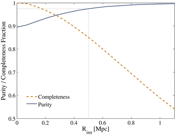
Figure 1. Purity and completeness of a mock sample of MW-like galaxies as a function of changing isolation radius, Riso. The mock galaxies are based on halos and subhalos in a high-resolution N-body simulation, with similar cuts applied as to the data sample. Over 95% purity is achieved for a cut of Riso = 0.5 Mpc.
Download figure:
Standard image High-resolution imageFor comparison with observations, we identify MW-sized halos (in the range of 1012 M☉ to 2 × 10¹² M☉) and compute the projected distance Rℓ to the nearest larger halo within a redshift range of ±1000 km s−1 (projected distances are calculated in the x–y plane, and redshift-space distances are calculated using halo positions and velocities along the z-axis). An MW-sized halo is classified as a satellite if it is within the virial radius of a larger halo; otherwise, it is classified as a host. Thus, for a given Riso, the completeness is calculated as the fraction of MW-sized host halos with Rℓ > Riso, and the purity is the fraction of hosts within the set of MW-sized halos with Rℓ > Riso.
As one would expect, as Riso increases, our sample becomes more isolated, and purity improves, but this is at the expense of rejecting truly isolated systems from our sample. Relatively high purity is important to us as it impacts the relevance of our results to the MW. However, a more complete sample will improve our resilience to selection effects. The choice for Riso thus seeks to maximize completeness while holding impurities to an acceptably low level. The results of our N-body investigation are encouraging. An isolation radius of 500 kpc (which would count the MW as isolated, since M31 is ∼700 kpc distant) gives purity above 95%, while still permitting a completeness of ∼85%. We therefore fix Riso at 0.5 Mpc for the core of our analysis and obtain a sample of 22,581 isolated MW analogs, extending out to z = 0.12 (in stripe 82, with fainter magnitude limit, we get 1946 MW analogs out to z = 0.15). We show in Section 5.3 that our results are stable upon variation of the isolation radius, which implies that impurities at the few-percent level do not have a significant effect. We also require that all potential MW analogs be at least a distance Riso away from the edge of the observed region. Since we are working at low redshift, the narrow southern SDSS stripes provide little useful area for our analysis, and so we neglect them.
2.3. Analogs of the Magellanic Clouds
The LMC and SMC are 2.4 and 3.8 mag fainter, respectively, than the MW in the V band (van den Bergh 2000). Since the V and r bands overlap strongly, similar magnitude differences will hold in r. To find analogs of the LMC and SMC, we thus search for galaxies around our isolated hosts within an aperture of physical size Rsat on the sky, and with apparent magnitudes in the range mhost + 2 to mhost + 4. (We work in apparent magnitudes to enable the use of the full SDSS photometric catalog, since the magnitude difference between satellites and their hosts should be the same in apparent or absolute values.)
The appropriate choice of Rsat is not entirely clear. The virial radius of simulated dark matter halos similar to MW is ∼250 kpc (Busha et al. 2011a), so that might seem a reasonable value. On the other hand, the LMC and SMC are both within 100 kpc of the MW (at distances of 50 and 63 kpc, respectively; van den Bergh 2000), so if we truly want MW analogs, we might prefer a lower value of Rsat ∼ 100 kpc. The closeness of the LMC and SMC is likely to be happenstance, however, and an overly restrictive value for Rsat could lead us to underestimate the abundance of MW–MC analogs.
A further consideration in choosing Rsat is contamination from background objects. Our primary analysis searches for satellites in the photometric catalog relies on statistical subtraction of background contamination. As is discussed in Section 3.4, before counting potential satellites, we use photometric redshift information to exclude a large fraction of the background objects. This cut is necessarily quite conservative, however, to avoid excluding true satellites from our sample, so significant background remains. The larger Rsat becomes, the higher the background contamination becomes, and the larger the statistical noise it induces in our results, as discussed in Section 4.1. We will thus want to keep Rsat as small as is reasonable, to maximize our precision. For our primary analysis, we set Rsat = 150 kpc, which strikes a reasonable balance between these different considerations. In Section 5.3, we explore the impact of varying Rsat and find it to be small but not insignificant.
Deblending is a final concern. If a satellite is very close to its host (either physically or in projection), the SDSS reduction pipeline might not identify it as a separate source. Thus, when we perform background subtraction to obtain a spherical search volume for satellites in Section 3.2.2 below, we are actually considering a bead-shaped volume, with a cylinder of radius of order 10 kpc (roughly the radius of an MW analog) removed from the center. Since Rsat is much larger than the size of a typical host galaxy, however, this cylinder represents ≲ 1% of the search volume (Figure 2 gives a visual impression of the relative distances involved). The impact of deblending on our results should therefore be negligibly small, and we neglect it in what follows.
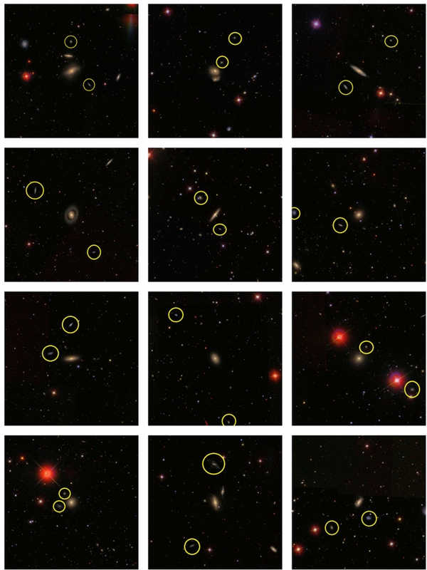
Figure 2. Images of selected MW-like hosts with exactly two MC-like satellites in the SDSS spectroscopic catalog, identified as those objects within a radius of 150 kpc and within 300 km s−1 of the host. Each image is scaled to 300 physical kpc on a side, centered on the host galaxy. Satellites identified as MC-like companions are circled in yellow. The 1st, 2nd, 4th, and 11th images (counting from left to right, top to bottom) show at least one bright, close companion to the MW-sized host. Image 11 shows two such objects at the same redshift as the central galaxy. In each of these cases, the companion is recognized as a satellite of the host but is too luminous to meet our criteria for being an MC-like satellite. The 5th, 6th, 8th, 9th, and 11th images feature prominent background objects with spectra at dissimilar redshifts. Background objects without spectra are clearly visible in every panel. The 5th and 12th panels exhibit fiber collisions. The blue object next to the upper left MC-like satellite in panel (5), though bright enough, did not have its spectrum collected or analyzed, similarly, the object to the right of the bluer MC-like satellite in panel (12) has no redshift or absolute magnitude information due to fiber collisions.
Download figure:
Standard image High-resolution image2.4. A Preliminary Analysis: Magellanic Clouds in the SDSS Spectroscopic Catalog
In this section, we generate preliminary results working exclusively within the SDSS spectroscopic catalog. This data set includes only the brightest objects (r < 17.77) in the survey, for which spectra were obtained. Although these results will be subsumed by a more precise and systematically robust result using photometrically selected satellites, we include the brief analysis to illustrate the conceptual simplicity of our main undertaking as well as to motivate the search in the deeper photometric catalog.
Though the stated magnitude limit of objects in the spectroscopic catalog is r = 17.77, we trim the set at r = 17.60 to avoid selection complications near the completeness limit that arise from recalibrations of the photometry since the main sample was selected. This limit applies to all satellites, which implies a minimum magnitude limit of r = 13.60 for hosts if we allow MC-like satellites to be 4 mag dimmer than their hosts.
The brightest 199 members of the MW-sized galaxies selected using the host-finding procedure outlined in Section 2.2 (with Riso = 0.5 Mpc, ΔMiso = 0) have redshifts between 0.01 and 0.026 and r-band magnitudes between 12.05 and 13.60 (SDSS units). The search conducted around these 199 MW-like hosts identifies as MC-like any galaxy with (1) absolute magnitude (Mv) between 2 and 4 mag dimmer than the magnitude of the host, that is (2) lying within a physical projected radius of 150 kpc of said host, and (3) has a redshift within Δzmax of the redshift of the host. The redshift difference Δzmax = 0.01 is equivalent to a ∼300 km s−1 velocity dispersion, chosen as a reasonable upper bound for the line-of-sight relative motion between an MW host and potential satellite.
The value of Δzmax also sets the uncertainty in line-of-sight position of any potential satellite, such that the geometry described by our limits is not a sphere centered on the candidate host but a cylinder with the same projected dimensions. The cylinder has a half-length of approximately 3 Mpc (as it happens, this is roughly the correlation length of an MW-luminosity host), and any interloper galaxies within it are indistinguishable from a true satellite. A systematic correction would be needed to convert this result to expected counts within the desired spherical region with radius Rsat (see Section 4.2.2). We do not perform the correction here because the precision of our results is already limited by our small sample size. SDSS fiber collisions will introduce a further source of systematic error for which we would need to correct, although this is likely to be small since the 55 arcsec SDSS fiber-collision radius corresponds to only ∼2% of the search cylinder for a typical spectroscopic host. A more careful analysis of the spectroscopic data in the case of LMC analogs is also in preparation by a different set of authors (E. Tollerud et al. 2011). In any case, we will derive more precise, systematically corrected results from the photometric sample in what follows.
Here, we simply quote the result for objects with MC-like properties found within the cylindrical redshift-space volume described above. This method, though failing to provide the desired search geometry, corresponds most closely to the results obtained in other spectroscopic searches for satellites (e.g., Zaritsky et al. 1993; James & Ivory 2011), with which our results are broadly consistent. It also has the advantage of exact identification of individual correlated objects (unlike our results in what follows, which are purely statistical). Figure 2 shows a mosaic of some likely MW–MC-like systems identified in the spectroscopic catalog using this procedure. In all, from these 199 hosts, we find that 132 (or 66.3%) have zero, 51 (or 25.6%) have one, 16 (or 8.0%) have two, and none have more than two MC-luminosity galaxies within the search cylinder. This number-count distribution is compared with the equivalent results from our larger photometric samples in Figure 9. Even without careful systematic correction, this result stands as qualitative confirmation of simulations (e.g., Boylan-Kolchin et al. 2010; Busha et al. 2011b) showing that MW-like halos have two MC-like satellites less than ∼10% of the time.
3. METHODS
In the last section, we motivated the need to move beyond the SDSS spectroscopic sample to obtain statistically robust results. The easiest way to obtain a larger sample is to make use of the deeper SDSS photometric catalog. Without precise redshift information, our analysis will depend on careful background subtraction, since line-of-sight projection effects conflate actual satellites with background objects. In essence, we trade the ability to identify individual satellites around a host for a substantial increase in statistical power. As discussed in Section 3.4, we can make the task somewhat easier by using photometric redshifts to exclude obvious background objects, but the photo-z's do not have sufficient precision to identify line-of-sight interlopers on a system-by-system basis. We introduce here an ensemble treatment of background subtraction performed on our expanded set of MW hosts.
Our desired result is the probability distribution function p(S), the probability that Nsat MC-like galaxies are present within Rsat of an MW-sized galaxy. We arrive at our measurement via a four-step process, as outlined below.
- 1.We count the total number of galaxies, T, around each candidate host that meet our magnitude and projected angular distance (Rsat) selection criteria (see Section 2.3). We use these to build a normalized probability distribution, the composite counts probability distribution function (PDF), p(T).
- 2.We estimate the PDF of the background "noise" counts, p(B), by counting galaxies meeting our satellite criteria in fields that do not contain an MW-analog host. The selection of these noise fields has important implications for the systematic uncertainty in our final result, so we take two quite different approaches to constructing them (see Section 3.2), estimate the systematic errors in each case, and check that the results are consistent.
- 3.We extract the desired signal PDF p(S) via deconvolution. Assuming signal and noise to be independent, the distribution p(T) measured in step 1 is simply the convolution of p(S) with p(B); thus, a straightforward deconvolution in Fourier space is all that is necessary to reconstruct p(S).
- 4.We estimate and correct for systematic effects that arise from catastrophic photo-z errors and from misestimation of the background contribution owing to large-scale structure, finally arriving at our best estimate for p(Nsat), the probability of an MW analog's hosting N MC-like satellites.
3.1. Composite Counts
In Section 2.2, we presented our process for selecting 22,581 MW analogs. Each host serves as the center of an individual search aperture, whose angular size varies with the host redshift but always corresponds to a transverse physical distance Rsat. For each aperture, a tally is made of all objects which fit our criteria for LMC/SMC-like satellites (e.g., having apparent r-band fluxes between 2 and 4 mag fainter than the host, in our baseline analysis). The normalized histogram of these total number counts is denoted by p(T); it represents our primary measurement in this study.
3.2. Background Estimation
To estimate the PDF of background number counts, p(B), we take a similar approach to earlier studies (e.g., Holmberg 1969; Lorrimer et al. 1994). In brief, we count galaxies that meet our satellite selection criteria, within comparison regions on the sky that do not contain a galaxy that meets our selection criteria for hosts (but that otherwise meet the isolation criteria). Previous authors taking this approach made use of data from photographic plates, and they wisely used comparison regions on the same plate as their host galaxies, so the comparison regions were quite nearby the hosts. In our case, we have access to a large, well-calibrated photometric survey field, so it is possible to choose comparison regions that are arbitrarily distant from the hosts. Since the estimation of background noise will be the dominant source of systematic error in this study, it is important to carefully consider the choice of comparison fields. We take two different approaches, which are subject to different sources of systematic error, in order to test the robustness of our results.
3.2.1. Isotropic Background
The simplest, most naive approach is to estimate the background from random locations on the sky. More specifically, we randomize the sky positions of our host sample within the SDSS NGC region. It is important for the sake of comparison that the search is performed on an identical distribution of aperture sizes and reference magnitudes, however, so we do not randomize the host redshifts or luminosities. Approximately 25,000 randomized sky positions are generated and each is associated with a set of object properties (absolute magnitude, apparent magnitude, redshift) belonging to a randomly chosen target host.
These search centroids are then subjected to identical isolation conditions as the targets with an additional constraint. As before, no search center may be within Riso of a brighter object than the host from which the search parameters were derived. Now, in addition, no search center may be within 2 Rsat of any MW-sized galaxy that is within 1000 km s−1 of the search redshift, as we hope not to contaminate our noise profile with signal. The histogram of counts of MC-like objects around these locations is then used to generate the isotropic background PDF, p(Biso).
This is likely to be an underestimate of the background around our hosts, however. Because galaxies are clustered, regions around hosts are generally denser than average, with a typical correlation length many times longer than Rsat of this study or even Rvir of a galaxy. Thus, though we have measured the random background noise, one would expect the total noise in our search apertures to be above random due to the contribution of projected correlated galaxies outside our region of interest described by Rsat.
If no correction is made for this effect, we have in essence counted all correlated objects within a cylinder of length roughly the correlation length r0 (see Figure 3), which is clearly an overestimate of the satellite population. Fortunately, it is straightforward to compute a correction for this systematic undersubtraction, via integrals over the galaxy correlation function. We derive this in Section 4.2.2 and will apply it to our results derived using the isotropic background estimate.

Figure 3. Schematic diagrams of our background subtraction procedures. (1) The two volumes corresponding to the center search aperture and the adjacent annulus are pictured. Red dots represent objects within actual physical distance Rsat of the host, green dots are objects outside Rsat but correlated with the host, and gray dots show random foreground and background objects. Simulations confirm that the amount of random and correlated background objects in the two volumes are approximately equal. (2) The result for random background subtraction is shown. The random background has been subtracted, but correlated line-of-sight structures remain, resulting in an effective cylindrical search volume (represented schematically by the green shaded region). (3) The result of annular background subtraction is shown. Both random and correlated line-of-sight objects have been subtracted. This is our best estimate of the desired result, the number of satellites within a radial distance Rsat of host.
Download figure:
Standard image High-resolution imageIt is worth noting, however, that a single correlation length (r0 ≈ 3 Mpc; Zehavi et al. 2010) along the line of sight corresponds to ∼300 km s−1 in redshift space; that is, it is the same length as the search cylinder we used for our preliminary spectroscopic analysis in Section 2.4. In other words, the results derived from isotropic background subtraction are roughly equivalent to our results in the spectroscopic catalog. Even in the case of perfect spectroscopic information, it is necessary to account for the presence of correlated objects along the line of sight if we wish to probe the true satellite population. Since we did not attempt to correct our spectroscopic result in Section 2.4, we will also present our uncorrected results for isotropic background subtraction, for the purpose of comparison.
3.2.2. Annular Background
It is also possible to estimate the random and correlated background simultaneously and directly by placing our comparison fields very close to the MW-analog hosts. In particular, we can estimate the background noise by counting galaxies that meet our satellite selection criteria in an annulus around each host galaxy, but outside the initial satellite search aperture, provided that the annulus has the same projected area as the center search region. (This technique is similar in spirit to the one that Chen et al. 2006 found to be optimal for interloper removal in spectroscopic data.) The histogram of counts in an annulus around each host then gives the correlated annulus background PDF, p(Bann).
A schematic diagram of this approach is shown in Figure 3, panel (1). The central column, with a sphere of radius Rsat cut out of it, has a slightly smaller volume than an annulus of the same projected area, so the counts in the annulus will tend to be slightly enhanced relative to the central cylinder. But, counteracting this, there is also, on average, a lower density of correlated objects in the annulus, owing to the larger distance from the host. The two effects will cancel for some particular choice of the annular radius, although it is difficult to justify a priori a particular choice of this radius.
We can make some use of N-body simulations to help guide our choice. In particular, we make use of a mock galaxy catalog generated from abundance-matching galaxy luminosities from the low-luminosity survey of Blanton et al. (2005a) to dark matter halos in the Bolshoi simulation. With this catalog, we can perform selection cuts on MW hosts (luminosity and isolation criteria) identical to the ones we perform on observed SDSS galaxies. Then, we may compare the number of objects with luminosities similar to the LMC and SMC (i.e., 2–4 mag fainter than their host galaxy) in both cylinders with the inner spheres removed, and in hollow cylinders, as shown in panel (1) of Figure 3.
The most natural choice for the background-estimation annulus is the region immediately outside the search aperture, with R2sat < rann2 < 2 R2sat, which we will call Annulus I. In this case, tests from our mock catalogs show that the counts in the inner and outer cylinder are roughly equal, with the counts in the annulus possibly exceeding the counts in the search aperture, but by no more than ∼10%. If we move the annulus outward to 1.5 R2sat < rann2 < 2.5 R2sat (which we will call Annulus II), the annulus counts in the simulation appear to underestimate the aperture counts slightly, but again by no more than ∼10%.
Because the N-body models give only a rough approximation of our measurements in SDSS, and because we would prefer not to rely too heavily on simulations for our observational results, we do not attempt to further optimize the radius of our search annuli. Instead, since our two annuli appear to tightly bracket the optimal one, we will take the results using Annulus I to be our primary results, and we will compare to the results using Annulus II to estimate the size of the residual systematic uncertainty.
3.3. Signal Extraction Via Deconvolution
We make the assumption that the number of actual satellites to be found around an MW-sized galaxy is unrelated to the number of background objects which might be projected into the same aperture. That is S, the signal, and B, the noise, are independent variables. Their sum is a third random variable, T = S + B. This implies that the probability distribution of T is just the convolution of the S and B PDFs:
where the * symbol indicates convolution.
By using the methods described in Sections 3.1, 3.2.1, and 3.2.2, we have precise measurements of p(T), p(Biso), and p(Bann), respectively. We are interested in p(Scor), the probability of encountering Scor LMC/SMC-like correlated galaxies within a cylinder of radius Rsat centered on an MW-sized host. This is computed by deconvolving p(Biso) and p(T). More importantly, we wish to obtain p(Ssat), the probability of encountering Ssat MC-like satellites within a sphere of physical radius Rsat around such a host. This can be derived by applying a systematic correction to p(Scor) (see Section 4.2.2) or by deconvolving p(Bann) from p(T).
The deconvolutions take place in three steps. First we transform into Fourier space using a fast Fourier transform (FFT; this is indicated by the operator  below). Then a convolution is simple multiplication:

By rearranging this equation we obtain  , and an inverse FFT retrieves p(S) in each case. For an example (and a preview of our results), see the left-hand panel of Figure 7. There, the blue curve (p(T)) can be obtained by the forward convolution of the red curve (p(B)) with the green curve (p(S)) as in Equation (1). In practice, we have measured the red and blue curves and deconvolved them via Equation (2) to extract the green curve.
3.4. Use of Photometric Redshifts
As discussed below, the statistical errors in p(S) depend strongly on the typical number of background (noise) galaxies in the search aperture. We can therefore greatly improve the precision of our results by making use of photometric redshift information to exclude obvious background galaxies before we begin the satellite-counting exercise outlined above. Because photometric redshift estimates are highly prone to catastrophically large errors—especially for faint galaxies—we do not attempt to use photo-z's to identify the actual satellites of individual hosts; instead, we merely use them to make a conservative initial background cut.
Best-fit photometric redshift values and p(z) probability distributions are computed by Cunha et al. (2009) for each photometric object and are made publicly available on the SDSS DR7 Web site. We make a cut in the imaging catalog on best-fit photo-z at some threshold value zphot, max and exclude galaxies with higher photo-z's from our sample. Because photo-z estimates are prone to inaccuracies and particularly to catastrophic errors, any cut on zphot will wrongly exclude some number of galaxies that are actually satellites at low redshift. This will introduce a systematic undercounting of satellites around MW-analog hosts.
We would like our sample of low-redshift galaxies to be as free as possible of background objects, to reduce our statistical errors, while also being highly complete, to minimize systematic errors. However, increasing zphot, max increases the background noise and worsens our statistical errors, while reducing zphot, max rejects an increasing number of true satellites and increases our systematics. This trade-off is shown in Figure 4, where we have plotted the summed p(z) distributions for a representative set of possible MC-like galaxies with zphot above and below 0.23. There is a tail of high-photo-z galaxies that are actually located at z < 0.12 (dotted curve) and hence ought to be considered as potential satellites; their exclusion causes a systematic undercounting of satellites. There is also a large number of galaxies with zphot < 0.23 that have true z > 0.12 (solid line); these act as background noise and contribute to the statistical errors. In the next section, we derive in detail the impact of these two sources of error and their dependence on the photo-z threshold. We find that a value of zphot, max = 0.23 strikes a reasonable balance between the purity and completeness of satellites as the resulting statistical and systematic errors have roughly equal amplitude.
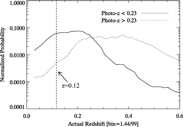
Figure 4. Distribution of true redshifts for two galaxy samples divided by photometric redshift. The dashed histogram indicates the average normalized p(z) distribution from Cunha et al. (2009) for galaxies with zphot > 0.23, and the solid histogram is the same distribution for galaxies with zphot < 0.23. By comparing the amplitude of the two curves at z < 0.12, it is possible to estimate the relative numbers of potential z < 0.12 satellites that are kept (solid line) and excluded (dashed line) by our photo-z cut. These differ by roughly an order of magnitude, so the required systematic corrections to our satellite counts are expected to be on the order of 10%.
Download figure:
Standard image High-resolution image4. ERROR BUDGET
4.1. Statistical Errors
The statistical uncertainty in our measured p(S) has three sources. The first is the overall size of our sample of MW-like host galaxies: as our sample size increases, we expect that the precision of our result should improve as well, owing to reduced Poisson noise. More specifically, the uncertainty in our measured composite counts PDF, p(T) should be purely Poisson at each value of T. The second source of error is noise from the background: if we increase our photometric redshift cut, we increase the number of background galaxies in our total composite counts and hence we reduce the signal-to-noise ratio of our final measurement. More specifically, the isotropic background PDF, p(B) is a source of noise that propagates through our analysis in Fourier space to our final measurements for p(S). Our sample size is large enough in our primary analysis that we are dominated by this second source of error.
A final source of statistical error may arise from sample variance (also sometimes called cosmic variance). Although our observational regions are likely numerous enough that this is not a dominant source of error, it is possible that the variance in our composite or noise counts exceeds simple Poisson noise. To fully characterize the variance in our sample, therefore, we use the jackknife technique to estimate the errors on our measured p(T) and p(B). We divide our spatially contiguous set of MW-sized hosts into 50 subsets, each of which may contain a different number of galaxies but occupy an equal area on the sky. In each iteration, a different subset is omitted, and 49 of the 50 tiles produce a normalized PDF of counts (composite or noise). The result is 50 different values for each histogram bin. Their mean is the unbiased PDF; error on the mean is approximately  , where σi is the standard deviation in each bin, i.
It is possible in principle to propagate these uncertainties analytically through the Fourier analysis to obtain final errors on p(S). However, the scalings involved are rather non-intuitive, and the calculation is prone to numerical instabilities when the p(B) and p(T) distributions are truncated at some maximum abscissa value, which is typically necessary. Therefore, we propagate uncertainties through the deconvolution using a stochastic approach. The same FFT deconvolution is performed approximately one million times, each time with a set of values for p(T) and p(B) randomly drawn from Gaussian distributions with the means and standard deviations found in the jackknife analysis. To mute the effects of ringing in the deconvolved result, we keep only those trials whose resulting probability densities are nonnegative everywhere. The median in each bin of the satellite counts PDF is our result for an MW-sized galaxy's probability of hosting S = 0,1,2,3... MC-like satellites. Error bars bracket the 68% confidence interval.
Following this procedure, we find that the stochastic error bars derived on p(S) are much larger than the error bars estimated for p(T) or p(B) in our jackknife analysis. This indicates that the error in p(S) is dominated by background noise, rather than counting statistics. When we are in this regime, increasing our sample size by a factor of order unity will not shrink our error bars as  . Instead, our errors will thus scale roughly as the average signal-to-background-noise ratio, 〈S〉/〈B〉. To improve our errors, we would need to reduce the background, for example by making a stricter photo-z cut (however, doing this would increase our systematic errors, as discussed in the next section). Because we are not limited by our sample size, we have taken an aggressive approach in our selection to excluding objects near the edges of the NGC region.
To illustrate the scaling of our uncertainties, we compute our errors for different values of 〈S〉/〈B〉. We can directly obtain 〈T〉 and 〈B〉 from our basic number-count measurements. Regardless of the shape of the PDFs, this equation should then hold

The most direct way of varying the signal-to-noise ratio is by shifting the maximum photo-z cut mentioned in Section 3.4. Since the bulk of objects with zphot > 0.12 are background objects, changing zphot, max changes 〈B〉 while holding 〈S〉 roughly steady. Between 0.17 < zphot, max < 0.29, our signal-to-noise ratio varies from approximately 0.27 to 0.15. For our adopted value, zphot, max = 0.23, 〈S〉/〈B〉 = 0.18.
Figure 5 plots the size of the error bars on p(S) (computed as described in Section 4.1) against the choice of photo-z cutoff and resulting 〈S〉/〈B〉 for S = 0, 1, 2. The relationship between the photo-z cutoff and the statistical uncertainty in our results demonstrates the need for a maximum photo-z limit on the Sloan imaging catalog in our analysis. 〈S〉/〈B〉 also varies with the search aperture size Rsat, though this relationship is more complicated, since the average signal (number of satellites) depends on Rsat as well.
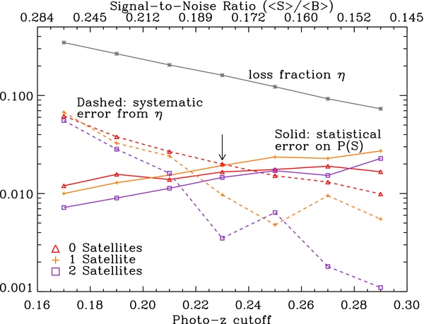
Figure 5. Various sources of uncertainty in our analysis and their scaling with photo-z cutoff. The absolute statistical uncertainty on P(S) increases as the photometric redshift cutoff increases and the average signal-to-noise ratio decreases. This is shown by the colored solid lines, for S = 0, 1, 2. Here "signal" is the average number of MC-like satellites per Galaxy-sized host and "noise" is the background contaminating objects. A competing systematic effect arises from true satellites with inaccurate photo-z's, which are improperly rejected by our photo-z cut. The fraction of true satellites excluded in this manner is shown by the gray line, and the resulting systematic error is given by the colored dashed lines. Our adopted photo-z cutoff, indicated by the arrow, is chosen to approximately balance these two sources of error.
Download figure:
Standard image High-resolution image4.2. Systematic Errors
There are two primary sources of systematic error in our analysis. First, some fraction of true satellites will be subject to catastrophic photo-z errors and thus will be wrongly rejected in our background-exclusion cut. This will always cause a slight undercounting of satellites. Second, our isotropic background estimation in Section 3.2.1 assumes that background galaxies are completely uncorrelated with the MW-analog hosts. Since galaxies are in fact well known to be correlated, this technique will lead to a slight overcounting of satellites from correlated objects along the line of sight. We address these two sources of systematic error in turn below.
4.2.1. Photo-z Losses
To estimate the error caused by the photo-z cut in Section 3.4, we use the p(z) information from Cunha et al. (2009) to compute a loss fraction, η. This is the average probability that any potential satellite object (that is, an object with the appropriate properties and actual redshift z < 0.12) will be cut out of our sample owing to a catastrophic photo-z error.
Photo-z's of dimmer galaxies are more error-prone than those of brighter objects since the photometric errors are larger. Thus, an average loss fraction must be computed on a sub-sample of galaxies representative of the apparent magnitude distribution of our potential satellites. We construct this sample by iterating over our MW-analog hosts and, for each host, randomly selecting 1000 galaxies that are 2–4 mag fainter and adding them to our sample (this means that individual faint galaxies will appear more than once in our sample, but this allows us to obtain the correct magnitude distribution). We operate on this set by dividing it into two, those objects with best-fit photo-z above the threshold zphot, max, those objects with best-fit photo-z below this cut (see Figure 4).
Then, if L is the set of all potential satellites with best-fit photo-z below zphot, max, the loss fraction is

Since we do not have direct access to the actual redshifts, zg, of individual photometric objects, we use Bayes's Theorem to rewrite the conditional probability in a more accessible form:
In Figure 4, L is represented by the solid line, and the set of all other objects, which we can call M, is represented by the dotted line, so  is the integral under the dotted line between z = 0 and z = 0.12.
  is the ratio between the size of M and the size of the full set M∪L, and p(zg < 0.12) is the integral from z = 0 to z = 0.12 of the normalized p(z) distribution of M∪L.
The galaxy completeness after the photo-z cut, 1 − η, is plotted against zphot, max in Figure 6. For our primary results searching in the main Sloan imaging catalog with zphot, max = 0.23, η = 0.16. We thus expect the impact of this first source of systematic error to be at the ∼10% level.

Figure 6. Completeness of z < 0.12 objects (i.e., the fraction of z < 0.12 objects with zphot < zphot, max) as the maximum photo-z cutoff, zphot, max, is increased.
Download figure:
Standard image High-resolution imageGiven an estimate for η, we can compute a straightforward correction for the systematic error from photo-z losses. We relate pmeas(S), the measured probability distribution for MC-like satellites around MW-like hosts, to ptrue(N), the actual distribution, applying the overall loss-fraction, η, uniformly as a loss probability for each satellite and including appropriate combinatorial factors. For a galaxy with N actual satellites, the probability that exactly m satellites will be lost is
Then the measured satellite PDF is related to the true PDF by

This equation corresponds to a formally infinite system of equations, one for each value of N. Since pmeas(S) and (presumably) ptrue(N) approach zero as N increases, however, we may solve for ptrue(N) by truncating at some appropriately large values of N and S (chosen to be 15, well beyond where the average value is zero). This gives a tractable system of equations, which we then solve to obtain a result corrected for photo-z losses.
4.2.2. Large-scale Structure Effects
To estimate the impact of correlated structure along the line of sight, we would like to compute an analogous quantity to the loss fraction, η—we will call it the boost fraction, ζ—that quantifies the fraction of our satellite counts that can be attributed to line-of-sight structure after we have made an isotropic background correction. To do this, we make use of the galaxy autocorrelation function ξ(r), which quantifies the excess probability above random of finding a galaxy some distance r from another and which is well measured in the local universe. Strictly speaking, since we are considering the correlations between two different galaxy populations, we should use the cross-correlation function of these two samples, but given that both MW-sized objects and LMC-sized objects should be roughly unbiased tracers of the dark matter distribution (e.g., Zehavi et al. 2010), their cross-correlation and autocorrelation functions will be approximately equal.
In particular, we can make use of the projected correlation function wp(rp), which is given by integrating ξ(r) along the line of sight. This function gives the excess probability (above random) of finding a galaxy at a projected distance rp away from another on the sky. At rp < Rsat, the dominant contribution to wp(rp) is from true satellite galaxies, but there will also be some contribution from unbound galaxies along the line of sight. We can estimate the size of this contribution by integrating ξ(r) along the line of sight, excluding a sphere of radius Rsat around the origin and comparing this to the full wp(rp). Following Davis & Peebles (1983), the modified projection we want is
where the lower limit of integration is
and defines the sphere within which we wish to count satellites. This can be integrated numerically for a given choice of ξ(r).
If we let Rsat → 0 and assume a power-law form for the correlation function, ξ(r) = (r/r0)−γ, we obtain the well-known analytic formula for wp(rp),
Then, by integrating both  and wp out to Rsat, we can compute the probability that a satellite candidate is correlated with its putative host, beyond what is accounted for by our isotropic background correction, but is not actually within Rsat. This probability is the boost fraction ζ:
Assuming γ = 1.8 (approximately the value for galaxies dimmer than L*; e.g., Zehavi et al. 2010), when Rsat = 150 kpc we obtain ζ = 0.21.
The probability that exactly n correlated galaxies will be counted along the line of sight is then

The second factor ensures that the probability distribution is normalized (since the sum over n is a geometric sequence); it accounts for the probability of having zero correlated line-of-sight systems. The systematic correction for correlated structure can then be derived, as in the previous section, by relating the measured PDF to the true PDF:
We can solve this as before by truncating the formally infinite system of equations at suitably large S such that pmeas(S) vanishes. In practice, we first compute the correction for photo-z losses from Equation (7) and then we compute the boost correction using the results of that calculation. This ensures that we account correctly for correlated non-satellite galaxies that were lost to photo-z failures.
Before moving on, we make note of a possible inaccuracy in the analysis in this section. We have assumed that ζ does not depend on the true number of satellites, N. However, since ζ depends on the bias of the hosts, this may not be completely correct. One might imagine that the satellite population depends, to some extent, on the formation epoch of the hosts (since hosts forming earlier have more time to disrupt or merge with their satellites). Galaxy biasing is also known to depend on formation epoch (the so-called assembly bias), and this effect is at the ∼20% level for halos like the MW (Wechsler et al. 2006). In fact, Busha et al. (2011b) show explicitly that there is some dependence of the satellite number on environment in this mass regime. ζ will depend linearly on the host bias via the host-satellite cross correlation function. However, including this effect would complicate our analysis substantially: we would no longer be able to separate Equations (7) and (13), and we would have to write them as a double sum, yielding a much more complicated system of equations. Because the effect is of order 20% on top of a boost fraction that is of similar order, we treat it as a second-order correction and neglect it.
5. RESULTS
5.1. Primary Results
To compute our main results, we use the parameters Riso = 0.5 Mpc, ΔMiso = 0 (i.e., only rejecting galaxies as non-isolated if they have a brighter companion), ΔMsat = 2 (searching satellites 2–4 mag dimmer than host), Rsat = 150 kpc, and zphot, max = 0.23. The maximum photo-z value is chosen to yield random errors that are greater than or similar to the systematic errors from photo-z losses (see Figure 5), as discussed in Section 4.2. We note that our isolation and satellite-search parameters would select the MW–LMC–SMC system, since our nearest bright neighbor, M31, is 0.7 Mpc distant, and the LMC and SMC are both well within 150 kpc of the MW. In what follows, we will vary these parameters to check the robustness of our results; we find the satellite counts to be relatively insensitive to the choice of parameters.
In Figure 7 and Tables 1 and 2, we report the percentage of MW-sized galaxies with N satellites or correlated objects centered on the host. N takes on integer values, and is labeled Ncor for the result accomplished through isotropic background subtraction and Nsat for the result achieved through annular background subtraction.

Figure 7. Probability that an MW-sized galaxy hosts Nsat LMC/SMC-like satellites or Ncor line-of-sight correlated structures. Left: our primary result, p(Nsat) (solid green points) computed using annular background estimation, along with the various steps involved in deriving this result, described in Section 3. The blue curve shows the composite counts PDF, p(T) and the red curve shows the background counts PDF estimated from annuli around each MW analog. The green curve is the deconvolution of these two PDFs, p(S), and the green data points are the values for p(Nsat) after correction for photo-z losses. Right: similar curves are shown, but now for the case of isotropic background estimation. Now the orange curve is the deconvolved p(S) and the open orange points are p(Ncor) after correction for photo-z losses. Solid orange points show our best estimate for p(Nsat) in this case, after computing a correction for correlated structure along the line of sight. We find that these results compare favorably to the results from left panel (green points and curve), which suggests that our results are robust. The host and satellite selection parameters used in this analysis are Riso = 0.5 Mpc, Rsat = 150kpc, zphot, max = 0.23 (η = 0.16), and ΔMiso = 0.
Download figure:
Standard image High-resolution imageTable 1. Percentage of MW-luminosity Host Galaxies with N LMC/SMC Luminosity Satellites within a Sphere of Radius 150 kpc, for N = 0–6
| Satellite | Measured % | Systematic Loss | Annulus Systematic |
|---|---|---|---|
| Counts | of MW Analogs | Adjustment | Uncertaintya |
| Zero | 83.4+1.5 − 1.4 | −2.0 | −4.2 |
| One | 10.8+1.8 − 1.6 | +0.8 | +2.6 |
| Two | 3.1+1.3 − 1.5 | +0.4 | +1.6 |
| Three | 1.4+0.9 − 1.0 | +0.2 | +0.1 |
| Four | 0.7+0.6 − 0.5 | +0.4 | +0.2 |
| Five | 0.1+0.2 − 0.1 | +0.2 | +0.1 |
| Six | 0.1+0.2 − 0.1 | −0.1 | +0.1 |
Note.a This is our estimate for the maximum additional correction that might be required to account for having chosen a non-optimal annulus for background estimation.
Download table as: ASCIITypeset image
Table 2. Percentage of MW-luminosity Host Galaxies with N LMC/SMC Luminosity Correlated Objects within a Cylinder of Radius 150 kpc, for N = 0–6
| Correlated | Measured % | Systematic Loss | Systematic Boost |
|---|---|---|---|
| Objects | of MW Analogs | Adjustment | Adjustment |
| Zero | 69.7+1.6 − 1.3 | −3.8 | +16.5 |
| One | 21.1+1.7 − 1.9 | +1.0 | −11.1 |
| Two | 6.8+1.5 − 1.5 | +2.1 | −3.4 |
| Three | 1.3+1.0 − 0.7 | +0.2 | −1.8 |
| Four | 0.6+0.7 − 0.5 | +0.3 | −0.1 |
| Five | 0.1+0.3 − 0.1 | +0.1 | −0.1 |
| Six | 0.1+0.2 − 0.1 | −0.0 | −0.1 |
Download table as: ASCIITypeset image
Our annular background-subtraction technique gives our best estimate for the counts of dwarf satellites within a sphere of radius Rsat centered on each MW-sized host. We find the probability of there occurring Nsat = 0, 1, and 2 bound MC-like satellites to be (81.4 ± 1.5)%, (11.6 ± 1.8)%, and (3.5 ± 1.4)%, respectively, after adjustment for systematic errors arising from catastrophic photo-z failures (see Section 4.2.1). The measured values and systematic corrections are tabulated in Table 1 and plotted in the left-hand panel of Figure 7 (green curve and data points). Also plotted in that figure are the composite counts PDF p(T) and the background PDF p(B) (blue and red curves, respectively) which are the curves that have been deconvolved to yield the measured satellite counts.
We derived these results using the comparison region immediately outside our search aperture that we called Annulus I in Section 3.2.2. As we discussed in that section, this may yield a very slight overestimation of the background, according to our tests in simulations. To quantify the potential size of this residual systematic error, we also compute our results using Annulus II (which simulations suggest is likely to yield a very slight underestimate of the background). We take the difference between these two results to be an estimate for the maximum remaining systematic error in our primary results; we report this in the final column of Table 1.
The isotropic background correction yields counts of MC-like dwarf galaxies correlated with the host within a cylinder around the host with radius Rsat and effective half-length of roughly the correlation length of unbiased mass tracers. For Ncor = 0, 1, and 2, we find probabilities (64.6 ± 1.5)%, (22.8 ± 1.8)%, and (9.7 ± 1.5)%, respectively. These numbers have also had the systematic correction for photo-z loss applied; the measured numbers and the corrections are tabulated in Table 2 and plotted in the right-hand panel of Figure 7 (thick orange curve and open data points), along with the composite and background PDFs. As discussed in Section 3.2.1, this result is the most directly comparable to satellite counts measured in redshift space, if interlopers have not been accounted for, so we present it here for comparison to our results in Section 2.4.
In Section 4.2.2, we developed a further systematic correction to allow us to remove the effects of correlated line-of-sight structures from this result. We compute this correction for the results of the isotropic background subtraction, and we give the results in the final column of Table 2. We also plot the corrected probabilities in the right panel of Figure 7 (solid orange points) and compare to the results of our annular background correction (green points). The good agreement between these two approaches gives us confidence that our methods are robust. We note that a similar systematic boost correction could also be usefully applied to any future spectroscopic satellite searches to account for correlated interlopers.
Our results compare favorably with data from recent high-resolution numerical N-body simulations, such as the Millennium-2 simulation (Boylan-Kolchin et al. 2010) and the Bolshoi simulation. The latter agreement will be discussed in more detail in a companion paper to this one (Busha et al. 2011b). It is also worth mentioning that none of our measurements of p(Nsat) is consistent with a Poisson distribution with an expectation value of 〈N〉 = 0.3. A detailed discussion of this can be found in the companion paper (Busha et al. 2011b).
5.2. Satellite Populations as a Function of Host-galaxy Color
These results suggest that the MW, with two large, close satellites, is not a typical galaxy for its luminosity. Since the MW is a blue, star-forming galaxy, we can take the analysis one step further and investigate whether the number of satellites is a function of galaxy color. This may be quite worthwhile, since the SDSS sample is dominated by red galaxies, and this could complicate the implications of our study for the MW. Galaxy colors in the local universe are well known to be bimodal (Strateva et al. 2001), and we can cleanly divide our sample into red and blue objects by cutting at u − r = 2.4.
We repeat our analysis for the red and blue samples separately, using annular background estimation, and we find no statistically significant difference between the satellite statistics of the two sets. The results are provided in Table 3, where systematic adjustments for photo-z losses have been applied to the numbers given (the adjustments were not applied in Tables 1 and 2). This result appears to be at odds with work by Lorrimer et al. (1994) and Chen (2008), who found more satellites around early-type galaxies, on average, than around late-types. However, those studies considered a wider range in host luminosity than we have done here, and so it is likely that the early-type samples were skewed toward brighter magnitudes than the late-type sample. The fact that we find no significant difference in our larger sample, which is limited to a narrow range in host luminosity, suggests that the earlier results may have mainly uncovered a trend with host-galaxy luminosity, rather than galaxy type.
Table 3. Satellite Statistics of Red- and Blue-sequence MW-sized Galaxies, Using Annular Background Estimation and after Systematic Adjustment
| Number of | Red Galaxies | Blue Galaxies | Average |
|---|---|---|---|
| Satellites | P(Nsat) | P(Nsat) | P(Nsat) |
| Zero | 82.0 | 81.2 | 81.5 |
| One | 11.6 | 12.5 | 11.7 |
| Two | 2.6 | 3.5 | 3.5 |
| Three | 2.1 | 0.5 | 1.5 |
| Four | 0.8 | 1.3 | 1.1 |
| Five | 0.3 | 0.3 | 0.3 |
| Six | 0.0 | 0.0 | 0.0 |
Download table as: ASCIITypeset image
It is reasonable to wonder how our results change if we divide the satellite population by color, especially since the MCs are both blue, star-forming galaxies. However, since we do not have very accurate photo-z estimates for faint SDSS galaxies, we also lack good k-corrections for these objects, and so their absolute colors are uncertain. In order to produce robust and reliable results on the color dependence of the satellite population, more accurate photo-z estimates would be required. We therefore do not attempt to perform this test here.
5.3. Robustness of the Results
5.3.1. Varying the Selection and Search Criteria
In this section, we confirm the stability of our main results for the probability of finding Nsat MC-like satellites in a sphere of radius Rsat around an MW-sized host. We vary several key parameters defined earlier in Sections 2.2 and 2.3: Rsat (the satellite search radius), ΔMsat (the maximum satellite magnitude relative to the host), Riso (the host isolation radius), and ΔMiso (the host isolation relative magnitude limit). The first two parameters alter our definition of an MC-like satellite, while the latter two change what is considered a suitable MW-like host. We vary each of these parameters over a reasonable range of selection criteria that might be expected to produce an approximate analog of the MW–LMC–SMC system. The results of this investigation are shown in Figure 8, where each parameter is varied in turn, while holding the other parameters fixed at their nominal values.
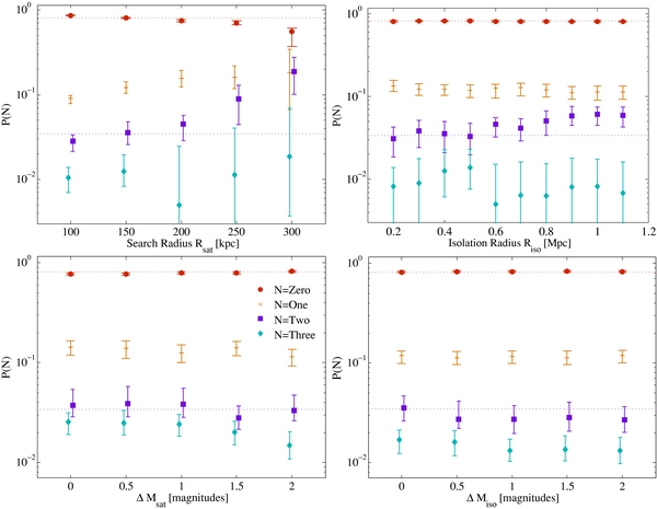
Figure 8. Sensitivity of the probability of hosting N = 0, 1, 2, or 3 satellites to changes in various selection parameters. In each panel, one selection parameter is varied and the others are held fixed at our nominal values that were used in Figure 7. Our results for the nominal parameter values are shown as dotted lines. Top left: dependence of probabilities on satellite search radius around the host galaxy. Top right: dependence of probabilities on variation of the isolation radius around the host galaxy, Riso. Bottom left: the allowed magnitude disparity between host and MC-like satellite, ΔMsat, is varied. Here, we search for satellites with magnitudes 2–4, 1.5–4, 1–4, 0.5–4, and 0.1–4 mag dimmer than host, plot is indexed by the changing minimum value. Bottom right: results with increasingly stringent host-neighbor relative brightness limit ΔMiso.
Download figure:
Standard image High-resolution imageAs would naively be expected, more satellites are detected as we increase the satellite search radius Rsat. However, the satellite counts are remarkably flat out to Rsat = 200 kpc. If we very stringently require candidate MCs to lie within Rsat = 100 kpc of their hosts (as the LMC and SMC do) then slightly less than 3% of MW-sized galaxies host two MC-like satellites. On the other hand, if we expand the search radius to 200 kpc, this fraction becomes about 5%. Even expanding it to 250 kpc (roughly the virial radius of the MW derived in Busha et al. 2011a), the fraction of hosts with two satellites rises only to ∼8%. This suggests that our analysis has largely captured the probability of true MC-analog satellites.
To further test whether we have captured the full satellite population in our main analysis, we compute the mean Nsat values in each of the radial bins shown in the upper left-hand panel of the figure. Taking the difference between these values, and assuming a spherical search geometry, we can then compute the number density of satellites in bins of radius. Because this measurement is nonnegative by construction, we expect that stochastic noise will cause us to measure a positive value in each bin; however, once we have measured the satellite population as completely as is possible within the uncertainties, the measured number density at all higher radii will be consistent with zero. In performing this exercise, we find that the measured average number density rises sharply below Rsat = 150 kpc and that it is roughly flat and consistent with zero at all higher values of Rsat. This confirms that our fiducial value of Rsat captures the MC-analog population as well as is possible within the uncertainties in our analysis.
In addition, a slight upward trend in the N = 2 value appears at the 1σ level as hosts become increasingly isolated from larger neighbors (upper right panel). If this weak trend is real, it is most easily explained as an effect of host formation history. More isolated hosts will have formed more recently, on average, so they will have had less time to disrupt or accrete their satellites, and so their satellite population will be enhanced relative to hosts in denser regions.
Lastly, we note that there is very little trend with the satellite relative-luminosity criterion ΔMsat (lower left panel of the figure), despite the fact that we are increasing the magnitude range considered by up to a factor of two. Since the overall galaxy luminosity function is not particularly steep over this magnitude range, one might expect the satellite probability to rise substantially when we broaden this search criterion. However, there is no particular reason that the luminosity function of satellites of MW analogs should the same as the overall luminosity function in this range. Our results suggest in fact that it is not. We may conclude from this result that satellites brighter than the MCs are extremely rare.
No other significant trends are observed under variation of host parameters. Specifically, little to no change in the results is evident if we reject hosts with companions slightly fainter than themselves. This is not particularly surprising, since such galaxies constitute only around one quarter of the sample in our primary analysis. Thus, we find our results to be quite robust to all significant and reasonable parameter changes; they are not simply an accident of the satellite search criteria we have chosen.
5.3.2. The Stripe 82 Co-added Catalog
We partially repeat the analysis for the deeper co-added data in the SDSS equatorial stripe (Stripe 82). The Stripe 82 catalog is not only deeper than the main SDSS imaging database (magnitude limit r ≈ 23.5) but has no spatial intersection with the Northern Galactic Cap, offering a disjoint set of objects with which we can verify the results. Because of the deeper photometric limit, we can consider potential MW-like hosts a bit dimmer, near to the completeness limit of the main SDSS spectroscopic sample, r = 17.60 (whereas we were limited to r = 17, 4 mag brighter than our photometric limit, in the NGC). Even with this deeper magnitude cut, there are only 1946 MW-sized galaxies in Stripe 82 that have spectra and meet our primary isolation criteria, compared to 22,581 in the NGC. This sample extends to slightly higher redshift: z = 0.15, rather than 0.12.
Since the statistical power of this sample is limited by its small size, we choose to compute only one of the results for comparison to the NGC sample. The simplest result to compute is the PDF of correlated galaxy counts, p(Ncor), calculated using isotropic background estimation. We have already shown that this result can be systematically corrected to accurately recover p(Nsat), and there would be no changes to this correction procedure in the Stripe 82 data set, so comparing this one result should be sufficient. The isotropic-background result also has the advantage of being most directly comparable to the spectroscopic analysis we performed in Section 2.4 (as explained in Section 3.2.1).
All the methods described earlier apply to this analysis except for the specifics of our choice of zphot, max and computation of the loss fraction η. A careful photo-z cut is even more important here, as the sky density of photometric objects in Stripe 82 far exceeds that of the main SDSS imaging catalog in the north. Here, we use photometric redshifts computed for the full Stripe 82 co-added catalog (R. Reis et al. 2011, in preparation) using the neural-network approach of Oyaizu et al. (2008). Lacking full p(z) estimates for this sample, we compute η from a subset of the photo-z validation set matched to the apparent magnitude and redshift distributions of our MC-like satellites. Objects in the validation set have measured spectroscopic redshifts but were not used to train the photo-z algorithm; they are used to test the accuracy of the photo-z estimates. We can make histograms of this data set to obtain p(z) distributions for different subsets and then perform an analysis analogous to Section 4.2 to obtain the fractional photo-z loss, η. We find that, for the Stripe 82 photo-z values, a cut of zphot, max = 0.21 corresponds to η = 0.15, which is acceptably small, so we use this maximum photo-z cut in our analysis.
The p(Ncor) results obtained from Stripe 82 are in good agreement with those obtained using the photometric catalog in the NGC in Section 5.1 and with the results computed using only spectroscopic information in Section 2.4. A comparison of the three p(Ncor) measurements is shown in Figure 9. Since disjoint data sets yield statistically identical results despite covering disparate ranges in redshift and apparent magnitude, and despite having photo-z-induced systematic errors computed with different algorithms, we can be confident that our results do not depend strongly on these details.
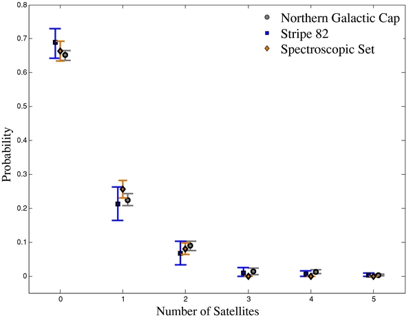
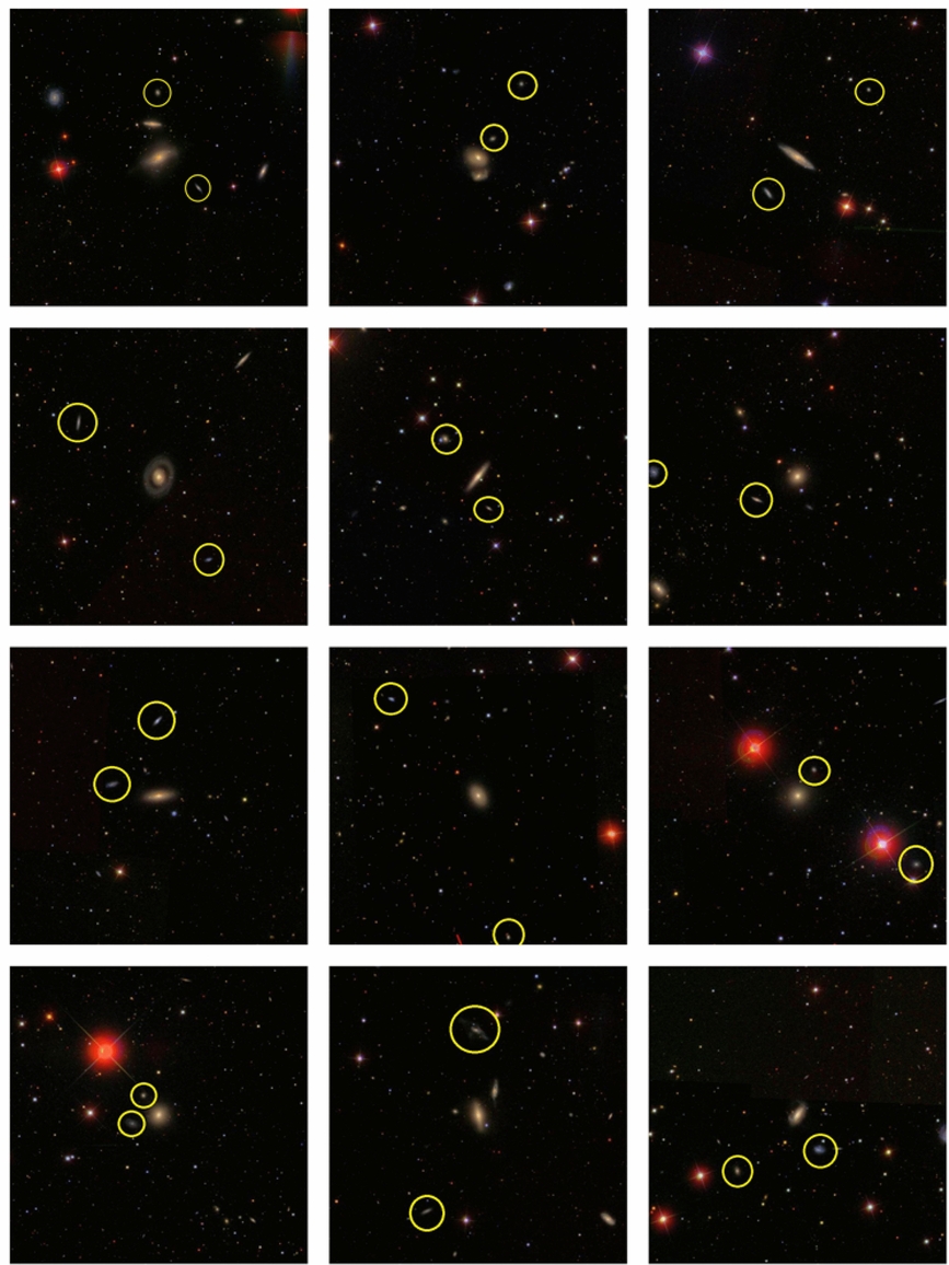
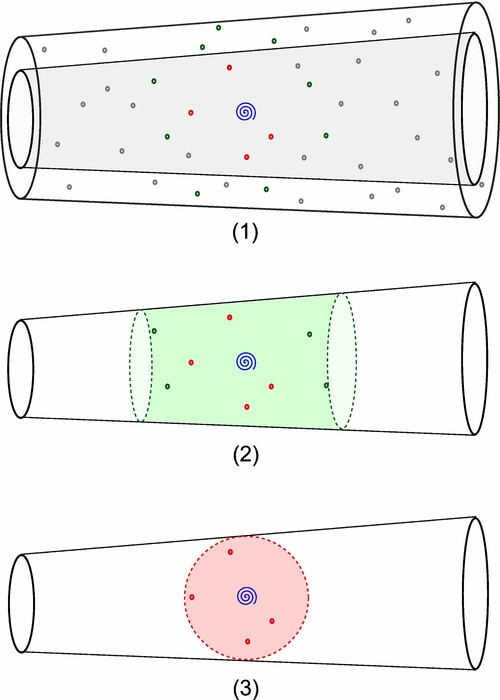
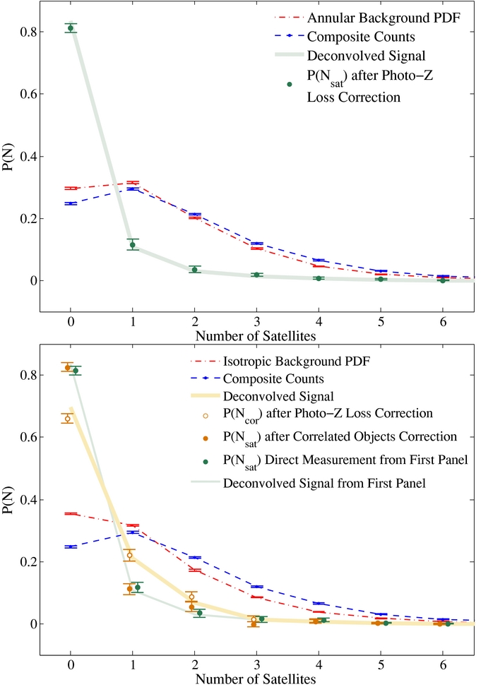
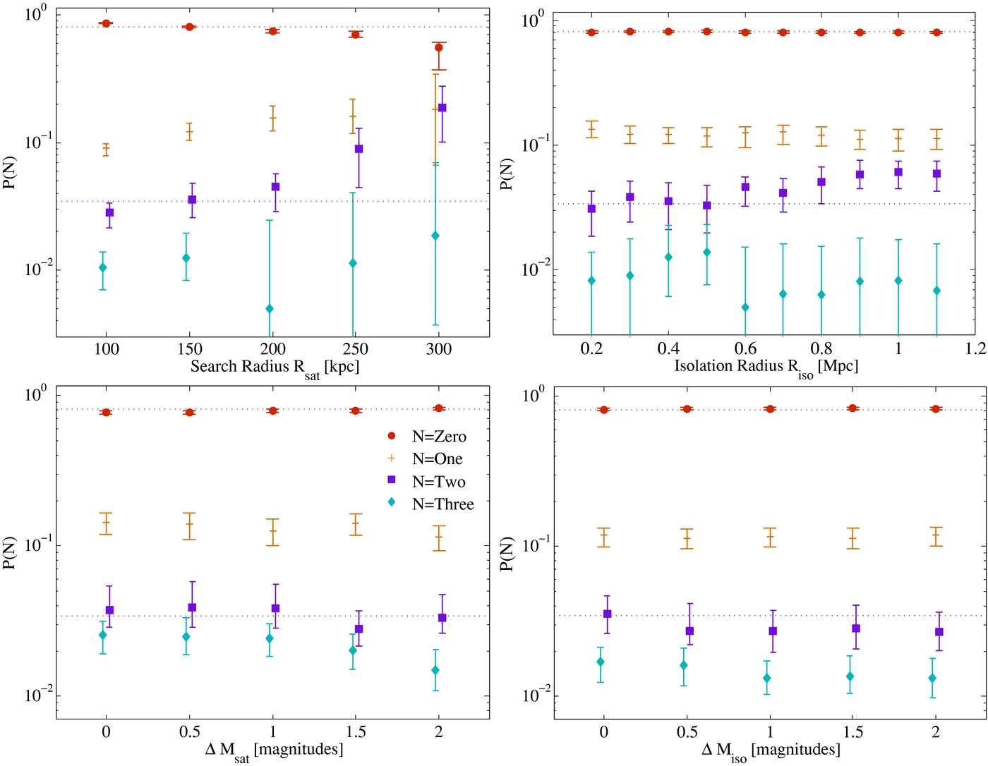
Figure 9. Probability of finding Ncor correlated objects around an MW analog in a cylinder with radius Rsat = 150 kpc, computed using three different data sets. Gray: results using hosts from the Northern Galactic Cap region of the SDSS spectroscopic main catalog and satellites from photometric main catalog. Blue: results using hosts from the Stripe 82 region of the spectroscopic catalog and satellites from photometric co-added data. Orange: results using hosts and satellites only from the NGC region of the spectroscopic main catalog.
Download figure:
Standard image High-resolution image
6. CONCLUSIONS
We have investigated the occurrence of dwarf satellites with luminosities similar to the Magellanic Clouds around host galaxies with environment and luminosity similar to the MW. Our analysis uses spectroscopic data from SDSS to identify isolated MW-like galaxies and then searches the SDSS photometric data for potential satellites between 2 and 4 mag fainter than these hosts. The primary result, summarized in Table 1 is the probability distribution of hosting Nsat satellites similar to the LMC and SMC. We find that, of our 22,581 MW-luminosity host galaxies, 81% have zero satellites as bright as the Magellanic Clouds, 11% have one such satellite, and only 3.5% host two such satellites.
The main source of uncertainty in our analysis is the presence of projected foreground and background objects along the line of sight to each MW analog. We correct for these in two stages. First, we reject most background objects with a rough photometric-redshift cut, and then we statistically correct for the remaining background objects by comparing the counts around MW analogs to counts in areas of the sky that do not contain MW-like objects. Because the background-noise level (rather than the sample size) is the dominant source of statistical uncertainty in our main analysis, the best potential for improving upon the precision of our results would come from an improvement in the photometric redshift estimates of faint objects, which would allow a more stringent initial background rejection.
The specific manner in which the background-estimation fields are selected has important implications for our final results. Fields chosen at random positions on the sky do not account for the clustering of galaxies, which will enhance line-of-sight projections around our chosen hosts, although an approximate correction can be calculated. We emphasize that such a correction is needed even when perfect spectroscopic information is available. Alternatively, the background fields may be chosen as annuli around each host, outside of the satellite search radius. This accounts for both random and correlated line-of-sight projections, and it is the technique we use for our main results. However, the optimum radius for these annuli is not entirely obvious, and this introduces a small additional systematic uncertainty into our results. Allowing for this systematic error, it is possible that the percentage of MW analogs that host two MC-analog satellites could be as high as ∼5% (see Table 1).
Nevertheless, the clear qualitative conclusion is that the presence of the LMC and SMC makes the MW quite unusual among the population of galaxies with similar luminosity. This is broadly in agreement with earlier observational studies that found ≲ 1 satellite on average around typical bright galaxies (Zaritsky et al. 1993; Lorrimer et al. 1994; Chen et al. 2006; James & Ivory 2011). In fact, when we compute the average number of satellites from our measured p(Nsat) distribution in Table 1, we find 〈Nsat〉 = 0.3, which is lower than the mean values reported in those studies. However, because previous authors considered a much wider range of host and satellite luminosities than we consider here, we do not expect more than qualitative agreement in any case. Similarly, we do not find a statistically significant difference in p(Nsat) for red versus blue galaxies, and this appears to be in conflict with the results of Lorrimer et al. (1994) and Chen (2008), who find that early-type galaxies host significantly more galaxies than late-types do. However, the broad range of host luminosities considered in those earlier studies, combined with the different luminosity distributions of early and late types, means that the underlying trend they found could be with luminosity, rather than color.
Our results are useful for understanding the larger cosmological context of the MW. There is a striking agreement between our results and the predictions of recent high-resolution cosmological N-body simulations. For example, Boylan-Kolchin et al. (2010) found that MW-sized dark matter halos hosted two MC-sized subhalos only ≲ 10% of the time in the Millennium II simulation (Boylan-Kolchin et al. 2009). Similar results are obtained with the Bolshoi simulation; the consistency between our results and the Bolshoi predictions will be discussed in detail by Busha et al. (2011b). This agreement constitutes an important confirmation of the cold dark matter paradigm for galaxy formation.
Our result also indicates that the MW is somewhat unusual among galaxies of similar luminosity at least in terms of its satellite population. A major philosophical underpinning of our cosmology is the Copernican principle, which holds that we do not observe the universe from any privileged position, except insofar as such a position is required for our existence (e.g., our very atypical position on a rocky planet with an atmosphere). Since there is no obvious anthropic requirement on the number of bright satellite companions to the MW, it would not be unreasonable to wonder whether our results present a challenge to the Copernican principle.
Applied to the expected properties of our home galaxy, a reasonable statement of the principle is that the MW should be consistent with a galaxy chosen at random from the stellar-mass-weighted galaxy population at large. It is important to note that this does not necessarily mean that the MW should be "typical" in all possible respects. In particular, it is not particularly unexpected that a randomly selected galaxy will be a ∼2σ outlier by at least one measure. Moreover, there is now reasonably strong evidence that the LMC and SMC were recently accreted by the MW and are on their first pass through the halo (e.g., Besla et al. 2007; Busha et al. 2011a). If this is true, then the presence of the Magellanic Clouds may be a transient event in the formation history of the MW, implying that the MW is not fundamentally unusual in any way. Thus, we may conclude that the unusually large population of bright satellites around the MW can likely be ascribed to happenstance and presents no special challenge to our basic cosmological paradigm.
This project has made use of data from the Sloan Digital Sky Survey (SDSS). Funding for the SDSS has been provided by the Alfred P. Sloan Foundation, the Participating Institutions, the National Aeronautics and Space Administration, the National Science Foundation, the U.S. Department of Energy, the Japanese Monbukagakusho, and the Max Planck Society. The SDSS Web site is http://www.sdss.org/.
The SDSS is managed by the Astrophysical Research Consortium (ARC) for the Participating Institutions. The Participating Institutions are The University of Chicago, Fermilab, the Institute for Advanced Study, the Japan Participation Group, The Johns Hopkins University, Los Alamos National Laboratory, the Max-Planck-Institute for Astronomy (MPIA), the Max-Planck-Institute for Astrophysics (MPA), New Mexico State University, University of Pittsburgh, Princeton University, the United States Naval Observatory, and the University of Washington.
We thank Marcelle Soares-Santos, Ribamar Reis, Huan Lin, and Jim Annis for providing us with the SDSS Stripe 82 co-add data and photometric redshifts in a usable form, as well as for providing the spectroscopic validation set for these data. We thank Carlos Cunha for several useful discussions about photometric redshifts and for providing photo-z's for the SDSS main sample. We thank Sarah Hansen for useful discussion about statistical background correction, Jeff Newman for helpful advice about correlation functions, and Marla Geha and Louie Strigari for useful input about the satellites of the Milky Way. The purity and completeness of our sample was tested using halos from the Bolshoi simulation. We thank Anatoly Klypin and Joel Primack for providing access to this simulation, which was using NASA Advanced Supercomputing resources at NASA Ames Research Center.
R.H.W., L.L., and M.T.B. were supported by the National Science Foundation under grant NSF AST-0807312; R.H.W., B.F.G., and P.S.B. received support from the U.S. Department of Energy under contract number DE-AC02-76SF00515.
Footnotes
- 4
Indeed, as we will discuss, even in the case of perfect spectroscopic information, redshift-space distortions lead to significant contamination from interlopers, which must be accounted for.
- 5
- 6
The superscripts indicate the assumed redshift to which the colors k-corrected; 0.1 is standard for the VAGC, while 0.0 is appropriate for the MW. We assume h = 0.7 in computing all k-corrected absolute magnitudes.
- 7
Although the MW and M31 are gravitationally bound, and M31 may be the more massive galaxy, the MW is not classified as a satellite of M31, since the two galaxies do not (yet) form a virialized system.
- 8
This happens occasionally, though infrequently, owing to fiber conflicts in the SDSS spectrograph.