An overview of SMath Suite
Published March 2015
•
Copyright © 2015 Morgan & Claypool Publishers
Pages 1-1 to 1-31
You need an eReader or compatible software to experience the benefits of the ePub3 file format.
Download complete PDF book or the ePub book

Permissions
Abstract
This chapter gives an overview of the SMath Suite.
Throughout the book reference is made to SMath files in the form [LinearRegress1.sm], generally at the start of a paragraph. All these files are available on the books website. Files with names ending with M, M1, etc. are functional only when opened with SMath with Maxima.
1.1. What is SMath Suite?
[Overview1.sm.] The developers of SMath Suite call it a mathematical program with paper-like interface and numerous computing features. SMath has many of the features found in the expensive application Mathcad but differs in that SMath is free. Some of its features are shown in figure 1.1. The SMath user interface resembles that of Mathcad.

Figure 1.1. The SMath interface.
Download figure:
Standard image High-resolution imageAlthough the application is correctly called SMath Suite, it is normal to use just the word SMath. However, when doing an internet search always use the full name to avoid hitting sites dealing with an unrelated item.
1.2. How do I get SMath Suite?
The website http://en.smath.info/ has downloadable files for a Windows and a Linux (Mono) installation. They are quite small: about 2 and 1 MB, respectively. The author has used SMath under Windows XP, 7 and 8.1.
At the site http://smath.info/wiki/SMath%20with%20Plugins.ashx one can obtain a Windows portable version. Just download the 78 MB Zip file and expand it to a USB thumb drive. Now you can run SMath on any computer without having to do an installation. This will appeal to students who wish to run it on a university computer for which they do not have installation privileges. This unofficial version has been greatly enhanced by Professor Martin Kraska (University of Applied Sciences, Germany) who has added the Maxima plug-in. These enhancements can be ignored when using examples from this book, but see chapter 10.
You can also run the 'cloud' version of SMath in your browser at http://smath.info/cloud/ but it is rather limited at the moment.
1.3. How can I get help with SMath?
The official SMath site is http://en.smath.info/. At the top of the page you will find links to a forum where questions can be asked and answered, and to a Wiki which gives access to tutorials, example, and helpful documents. Here is a good way to do a Google search: polyroots site: http://en.smath.info.
1.4. The SMath interface
As can be seen in figure 1.1, the SMath interface has a menu bar and a tool bar. Later we will see the SMath palettes. The work area on the interface is technically called a page, but you will also find it referred to as a worksheet. An SMath file holds one page.
The File and Edit menu items contain the controls one expects in such menu items in a Windows environment. File has Save, SaveAs, Print, etc while Edit has Cut, Copy and Paste, etc. All the normal keyboard shortcuts (e.g. Ctrl+S for Save, Ctrl+C for Copy) work in SMath. The other items on the menu bar are discussed as we proceed. The asterisk in Intro1.sm* on the title bar indicates the file has not been saved since it was last edited.
It should be noted that a file may be saved in its native format (note the extension sm) or as an image file (the default is png but the user can change the extension to jpg, bmp, or gif). There are other SaveAs options but we will look only at the executable file (exe)—see chapter 8.
While one can easily print an SMath file, a student using SMath for an assignment might save several SMath files as images and then insert them into a Word file. This will give more control over pagination, headers and footers etc.
The SMath Studio toolbar contains 21 icons (figure 1.2) which are briefly described below.

Figure 1.2. The SMath toolbar.
Download figure:
Standard image High-resolution image
| 1. New page | 11. Text color (of items to be entered) |
| 2. Open (existing worksheet) | 12. Background color (of items to be entered) |
| 3. Save (current worksheet) | 13. Control border (frames selected items) |
| 4. Print (current worksheet) | 14. Align horizontally selected items |
| 5. Cut | 15. Align vertically selected items |
| 6. Copy | 16. Function (insert a function) |
| 7. Paste | 17. Unit (insert unit) |
| 8. Undo (recent action) | 18. Reference book (see Help) |
| 9. Redo (recent action) | 19. Recalculate page |
| 10. Font size (of selected items on page) | 20. Interrupt process |
| 21. Show/hide side panel | |
Items (1) through (4) manipulate new or existing worksheets. Items (5) through (7) are well-known editing functions. Items (8) and (9) will undo and redo the most recent action. Items (10) through (12) adjust font or background properties—see Construction Regions below. Item (13) allows you to put a frame over an entry; for example, to show a solution to a problem. Items (14) and (15) re-align selected cells. Items (16) and (17) open the Function and Unit menus, which are also available in the Insert menu. Item (18) is also available under the Help menu. Items (19) and (20) are also available in the Calculation menu. Item (21) shows or hides all the palettes on the right-hand side of the page.
The palettes (figure 1.3) contain mathematical, graphical, and programming functions that can be placed in the main window. Each palette may be condensed or expanded on the tool on its header ⊡. The panel containing the palettes may be toggled on/off with the last item on the toolbar.

Figure 1.3. The palettes.
Download figure:
Standard image High-resolution imageWe will briefly explore some of these palettes and what they contain. Note that allowing the mouse pointer to hover over an item causes its name to be displayed.
As expected, the π tool inserts that symbol; this is one of SMath's numerical constants with the value 3.12.... The square roots tool is readily identified; the keyboard short cut is \. Similarly, one can see the multiplication operator × but most users will type *. In either case, SMath converts the operator to a middle dot, as in area:= width · length.
To assign a value to a variable or to define it in terms of other variables the definition/assignment operator := is used. This is the penultimate icon on the Arithmetic palette but normally the user types just a colon (:) and SMath converts it to the operator.
The Functions palette contains only a few of the functions available from Insert | Functions. The iconic tools for summation, product, differentiation, and integration are very useful.
Items in the Matrix and Programming palettes are discussed later.
The two Symbols palettes enable the user to insert Greek letters into a page. The alternative method is to type the Roman letter followed by Ctrl+G to convert it to Greek.
1.5. Constructing regions
There are two types of regions: text and math. In figure 1.1, the phrases Simple math, Root finding, etc are text regions while the assignment of a value for x (as in x:=5) is a math region. As you move the mouse around, you will see a red cross on the page; this is the insertion point and anything you type (or insert using a palette) will begin at that point. There are some exceptions for operators inserted from a palette. In addition to the two types of regions, it is possible to construct plots and to paste images onto an SMath page—figure 1.1 shows a plot and an inserted image. Note that SMath is 'top down' (you cannot refer to a variable before it is defined) so the plot of g(x) is about as high up the page as it can be.
The screen captures below may help you understand the comments in the next three paragraphs.

Download figure:
Standard imageTo make a text region either use the command Insert | Text Region or begin the text with a double quote which will not be recorded. If you just start typing some text, SMath will recognize it as a text region when you enter a space. As soon as this happens a small yellow box appears to indicate your language. To start a new line in a text region use Shift+Enter rather than just Enter.
Looking at the top line in figure 1.1 we see definitions for three variables (x, y and ans). Recall that we can begin the last one either by typing ans: or by typing ans and then clicking the definition operator (:=) in the Arithmetic palette; in each case we have a partial definition with a place holder. Again we have two options: (a) we could enter the numerator (x − y)2, then the division operator and type the denominator x, or (b) use the division operator to give the template shown here and then add the numerator and denominator. The trick in constructing and editing formulas is to watch the poistion of the insertion symbols ⌊ and ⌋. Once a variable has been defined it will appear in the dynamic assistant. So if we begin to type an we will see the definition for ans.
To copy, move or align one or more regions begin by clicking to one side of a region and then drag the mouse to select all the required regions. Use the Ctrl key to select non-adjacent regions. When the mouse button is released just the regions are shown as selected. Now you can drag to a new position, use one of the alignment tools or issue the Copy command (Ctlr+C is the easiest way). The same selection method can be used to give one or more regions a border, a background colour or a different font size. A region selected in this manner can be copied by holding down the Ctrl key as you drag the region. Text regions can be made bold, underlined and/or italicizied—these effects will apply to the entire text; one cannot enhance just part of a text region. Do not confuse the selection method here with clicking and dragging inside a region to make it dark blue.
1.6. Greek characters
Greek characters (for use in text or math entries) may be entered either: (a) by clicking on the appropriate symbol in the palette, or (b) by typing the Roman letter (see table 1.1) followed by Ctrl+G. Thus D followed by Ctrl+G gives Δ. The symbol π (pi) may be inserted as p followed by Ctrl+G; from the symbol or arithmetic palette, or with Ctrl+Shift+p. When inserted into a math area π (pi) will have the value 3.14 159 265....
Table 1.1. The Greek alphabet.
| Lower case | Upper case | Name | Roman letter | Lower case | Upper case | Name | Roman letter |
|---|---|---|---|---|---|---|---|
| α | Α | alpha | a | ν | Ν | nu | n |
| β | Β | beta | b | ξ | Ξ | xi | x |
| γ | Γ | gamma | g | o | Ο | omicron | o |
| δ | Δ | delta | d | π | Π | pi | p |
| ε | Ε | epsilon | e | ρ | Ρ | rho | r |
| ζ | Ζ | zeta | z | σ | Σ | sigma | s |
| η | Η | eta | h | τ | Τ | tau | t |
| θ | Θ | theta | q | υ | Υ | upsilon | u |
| ι | Ι | iota | i | ϕ | Φ | phi | f |
| κ | Κ | kappa | k | ψ | Π | psi | y |
| λ | Λ | lambda | l | χ | Χ | chi | c |
| μ | Μ | mu | m | ω | Ω | omega | w |
The reader may wish to skim through the rest of this chapter and return to it when using a particular SMath feature.
1.7. Option settings
The Tool menu item has an Options item which leads to the dialog shown in figure 1.4. Most of these are self-explanatory. All these settings apply to the entire page and will be used next time the user starts SMath. We have seen that a text region can be individually formatted. The decimal and exponential threshold setting for a math region displaying a number can also be altered on an individual basis. Suppose, with the decimal places set to 8 and exponential threshold at 5, we see on a page x = 128.22 827 158. We can select the region by left clicking, then by right clicking bring up a menu from which Decimal places may be chosen; this leads to the dialog in figure 1.5. The process can be repeated to change the exponential threshold to 1. Now we have x = 1.282×10² .

Figure 1.4. The Options dialogs.
Download figure:
Standard image High-resolution image
Figure 1.5. Change the decimal setting for one region.
Download figure:
Standard image High-resolution image1.8. Scratchpad calculations
The reader is encouraged to treat this section as an exercise by typing what is shown in the left hand column on a new SMath page, observing the movement of the insertions symbol ⌋ and to see why the results in the right hand column are obtained. The symbol → is used to denote the right arrow key or the spacebar.
| 1 + 5/6 + 7/8 | |
| 1 + 5/6→ + 7/8 | |
| On the SMath page, left click the result above, then right click and select Fractions followed by Fractions. | |
| See if you can get the first result rather than the second. |

1.9. Simple algebraic calculations
It must be emphasised that SMath is case sensitive. So a variable defined as v and another as V are totally different items. The reader is advised not to use π or e as variable names as these are defined in SMath as mathematical constants—see below. Also it is recommended not use the single letter i for a variable name but to reserve its use for the imaginary number √−1. The use of the single letter l is discouraged as it is easily confused for the digit 1.
[Overview2.sm.] Figure 1.6 shows an SMath page with some simple definition and display math regions. As a warm up to delving deeper into SMath, the reader is invited to recreate such a page, perhaps with the explanatory text omitted. Note how typing a: results in a:=. When you type c:a*b, the conversion to c := a·b is instantaneous.

Figure 1.6. Some simple math operations.
Download figure:
Standard image High-resolution imageExperimentation is encouraged:
- 1.Change the global decimal place setting and the decimal setting for an individual region.
- 2.Can d be displayed as a fraction?
- 3.Find other ways to obtain the √ operator.
- 4.Have you mastered the two alignment tools?
- 5.When you drag the d = 0.8 region up the page it becomes d = ▪ with a red border; why?
- 6.Is there another way to compose the x assignment?
- 7.Can you change the value of b without retyping the entire assignment?
- 8.Click on z = 4.79 then right click and from the popup menu use Optimization | Symbolic.
- 9.Experiment with unchecking the AutoCalculation in the Calculations menu item. Then change the value of a. Does anything happen to the other displayed values? What does F9 do? Remember to put AutoCalculation back on.
- 10.Type z→ using the arrow in the Arithmetic palette. This tells SMath to use symbolic representation. Note that the arrow becomes =. Some documents on the SMath website show the arrow being displayed but this has been changed in the newer version of SMath.
- 11.The √ symbol in the text region was pasted from a Word document. Try copying some math regions from the SMath page to a Word document; here is an example z:sqrt(a^2−b/2).
1.10. Subscripted variables
It is convenient in many problems to use variable names such as x1 and x2 to emphasize their similarities. To achieve x1:=3 the user types x [dot] 1:3 where [dot] indicates the period (full stop) key. Later in this chapter we will discuss indexed variables—elements of vectors and matrices. These are constructed in a different manner and (if one looks close enough) have a slightly different appearance.
1.11. Working with units
[Overview3.sm.] This topic will be demonstrated with a simple hydrostatics problem. Water is pumped at a constant rate r = 6 m3 min−1 through a pipe. The pipe diameter near the pump is 20 cm but this widens to 40 cm at the end. Find the velocity of the water at the discharge point. We reason that, since water is incompressible, the rate of flow at any point in the pipework is constant. So r = v1 ·A1 = v2 ·A2 where v is the velocity and A the cross-sectional area. Figure 1.7 shows the page for this calculation.

Figure 1.7. Example of a calculation with units.
Download figure:
Standard image High-resolution imageThere are several way of entering units. Method (a): suppose we have typed d1:=20 and the region is still active. From the menu bar use Insert | Units to bring up the dialog shown in figure 1.8. Note how the left panel shows various categories but we have selected All. In the Quick box we entered meter (note the US spelling). Now in the right hand panel we can select centimeter (cm) and click the Insert button, or we can double click the cm entry in the dialog. In either case the dynamic assistant pops up so we tap the Tab key to confirm we want this unit. Method (b): now we have typed d2 := 40 and wish to add the cm unit. We type a single quote (') and this causes the units menu to pop up; we type cm and this locates the desired unit and we confirm with the Tab key. Note that when the user types the single quote, SMath adds a place holder but it is more oval than the normal rectangular place holder.

Figure 1.8. The Units dialog.
Download figure:
Standard image High-resolution image
Download figure:
Standard imageThe progression to get r := 6 m3 min−1 is: after typing r : 6, insert the m unit and then use ^3. Now insert the min unit and use ^−1. While units are shown in blue, any exponent for a unit is not.
Note how SMath looks after unit conversion. We have centimetres and minutes in the data but the result show metres and seconds. SMath always shows standard SI units in numerical evaluation regions. However, as seen in figure 1.7, we can override this. Click on a region displaying v2 := 0.8 m, use the right arrow key to get to the far right of the region, and then use the single quote to indicate that you wish to add units, and add the required units. If you enter inappropriate units, the regions will show no numeric value and will have a red border.
1.12. Physical and mathematical constants
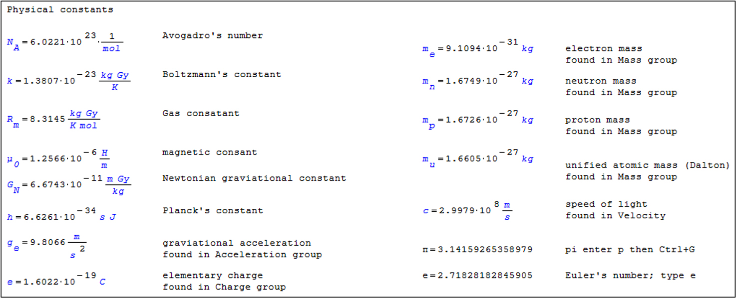
[PhyConst.sm.] SMath has a number of built-in physical constants and two mathematical constants (π and e). These are shown in figure 1.9. All of the physical constants are to be found using the same techniques as adding a unit. In the left panel of the units dialog (figure 1.8) there is a group called Physical Constants within which the first six physical constants may be found. The others are in groups as shown in the figure. Of course, the All group contains every one.

Figure 1.9. SMath's physical and mathematical constants.
Download figure:
Standard image High-resolution imageClearly, the current version of SMath has trouble displaying the correct units for Boltzmann's k, the gas constant Rm, and the Newtonian gravitation constant GN. However, SMath 'knows' the correct units and displays them in the dynamic assistant and uses them in calculations.
To insert a physical constant symbol into a math region use the same techniques as for unit. So to get the region shown to the right, after typing the 2, the user typed ' (single quote to indicate a unit is needed), g to locate the items beginning with g, a period to indicate a subscript in preparation for typing an e. As it turns out, there was no need to add the e since the dynamic assistant located ge. All that remained was to tap the Tab key to confirm the choice.

Download figure:
Standard imageIf you use π or e in a formula without assigning a value then the values shown in figure 1.9 are used. If values are assigned, they will override the built-in values. It is recommended that values not be assigned to either π or e.
1.13. SMath functions
SMath contains a large number of predefined, or intrinsic, functions for both real and imaginary numbers. We will not discuss the last group. The complete list of functions can be found in Appendix A. The entire collection of functions is accessible from the Insert Function dialog (figure 1.10) which is accessed by the menu command Insert | Function or by clicking the f(x) tool. It is worth noting that the dialog provides a brief description and syntax for a selected function. An alternative way of inserting a function is to type the function name (or part thereof) and let dynamic assistant help you to get it right.

Figure 1.10. The Insert Function dialog.
Download figure:
Standard image High-resolution image
Download figure:
Standard imageA user wishes to define x with x := 2·ln(z). Method (a): after typing 2*, he clicks the f(x) tool, locates the ln function in the Insert Function dialog, which he double clicks, or he clicks the Insert button. Unfortunately, the Insert Function dialog has no Quick Search facility, so you must scroll all the way through. The task is shorter if you correctly guess what group to use from the left panel. Now he has the template shown above.
Alternatively, since he knows the name of the function, after typing the 2* he types ln and up pops the dynamic assistant. He commits his choice with the Tab key. Note that in the dynamic assistant functions are shown in purple while units are blue.
1.14. Matrices and vectors
[MatrixMath.sm.] A matrix is constructed by clicking the first icon in the Matrix palette or by using the shortcut Ctrl+M. This bring up a dialog where one specifies the number of rows and columns; following this the matrix elements are entered into the place holders. The sequence is shown in figure 1.11. A vector is constructed in the same way, i.e. as a one column matrix.

Figure 1.11. Constructing a matrix.
Download figure:
Standard image High-resolution imageAn alternative way of constructing a matrix is to type A:mat, which generates a 2 by 2 matrix template. By clicking on either of the matrix brackets one can have SMath present a fill handle in the lower right corner; dragging this can expand the rows and/or columns to the required number.
At the bottom of figure 1.11 we see how to reference a matrix element: type A [3, 2 = to make this math region. Note the use of [ to get an index compared to [period] to get a subscript. There is more white space between the matrix name (A) and the first index (3) than there would be if we had a variable A with a subscripted 3.
Some simple matrix math is demonstrated in figure 1.12. In a later chapter we see how to use matrix math to solve a system of equations.

Figure 1.12. Examples of matrix math.
Download figure:
Standard image High-resolution image[Vector.sm.] The range functions may be used to generate vectors with numerical elements as seen in figure 1.13. Coupling this with the augment function we can define a matrix—see figure 1.14.
- •range(start, end): shows up in the worksheet as start..end, and produces a vector whose elements are start, start+1, start+2, ... end.
- •range(start, end, start + increment): shows up in the worksheet as start, start + increment ... end, and produces a vectors whose elements are start, start + increment, start + 2 increment, etc. The last element is the lowest value smaller than end by less than increment.

Figure 1.13. Using the range functions to define a vector.
Download figure:
Standard image High-resolution image
Figure 1.14. Using augment to make a matrix.
Download figure:
Standard image High-resolution imageThe cross product of two three-element vectors (X and Y) is found with C:= X × Y, where the × operator is the last item on the Matrix palette.

[VectorMath.sm.] SMath has problems with symbolic evaluation of vector math and incorrectly applies the scalar rules for commutation and distribution. If in doubt, use numerical optimization with vectors and matrices.
1.15. Drawing graphs
SMath has limited graphing facilities; they are useful only for personal work or, at a pinch, for internal reports, but not for publication work. SMath can generate two- and three-dimensional graphs. We will explore only the 2D graphs. For more information on graphing see http://smath.info/wiki/Graphs.ashx.
In section 10.2 there are notes on the XY Plot function in SMath with Maxima.
[Graph1.sm.] We begin with a very simple example: a plot of a cubic function—see figure 1.15.
- 1.Click on the point in your worksheet where the upper left corner of graph will go.
- 2.Use the Insert | Plot | 2D menu option. Alternatively, use the keyboard shortcut of typing @.
- 3.Type the function x^3 − 6*x^2 + 11*x−6 in the place holder in the lower left corner of the graph.
- 4.Use the mouse wheel to rescale both axes. Drag the centre of the plot to keep the zone of interest (where we see the three roots) visible.
- 5.Resize the plot by dragging one of its fill handles.

Figure 1.15. Plotting a function of x.
Download figure:
Standard image High-resolution imageWhen using this method, we must use a function of x; no other variable name will work. Furthermore, we have no control over the range of x-values; we address this in later chapters.
The methods for modifying a graph are listed below; you must first 'activate the graph' by clicking on the graph so that the handles are displayed:
- 1.Drag one of the handles (small solid squares) to resize the graph.
- 2.Drag the mouse pointer to reposition the origin.
- 3.Scroll the mouse wheel to rescale both axes.
- 4.Scroll the mouse wheel while holding down CTRL to rescale the y-axis.
- 5.Scroll the mouse wheel while holding down SHIFT to rescale the x-axis.
Sometimes when you plot a function the graph appears empty. In such cases it is necessary to rescale the graph to find the plotted data. Try plotting x2 + 75x − 2500; you will see nothing until the x scale is about ±64 and the y scale ±1024.
At the time of writing, SMath (version 0.97.5346) has a problem with certain high resolution Microsoft wireless mice (model 4000, for example). The plot scales increase regardless of the direction of rotation of the wheel. A fix for this problem is planned.
To relocate the graph on the page: click outside the graph and drag the mouse until the graph is selected (blue background with default setting); now drag it to new position. To copy or delete a graph you need to select it in the same way. Alternatively, a graph (or any region) can be moved by dragging it by the outside frame when the mouse pointer is a four-pointed arrow.
[Graph2.sm.] Two or more functions can be plotted on one graph (figure 1.16) by using the multiple values tool—it is the last one in the Functions palette. What is produced is sometimes called a list. The list may be external to the graph or used in the graph place holder. When you click on the tool a template with two place holders is displayed. To add more items to the list, click on the brace { and drag the resulting fill handle (lower right corner) down. Items can be deleted by dragging it up.

Download figure:
Standard image High-resolution image
Figure 1.16. Plot of two functions.
Download figure:
Standard image High-resolution image[Graph3.sm.] Figure 1.17 has five functions plotted and gives some idea of the colours used by SMath with blue being used for the first function.

Figure 1.17. Plot to show colours used by SMath.
Download figure:
Standard image High-resolution image[Graph4.sm.] Figure 1.18 demonstrates how to add text and points to a graph. The variable plottext is a 2×5 matrix: the first two elements in a row specify the starting position (x, y), then the text to be displayed, followed by the font size and colour. Similarly, in each row of the 7×5 matrix Points we have: x-position, y-position, symbol, font size, and colour. See the note below regarding the symbol.

Figure 1.18. Adding texts and points to a graph.
Download figure:
Standard image High-resolution imageSMath offers over 140 colour choices from aliceblue to black—see http://en.smath.info/forum/default.aspx?g=posts&m=3663. A misspelled colour name will result in black being used. It is not possible to type the = symbol within a text element in a vector; the = symbol in y = mx + b was produced with Alt+205.
[Graph5.sm.] The plotG function, which was made available by Professor Radovan Omorjan in the SMath Studio forum, is illustrated in figure 1.19. The program takes vectors of values (x, y) and creates a plot matrix for the data using a specified character (char), size, and colour. The plotG function saves us the work of making a matrix similar to Points used in the previous example. The vectors x and y could represent experimental data and yline is the equation of linear best fit. The syntax for using this is Variable := plotG(xdata, ydata, char, size, colour); then Variable is used in one of the plot place holders. The reader may wish to experiment with different characters, sizes and colours.
For the value of char, use only one of: the period character which displays as a solid circle; the lower case character o which displays as a circle; x which displays as a cross; the asterisk (*) which displays as a star. Other characters are plotted incorrectly—too low and too far to the right.

Figure 1.19. The plotG function.
Download figure:
Standard image High-resolution imageIt is suggested that you copy and paste the plotG function from the file Graph_PlotG.sm rather than try to code it. Also refer to section 1.19 to see how to make a snippet to allow the plotG function more readily accessable.
[Graph.sm.] If we have a function such as f(x) defined on an SMath page and enter f(x) in the plot's place holder, then we have no control over the domain used by the plot. This can be rectified using the augment function. This method is explained in figure 1.20.

Figure 1.20. Using the augment function to plot.
Download figure:
Standard image High-resolution image1.16. Solving equations and finding roots
When we speak of solving an equation we mean finding the value(s) of x that satisfy the equation f(x) = g(x). For example we might wish to know what value of x gives the function exp(x2 + x) the value of 10. When we speak of finding the roots of f(x), or finding the zeros, we mean finding what values of x makes f(x) = 0.
[Quadratic.sm.] We will start this topic by finding the roots of a simple quadratic equation. In figure 1.21 the bordered text box shows the equation whose roots we seek, but the expression is not used in the calculation; rather we use the values of the coefficients a, b and c as entered in the first row. The familiar quadratic equation is entered; observe the ± which is obtained from the Arithmetic palette. Since, in general, a quadratic has two roots, when x= is used to display the roots then multiple values (a list) result. The figure shows that plugging each value into the second order equation gives the result zero, proving we have the roots; note that an element in a list is referenced in the same way as in a vector—using an index not a subscript. So to display the value of x1 we type x[1=; note how on the SMath page there is white space between the x and the 1, denoting an index.

Figure 1.21. Finding roots of a quadratic equation.
Download figure:
Standard image High-resolution imageBy changing just the values of a, b and c, the reader might wish to find the roots of 9x2 + 12x + 4 and x2 − 9 to see what happens when there is one root, and 3x2 + 4x + 4 which has a negative discriminate and hence has imaginary roots.
[Polyroots.sm.] The polyroots function is demonstrated in figure 1.22 where the roots of a quadratic (x2 + 3x − 18) and of a quartic function (x4 − 15x2 + 10x + 24) are found. In the first example the user typed rootsA:=polyroots to make the template polyroots (▪). Then the place holder was converted to a vector (Ctrl+M brings up the required dialog and a 3×1 matrix—a vector—was specified) and the coefficients of the equation were entered starting with the coefficient for x° (i.e. the constant). The results are presented in vector form. Of course, we get the same roots as before for this quadratic. In the second example, a vector was made first and this was referenced in the polyroots template. The fourth element in coeff is zero since the quartic of interest has no x3 term. It was simpler to define a function to show the correct roots had been obtained.

Figure 1.22. Demonstrating the use of the polyroots function.
Download figure:
Standard image High-resolution imageThe polyroots function uses an analytical method to generate results that are accurate to within the precision of SMath (15 decimal places). The next two functions we will look at, roots and solve, use numerical approximation methods. The reader may be familiar with methods such as Newton–Raphson, secant, bisection, etc; a concise review of numerical methods can be found at http://www.maths.dit.ie/~dmackey/lectures/Roots.pdf.
[Roots.sm.] Normally we would use polyroots to find the roots of any polynomial but for the sake of comparison in figure 1.23 we use polyroots, roots and solve to get the roots of the cubic equation x3 − 2x2 − 3. The polyroots function finds three roots, only one of which is real. The functions roots and solve give only real roots.

Figure 1.23. Comparing polyroots, roots and solve.
Download figure:
Standard image High-resolution imageThe syntax of roots is either roots(argument-1, argument-2) or roots(argument-1, argument-2, argument-3), where each argument is either a variable or each is a vector. Our example uses variables with f(x) as the function whose roots are sought, x the variable to find, and, in the second and third cases, we have a number (3) to give roots a guess at the root. Our f(x) has only one real root but had there been three, the results would have been displayed in vector form, as we see below.
Looking at the first and second examples of roots it is clear why one is always encouraged to provide a guess—i.e. to use the three-argument form.
The third example, with _x rather than a simple x, is there to demonstrate a very important point. Figure 1.24 shows what happens when the second argument has been given a numerical value prior to being used within root. The calculation in the second example fails but the third example still works. The reader is encouraged to experiment. If you delete x := 2, you may need to press F9 to recalculate the SMath page. So why _x? Many SMath users employ a variable like _x rather than x in a roots evaluation since it is unlikely that such a variable will have been used before in the page. Others employ a variable similar to #x. You will see both in examples on the SMath website.

Figure 1.24. The roots function fails when argument-2 already has a numerical value.
Download figure:
Standard image High-resolution imageThe second argument in a roots evaluation cannot have been given a numerical value in any statement prior to the roots calculation.
[Roots2.sm.] Figure 1.25 demonstrates another example of the use of roots: to find the roots of a transcendental equation.

Figure 1.25. Finding the roots of a transcendental equation.
Download figure:
Standard image High-resolution image[Roots3.sm.] Figure 1.26 demonstrates the use of roots to solve a system of linear equations. In the upper part, the vectors are used for the three arguments; in the lower part the vectors are defined beforehand and are referenced by the arguments. In a later chapter we see how matrix math can be used to solve a system of equations.

Figure 1.26. Solving a system of linear equations.
Download figure:
Standard image High-resolution image[Roots4.sm.] Unlike the matrix method, the roots function method allows us to tackle systems of nonlinear equations, as shown in figure 1.27.

Figure 1.27. Solving a system of nonlinear equations.
Download figure:
Standard image High-resolution image[Solve1.sm.] In figure 1.28 the solve function is used to find the roots of the same function that was solved with the roots function in figure 1.25. Solve has the advantage of locating all the real roots in one operation and returning them in a vector. In the top part of figure 1.26 solve is used in the two-argument form solve(function-to-solve, variable). In the lower part we have the four-argument form solve(function-to-solve, variable, lower-limit, upper-limit).

Figure 1.28. Finding roots with the solve function.
Download figure:
Standard image High-resolution image[Solve2.sm.] The two-argument form of the solve function is sensitive to the last setting in Tool | Options | Calculate (see figure 1.4). This is demonstrated in figure 1.29. Normally a polynomial is best solved with polyroots but the quadratic here serves as a convenient example to make the point being made.

Figure 1.29. Solve response to the roots range setting.
Download figure:
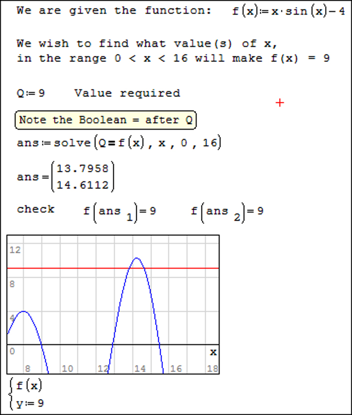
Standard image High-resolution image[Solve3.sm.] So far we have been finding roots, i.e. we have found x such that f(x) = 0. In the next example (figure 1.30) we see how to find x such that f(x) = Q where Q is some numerical value. A Boolean = must be used in the expression within solve.

Figure 1.30. Solving for a non-zero value of f(x).
Download figure:
Standard image High-resolution imageThings to remember when using the solve function:
- 1.The solve function cannot be used with units of measurement.
- 2.If the statement is enclosed in a red border and the message 'No real roots' appears when the mouse point hovers over the statement, then the user should experiment with various values for the third and fourth arguments—the lower and upper values of the range in which a root is sort.
- 3.When the first argument is an equation (e.g Q = f(x)) it is imperative that the equal sign be inserted from the Boolean palette.
1.17. Symbolic differentiation
[SymbolicDiff.sm.] The more advanced applications like Mathematica, Maple, MathLab, etc can perform various symbolic manipulations. SMath is limited to being able to do symbolic differentiation. Some examples are shown in figure 1.31.

Figure 1.31. Examples of symbolic differentiation.
Download figure:
Standard image High-resolution imageThe first-order differential template is found on the Function palette or can be generated by typing diff and accepting diff(1) from the dynamic assistant. The second-order template is generated by typing diff and accepting diff(2) from the dynamic assistant.
The → tool on the Arithmetic palette is used rather than the = from the keyboard to specify symbolic evaluation; the shortcut is Ctr+period. An earlier version of SMath displayed the → symbol rather than the = symbol but the current version converts it. Recall that if a math region is right clicked and the Optimization item is selected, the user can specify the type of evaluation.
It is to be hoped that every physics student is familiar with www.wolframalpha.com and its free mathematics services—see figure 1.32.

Figure 1.32. A sample from Wolframalpha.com.
Download figure:
Standard image High-resolution image1.18. Programming
Computer scientists speak of programs being constructed from three structures: sequential, branching (aka decision or conditional), and looping. In a sequential structure each statement is executed one after the other; in SMath this means from left to right and from top to bottom. SMath has one way to make a branching construct and that is the If...Else. SMath does not have the case construct found in many computer languages. There are two looping constructs: for and while. The for construct is used when one knows how many times some code is to be repeated; the while construct is used to loop until some condition is met.
1.18.1. The If...Else structure
[IfElse.sm.] Figure 1.33 illustrates an If...Else construct. The template is generated either by clicking if in the Programming or by typing if and accepting the construct from the dynamic assistant. There may be occasions when nothing is to be done in the else area. One option is to enter a 'O' but the word "continue" in quotes is more meaningful. Do not use the continue item from the programming palette.

Download figure:
Standard image
Figure 1.33. An example of the If...Else structure.
Download figure:
Standard image High-resolution imageVery often we need more than one statement to be executed after the If test or the Else condition. We can get this using the line command from the Programming palette. The sequence is shown below.
- 1.Start with the basic template; fill in the first place holder.
- 2.Click on the inner place holder—the second or the third.
- 3.Click on line in the Programming palette.
- 4.Click on the line to reveal a fill handle in the lower right area.
- 5.Drag this down as far as needed; drag up if you go too far.
1.18.2. The For structure
[CubeAddition.sm.] Figure 1.34 shows an SMath page which (a) sums the cubes of the first 12 integers, and (b) sums the cubes of the even numbers up to 12. The second part is done with two forms of the ranges in the for construct. We also see that SMath has a summation tool that makes all the work in (a) unnecessary!

Figure 1.34. Examples of for loops.
Download figure:
Standard image High-resolution image| for j ∈ 1..12 | Means vary j from 1 to 12 in increments of 1. |
| j∈ 2, 4..12, | Means start with j = 2, increment by 2 (since the difference in the first and second arguments is 2, i.e. 4 − 2 = 2) while j is less than or equal to 12. |
| j= 2,j ⩽ 12,j:= j + 2 | Means start with j = 2, and while j is less than 12, increment j by 2. NOTE: you must use the Boolean = in j = 2. |

Download figure:
Standard imageThe second and third constructs are equivalent, but the author finds the meaning of the third one to be clearer.
In these constructs, j is referred to as the loop variable. Programmers take great care never to explicitly change the value of a loop variable other than in the opening code of the for loop.
[CubeAddition.sm.] There is another variation of the for structure that uses no loop counter. It is used only in conjunction with vectors and matrices. Figure 1.35 shows an example: again we are summing the cubes of the even numbers from 2 to 12. The code for elem ∈ V may be thought of as 'for every element in vector V'. The name elem is unimportant, any valid name may be used.

Figure 1.35. Example of the for-every-element.
Download figure:
Standard image High-resolution image1.18.3. The While structure
[CubeAddition.sm.] Figure 1.36 shows an SMath page using while loops to sum the cubes of the natural numbers but not to exceed 1000. Clearly in the left hand side, the sum was exceeded. Indeed it could not have been otherwise since the test (sume ⩽ 1000) only fails when the sum exceeds the limit. So the programmer had to subtract the last j3. This is avoided in the code to the right where we have an if constructed nested within the while. Note the use of break to exit the loop.

Figure 1.36. Examples of while loops.
Download figure:
Standard image High-resolution imageWhen coding a while loop is it easy to make a mistake that causes the loop to run for ever—the exit condition is never satisfied. You will see a green border around the code that is being executed and the timer in the status bar keeps increasing. Press the Esc button and accept the invitation to cancel the calculation!
While you are working in a program structure, be careful to avoid typing the evaluation operator (=) when a definition operator (:=) is required. This mistake will result in egregious place holders in the top right corner of the structure and only after patient work with the delete, backspace and arrows keys will you have workable code.
1.19. Snippets
It may be helpful when a user finds he is repeating a particular piece of code in many worksheets, to place this code in a snippet. When SMath Studio is installed there are already two snippets available. These allow the user to readily work in degrees or in grads rather than in radians. In figure 1.37 the top part shows the calculation of some trigonometry functions; the last item in each row was given the symbolic optimization—either type = and then by right clicking the region, set the optimization to symbolic, or use the shortcut Ctrl+period in place of the =.

Figure 1.37. Using the Degrees snippet.
Download figure:
Standard image High-resolution imageIn the centre of the page there is a line with the notation Evaluation in Degrees, and under that some more calculations but this time with arguments in degrees not radians. Clicking the ⊞ at the left of the line will reveal the code that allows for this. To add the hidden code to the worksheet, click the place where the code is to added (look for the red cross), open the dialog shown in figure 1.38 using the command Tools | Snippet Manger, then double click the required snippet.

Figure 1.38. The Snippet Manager dialog.
Download figure:
Standard image High-resolution imageThe reader may be wondering how code gets added to the Snippet Manager. The process is relatively easy; here is a concrete example for a user wishing to add the plotG function as a snippet (figure 1.39).
- a)Open a file with the function; Graph_PlotG.sm for example.
- b)Copy and paste just the plotG function to a new page.
- c)Save the new file as plotG.sm on the desktop, and close SMath Studio.
- d)Using Windows Explorer (aka File Manager) move the new file from the desktop to the folder C:\Progam Files (X86)\SMath Studio\snippets.
Windows will prevent the user who attempts in step (c) to save directly to the snippet folder, hence the workaround of first saving it elsewhere. For those with the portable version of SMath Studio a direct save is recommended.
[SnippetExample2.sm.] The steps to use the new snippet are the same as before. The advantage of having the plotG snippet is being able to find the code quickly and make tidy worksheets where the plotG function is hidden and therefore is not obtrusive.

Figure 1.39. plotG used with a snippet.
Download figure:
Standard image High-resolution imageAppendix A. SMath functions

Download figure:
Standard image High-resolution image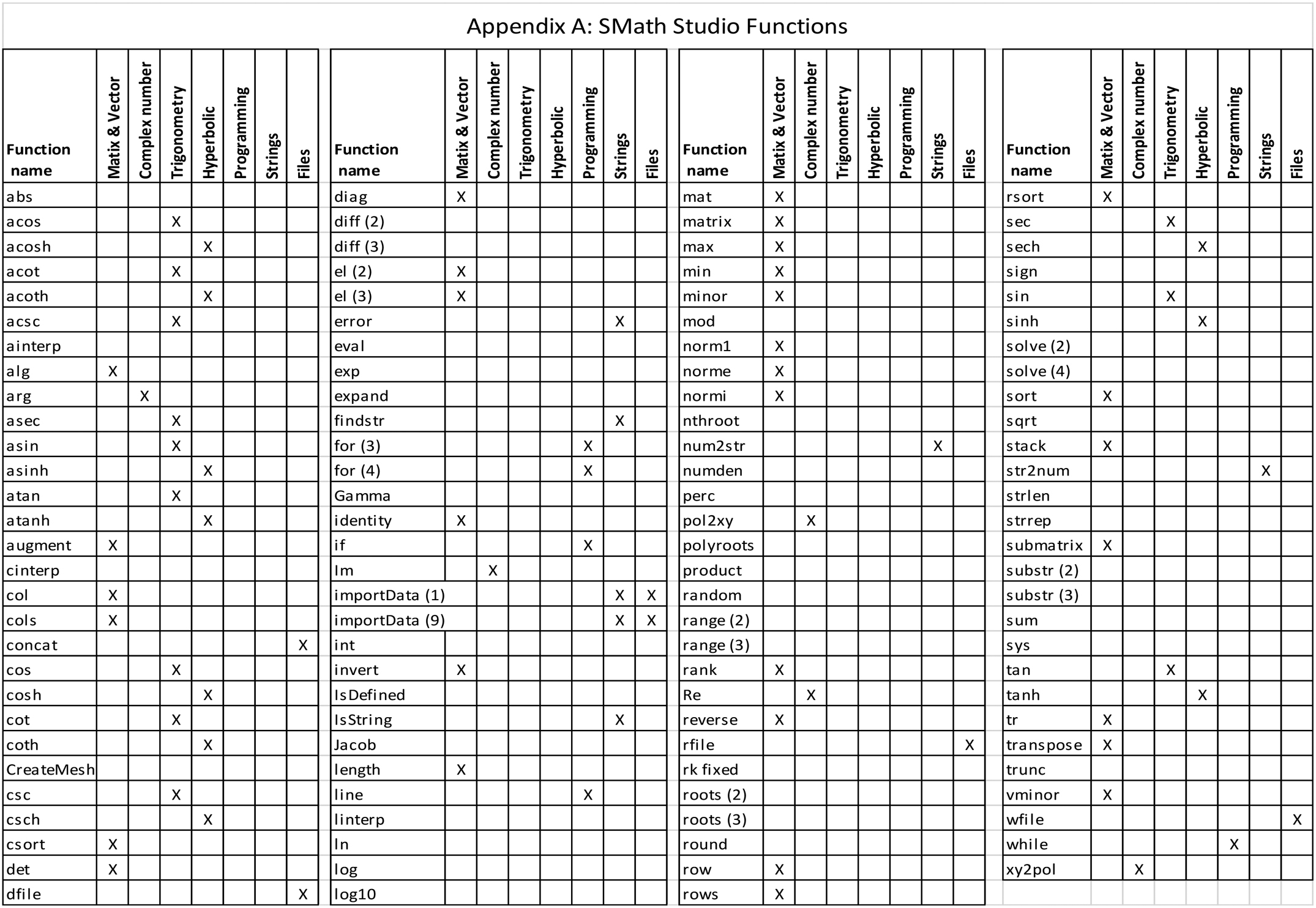