
Fluidic homogeneous continuous dynamical systems as fluidic commutation matrixers
Published December 2016
•
Copyright © IOP Publishing Ltd 2016
Pages 13-1 to 13-6
You need an eReader or compatible software to experience the benefits of the ePub3 file format.
Download complete PDF book, the ePub book or the Kindle book

Permissions
Abstract
This chapter describes fluidic homogeneous continuous dynamical systems as fluidic commutation matrixers.
Windmills, which are used in the great plains of Holland and North Germany to supply the want of falling water, afford another instance of the action of velocity. The sails are driven by air in motion—by wind.
Hermann von Helmholtz
13.1. Fluidic-transmission line
Let us consider one of the basic fluidic commutation matrixer components—the fluidic-transmission line. Figure 13.1(a) shows a mechano-fluidic (MF) pump.
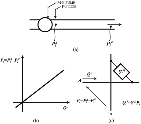
Figure 13.1. Fluidic-transmission line fluidic-commutation matrixer component.
Download figure:
Standard image High-resolution imageHow are we to describe this physical commutation matrixer component mathematically? To answer this question we must first decide what we wish to know about the passage of the fluid to a transmission line. One thing we want to know is the rate at which liquid is passing through the fluidic-transmission line. We call this the flow, and for a fluidic-commutation matrixer, it is designated as q. Another thing we might need to know is the size of the MF pump required to produce the flow. Instead of physical size, the pressure often indicates the capability of an MF pump, pA , it can develop.
If we were able to relate the pressure, pA, , to the flow, q, we would have a type of mathematical model of the fluidic transmission line. But can we do this? We cannot, because the flow through the fluidic-transmission line also depends on the pressure, pa , at the end of the fluidic-transmission line.
If pa were equal to pA , there would be no flow through the fluidic-transmission line. Thus the mathematical model must relate the flow, q, to the pressure difference, pA – pa .
These quantities, flow and pressure difference, are the signal holors for fluidic commutation matrixers. Flow is the energy-transfer holor ( V j ) and pressure difference is the energy-potential-difference holor ( F i ).
To determine the mathematical model of the fluidic-transmission line, one could perform some experiments on the fluidic-transmission line in which the pressure difference was changed and the resulting flow measured.
Figure 13.1(b) shows some typical results for data points. As the pressure difference increases, the flow increases. The mathematical model, of course, must hold for an infinite number of pressure differences—flow combinations—not just the three data points.
13.2. Node-to-datum holor equations for the fluidic commutation matrixer
The node-to-datum holor equations are usually referred to as node holor equations. The method is a very convenient way of formulating holor equations when the desired output is of the energy-potential-difference holor type. When we apply the node-to-datum method, the coefficients turn out simplest if admittance holors are used. Accordingly, consider the fluidic homogeneous continuous dynamical system shown in figure 13.2.

Figure 13.2. Analogous fluidic homogeneous continuous dynamical system involving admittance holors.
Download figure:
Standard image High-resolution imageSuppose it is the analogous fluidic commutation matrixer for a particular fluidic
homogeneous continuous dynamical system that has flow-source holors,
 and
and
 . One seeks to find the equilibrium holor
equations that describe the pressure holors,
. One seeks to find the equilibrium holor
equations that describe the pressure holors,
 and
and
 .
.
One begins by applying equation (10.1) (KCL) to nodes A and a.


where the flow holors away from the mode are positive on the left-hand side of the holor equation and negative on the right-hand side.
Once all the node holor equations are written (in this case the two equations (13.1a) and (13.1b), one formulates the fluidic-component relations. The three fluidic-component relations are:


Now, if equations (13.2) are substituted into equations (13.1) and one notes that the reference
pressure holor,
 , is zero, the result is as follows.
For node A:

For node a:

Let us consider the individual terms in these two holor equations and try to interpret them.
- Node A:
 —total flow holor away from node
A due to
—total flow holor away from node
A due to
 only, with all other pressure holors
set to zero;
only, with all other pressure holors
set to zero; —total flow holor away from node
a due to
—total flow holor away from node
a due to
 only, with all other pressure
holors set to zero;
only, with all other pressure
holors set to zero; —total flow holor into node
A from all flow-holor sources connected to node
A.
—total flow holor into node
A from all flow-holor sources connected to node
A.
- Node a:
 —total flow holor away from node
a due to
—total flow holor away from node
a due to
 , with all other pressure holors set to zero;
 —total flow holor away from node
a due to
—total flow holor away from node
a due to
 , with all other pressure holors
set to zero.
, with all other pressure holors
set to zero.
At this stage, it is valuable to note the coefficients in the holor equations, and the matrix form of the holor equations is useful for this purpose.
In this array of holor admittances, the terms on the main diagonal are positive and all the others are negative. This is true in general for node-to-datum equilibrium holor equations.
The general form is:
Note that
 is the sum of the admittance holor of the
positive branches connected to node A and
is the sum of the admittance holor of the
positive branches connected to node A and
 is the sum of admittance holors at node
a.
is the sum of admittance holors at node
a.
 is the negative of the admittance holor of
the branch connecting nodes A and a. If every
mechanical commutation matrixer component connecting two nodes is 'bilateral' (i.e. the
pressure/flow relationship is the same for flow in both senses of direction),
is the negative of the admittance holor of
the branch connecting nodes A and a. If every
mechanical commutation matrixer component connecting two nodes is 'bilateral' (i.e. the
pressure/flow relationship is the same for flow in both senses of direction),
 or
or
 , and the matrixer is symmetrical. With some
practice, it is a simple matter to write mnemonically the equilibrium holor equations of
many physical heterogeneous continuous dynamical hypersystems directly in this form
(i.e. 'by inspection' of the physical commutation matrixer), thus reducing the
likelihood of error. One will clarify the procedure in the examples given in section
13.3.
, and the matrixer is symmetrical. With some
practice, it is a simple matter to write mnemonically the equilibrium holor equations of
many physical heterogeneous continuous dynamical hypersystems directly in this form
(i.e. 'by inspection' of the physical commutation matrixer), thus reducing the
likelihood of error. One will clarify the procedure in the examples given in section
13.3.
13.3. Loop and mesh holor equations for the fluidic commutation matrixer
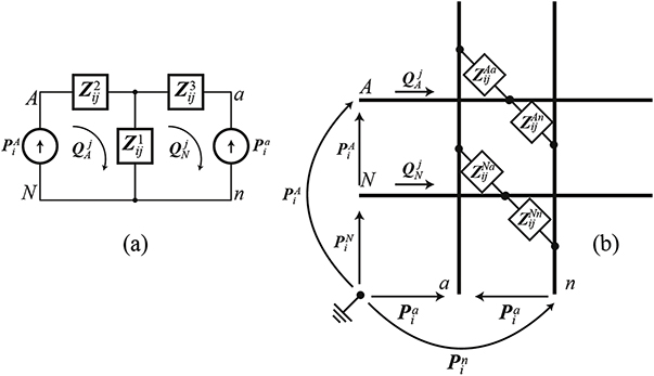
The loop and mesh holor equations method is a convenient means of formulating holor equations when the unknowns are of the energy-transfer-holor type. This method favours the use of impedance-holor parameters.
Let us consider, therefore, the fluidic commutation matrixer shown in figure 13.3. The fluidic commutation
matrixer represents a particular fluidic homogeneous continuous dynamical system that
has input pressure-source holors of sinusoidal type with effective values of
pressure-source holors
 and
and
 .
.
Figure 13.3. Analogous physical commutation matrixer (fluidic commutation matrixer) involving impedance holors.
Download figure:
Standard image High-resolution image
One wants to find holor equations that describe the sinusoidal flow holors through all
the impedance-holor components. In this case, there are three distinct impedance holors
and three distinct flow holors. However, only two of these are independent. For
instance, if
 is the flow holor through
 , and
, and
 is the flow holor through
 , then the flow holor through
 is
is
 .
.
The flow holors
 and
and
 are the mesh flow holors and they are the
most convenient choice for the unknowns, since one may apply equation (10.1b) around the
closed mesh.
are the mesh flow holors and they are the
most convenient choice for the unknowns, since one may apply equation (10.1b) around the
closed mesh.
If one applies equation (10.1b) around meshes A and a:


The meshes are the open spaces in the impedance-holor fluidic commutation matrixer.
One always takes the flow holor in each mesh in a clockwise sense of direction. One may now substitute the fluidic commutation matrixer component relations into the mesh equations (13.6a) and (13.6b) to obtain:


Alternatively, if one groups the flow holors together in equation (13.7) the result is:


One may interpret the terms in equation (13.8) as follows.
- In mesh A:
 —the sum of the pressure-holor drops
across each impedance holor in a sense of the flow-holor direction and due to
—the sum of the pressure-holor drops
across each impedance holor in a sense of the flow-holor direction and due to
 only; all the other flow holors are set
to zero;
only; all the other flow holors are set
to zero; —the sum of the pressure-holor
drops across impedance holors, in a sense of direction
—the sum of the pressure-holor
drops across impedance holors, in a sense of direction
 , but due to flow holor
 ; all the other flow holors are
set to zero;
; all the other flow holors are
set to zero;
- In mesh a:
 —the sum of the pressure-holor drops in
mesh a in a sense of flow direction due to
—the sum of the pressure-holor drops in
mesh a in a sense of flow direction due to
 ; all the other holor flows are set to zero;
 —the sum of the pressure-holor
drops due to holor flow
—the sum of the pressure-holor
drops due to holor flow
 ; all the other flow holors are
set to zero.
; all the other flow holors are
set to zero.
In matrix form, equation (13.8) may be written as:
In the impedance-holor array, the terms on the main diagonal are positive and all others are negative. This is true for mesh holor equations when the assumed senses of flow direction are all clockwise or all counter clockwise.
The general form for the mesh holor equations is:
The fluidic-commutation-matrixer component
 is the sum of all the impedance holors in
mesh A and
is the sum of all the impedance holors in
mesh A and
 is the sum of all the impedance holors in
mesh a. The impedance holors
is the sum of all the impedance holors in
mesh a. The impedance holors
 and
and
 are equal and are the negative of all the
common terms in
are equal and are the negative of all the
common terms in
 and
and
 , provided that all the circulating flow
holors are taken in the same sense of direction (e.g. all clockwise).
, provided that all the circulating flow
holors are taken in the same sense of direction (e.g. all clockwise).