
Resonances and compound reactions
Published October 2015
•
Copyright © IOP Publishing Ltd 2015
Pages 11-1 to 11-11
You need an eReader or compatible software to experience the benefits of the ePub3 file format.
Download complete PDF book or the ePub book

Permissions
Abstract
Although resonances occur in direct, intermediate and compound reactions they are most obvious in the latter case. A long-lived compound system will have narrow resonance structures described by the characteristic Breit–Wigner form. Each resonance corresponds to an excited nuclear state in the continuum, often with a very long lifetime (<10−16 s). Prominent examples are the neutron resonances in heavy nuclei. A compound system has time to 'forget' its formation, and re-emission of a particle ideally occurs out of thermodynamic equilibrium (by evaporation). At higher excitations resonances become wider and more numerous and can only be described with statistical methods (Ericson fluctuations and Hauser–Feshbach theory).
11.1. Generalities
Resonances are a very general phenomenon in nature and therefore in all of physics, see also chapter 6. In classical physics they appear when a system capable of oscillations is excited with one or more of its eigenfrequencies, which—depending on the degree of damping—may lead to large oscillation amplitudes of the system. Nuclei are no exception. When tuning the system (changing the exciting frequency) these amplitudes pass through a resonance curve of Lorentz form. In particle physics most of the many known 'particles' actually appear as resonances, i.e. as quantum states in the continuum, which decay with characteristic widths (or, equivalently, lifetimes).
Resonances can be discussed in the energy picture where, as a function of energy, excursions of Lorentz form (Breit–Wigner form) with a width Γ appear, and also in the complementary time picture where they appear as quantum states in the continuum, i.e. as states which decay with finite lifetime τ. Between them there is the relation

In nuclear physics resonances appear in the continuum (i.e. in scattering situations, at positive total energy) when the projectile energy in the center-of-mass system plus the Q-value of the reaction just equals the excitation energy of a nuclear state.
The excitation functions of observables such as the cross section show characteristic excursions from the smooth background when varying the incident energy. The background may be due to a direct-reaction contribution from Coulomb or shape-elastic scattering or—in a region of high-level density—may be the energy-averaged cross section of unresolved overlapping compound resonances; in this case resonant excursions would be due to doorway mechanisms. Likewise the scattering phases and scattering amplitudes change in characteristic ways over comparatively small energy intervals. Nuclei may be excited into collective modes such as rotations and/or vibrations of a part of the nucleons. At still higher energies new phenomena with high cross sections in charged-particle, neutron, γ and π induced reactions appear involving up to all nucleons of a nucleus, the giant resonances. Figure 11.1 shows the phenomena schematically in different energy regions.

Figure 11.1. The excitation of single resonances, overlapping resonances (with and without Ericson fluctuations) and giant resonances as functions of the energy in the continuum region above the bound-state energy.
Download figure:
Standard image High-resolution image11.2. Theoretical shape of the cross sections
A model assumption for resonances is—in contrast to direct processes—that the system goes via an intermediate state from entrance into the exit channel. For this case perturbation theory gives the following form of the transition matrix element

 is the energy of the nuclear eigenstate. However, since it is a state
in the continuum it is not stationary but one which decays in time. Such states are best
described by giving them a complex eigen-energy:
is the energy of the nuclear eigenstate. However, since it is a state
in the continuum it is not stationary but one which decays in time. Such states are best
described by giving them a complex eigen-energy:

The interpretation of the imaginary part is: the time development of a
state has the form  , on the other hand the state decays with a lifetime
τ, whence
, on the other hand the state decays with a lifetime
τ, whence

The resonance amplitude thus has the form:

The meaning of F(E) has to be determined. In the sense of Bohr's independence hypothesis, the formation and decay of a resonance are independent (i.e. decoupled). Therefore, one writes the amplitude as the product of the probability amplitude for its formation and its probability of decaying into the considered exit channel. In general, for one formation channel (the entrance channel c) there will be several exit channels c'.
The width Γ of the Breit–Wigner function is inversely proportional to the formation probability P and is the integral over the cross section in the energy range of the resonance:
In equilibrium this is equal to the probability that the resonance
re-decays into the entrance channel (the purely elastic case). A measure for this is the
partial width  formed similarly to Γ, thus:


By definition Γ is the sum of all partial widths over the open channels.
Thus, the branching ratio for the decay into one definite channel  is equal to
  and the Breit–Wigner cross section for the formation of the resonance
via channel c and the decay via channel c'
is
and the Breit–Wigner cross section for the formation of the resonance
via channel c and the decay via channel c'
is

This derivation is simplified and must be carried out—when there is interference with a direct background contribution and for the description of a differential cross section via a partial-wave expansion near a resonance—with complex scattering amplitudes. For elastic s-wave scattering this results in a resonant scattering amplitude of the form:

When a direct background is present, in addition to the pure resonance term and the pure direct (smooth) term, a typical interference term appears, which may be constructive or destructive. For σ we have then:

where  is the amplitude of the weakly energy-variable potential
scattering.
is the amplitude of the weakly energy-variable potential
scattering.
11.3. Derivation of the partial-width amplitude for nuclei (s-waves only)
The connection between the resonant scattering wave function and the wave function of the eigenstate of the nucleus is made using the R-matrix theory. Their basic features (for more details see [20]) are approximately:
- •The two wave functions and their first derivatives are matched continuously at the nuclear radius (the edge of the potential or similar).
- •The condition for a resonance is equivalent to the wave-function amplitude in the nuclear interior taking on a maximum value. This happens exactly if the matching at the nuclear radius occurs with a wave function with gradient zero (horizontal tangent).
Figure 11.2 illustrates the conditions for resonance. The two conditions may be summarized such that both logarithmic derivatives L (L0 for pure s-waves) at the nuclear radius are exactly zero. With the form of the wave function in the external region

and the wave numbers in the external k in the nuclear interior κ we obtain

which leads to the scattering function  as a function of L0:

Inserting this scattering function into the known expressions for elastic
scattering and absorption (and with  ) the result is

and

By expanding  in a Taylor series and terminating it after the first term, by
comparison—in addition to obtaining the resonance scattering amplitude (with
in a Taylor series and terminating it after the first term, by
comparison—in addition to obtaining the resonance scattering amplitude (with  )—one obtains the results:


One sees that in agreement with our definition of absorption this encompasses all exit channels except the elastic channel.

Figure 11.2. Boundary conditions at the nuclear (potential) surface for the appearance of a resonance in the excitation function.
Download figure:
Standard image High-resolution image11.4. The first evidence of resonant nuclear reactions
Around 1934/1935 two models of nuclear interaction were put forward and debated:
- •The single-particle model, which describes the interaction of a nucleon with nuclei as a global interaction with each nucleus as a whole with very little regard for the internal structure. Elastic processes should therefore depend only weakly on the mass number of the target nuclei, predominantly via the radius dependence with A, and also on the incident energy, a concept realized in the optical model, see chapter 10. Inelastic processes should be fast, peripheral and involve only very few nucleons.
- •The compound-nucleus model relies on the assumption that an incident nucleon (or other nucleus) is absorbed by the target nucleus, shares its properties such as mass, energy and spin with all nucleons, and may be emitted after a long delay by thermal excitation (evaporation, compound-elastic scattering) or another nucleon or a group of nucleons is evaporated in the same way (compound-nuclear (CN) reaction).
The applicability of each model could only be decided experimentally. E P Wigner gives a good account of these early developments. His statement, cited from [28], 'Experimental work constituted, in my opinion, the most important step in the development', expresses this.
11.5. Neutron resonances
In the years around 1934 Enrico Fermi and his collaborators (Amaldi et
al [1–3, 13]) performed experiments in Rome with
neutrons, especially slow neutrons that were produced by slowing down fast neutrons in
hydrogenous materials. The fast neutrons were produced in ( ) reactions on nuclei such as
  with α particles from radium, radon, or polonium
sources. Figure 11.3 shows
a typical set-up of a neutron source surrounded by a paraffin moderator, a target
absorber and a detector for capturing γ radiation. An energy variation
was achieved by changing the temperature environment with which the neutrons became
equilibrated. Their very systematic studies of capture reactions revealed very different
cross sections for different elements. Very high absorption was observed for B and Cd,
but only for very slow neutrons, also on many other nuclei without any systematics
between neighboring nuclei. Other groups also studied the interaction of neutrons with
nuclei. Other key experiments are those of Bjerge et al [5], Dunning et
al [11],
Szilard [24] and Moon
et al [21, 22]. In
these experiments the 'selective absorption' of slow neutrons by different nuclei was
investigated by studying the emission of γ after absorption of the
neutrons as a function of energy and for different nuclei. One has to keep in mind that
neutron physics was difficult in many respects (e.g. in determining their energies,
making sure that the neutrons were really thermal, their proper collimation, background
shielding and their detection). Nevertheless the results were that absorption cross
sections differed so widely between different nuclei that a simple absorption law
with α particles from radium, radon, or polonium
sources. Figure 11.3 shows
a typical set-up of a neutron source surrounded by a paraffin moderator, a target
absorber and a detector for capturing γ radiation. An energy variation
was achieved by changing the temperature environment with which the neutrons became
equilibrated. Their very systematic studies of capture reactions revealed very different
cross sections for different elements. Very high absorption was observed for B and Cd,
but only for very slow neutrons, also on many other nuclei without any systematics
between neighboring nuclei. Other groups also studied the interaction of neutrons with
nuclei. Other key experiments are those of Bjerge et al [5], Dunning et
al [11],
Szilard [24] and Moon
et al [21, 22]. In
these experiments the 'selective absorption' of slow neutrons by different nuclei was
investigated by studying the emission of γ after absorption of the
neutrons as a function of energy and for different nuclei. One has to keep in mind that
neutron physics was difficult in many respects (e.g. in determining their energies,
making sure that the neutrons were really thermal, their proper collimation, background
shielding and their detection). Nevertheless the results were that absorption cross
sections differed so widely between different nuclei that a simple absorption law  (as evidenced for fast neutrons as they were produced by the Rn–Be
source) could not be valid. Cross sections of
(as evidenced for fast neutrons as they were produced by the Rn–Be
source) could not be valid. Cross sections of  , respectively, were reported for B, Y and Cd, about 1000 × larger than
for fast neutrons. The idea that with slow (thermal or sub-thermal) neutrons an
, respectively, were reported for B, Y and Cd, about 1000 × larger than
for fast neutrons. The idea that with slow (thermal or sub-thermal) neutrons an  nucleus formed in the neutron capture process became prevalent, but no
explanation of the differing cross sections and their energy dependence emerged.
nucleus formed in the neutron capture process became prevalent, but no
explanation of the differing cross sections and their energy dependence emerged.
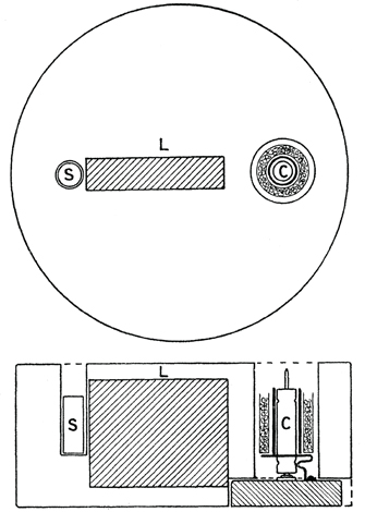
Figure 11.3. Typical set-up for experiments of slow neutron capture. Shown is the Po/Be source S in a paraffin block, a lead absorber shield for primary γ L and the detector C, here a Geiger–Müller counter surrounded by the absorber target material [2].
Download figure:
Standard image High-resolution imageLeo Szilard, after another experiment on an In absorber [24], already concluded that 'it would therefore seem that some elements have fairly sharp regions of strong absorption...'. This description fits the properties of what were soon called resonances in the sense described above, but for neutrons they were still described as 'selective absorption' or 'selective capture'.
Experimental progress, particularly in the creation of high energy resolution neutron beams (see also figure 12.8 in chapter 12), was decisive in many respects:
- •The exact Breit–Wigner form plus interference with direct background could be established.
- •The very rich structure of low-lying CN energy levels could be studied.
- •The statistics of level densities and level widths could be established.
- •Near the onset of overlapping of levels, phenomena such as statistical Ericson fluctuations [12] and finally, at still higher excitations, the smooth CN behavior described by Hauser and Feshbach [16] in the statistical model appeared, which had to be distinguished from smooth direct-interaction amplitudes, see e.g. [26, 27].
An example of the resonance behavior that also has practical importance in the
slowing down of reactor neutrons in  is shown in figure 11.4.
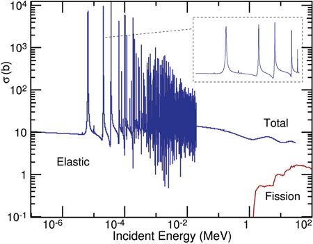
Figure 11.4. Excitation function of the cross section of neutrons interacting with  . At low energies elastic scattering dominates the total cross
section with interference with narrow compound-nucleus resonances. At higher
energies the region of resonances overlaps, then a smooth cross section is visible
and other channels open up, such as fission. Adapted from [23].
. At low energies elastic scattering dominates the total cross
section with interference with narrow compound-nucleus resonances. At higher
energies the region of resonances overlaps, then a smooth cross section is visible
and other channels open up, such as fission. Adapted from [23].
Download figure:
Standard image High-resolution image11.6. Charged-particle resonances
Around the same time as neutron absorption by nuclei, in particular using thermal neutrons, was performed, similar studies, with protons in particular, became feasible with the development of accelerators with higher voltages than the first (Cockroft–Walton) machine. In order to surmount the Coulomb barrier before being absorbed by nuclei the protons had to have energies in the MeV range. Pioneering work was performed at the Department of Terrestrial Magnetism (DTM) of the Carnegie Institution in Washington, DC, by Tuve et al and at Madison by Herb et al. Due to the high energy resolution and stability of the beams from these new accelerators, they were able to measure excitation functions that showed the resonances nicely [14, 15, 25]. As an example, the 2 m open-air Van de Graaff accelerator at DTM that reached 1.3 MeV proton energy is shown in figure 11.5, together with an excitation function of proton scattering from carbon as function of energy. In 1935 R Herb [17] developed the first Van de Graaff accelerator in a pressurized vessel thus providing much higher breakthrough voltages from the accelerator terminal to ground and thus higher maximum voltages, here 2 MV [18], as shown in figure 11.6. This design was the prototype for the many later Van de Graaff accelerators. A large number of nuclei was investigated with protons via the capture reaction. The de-excitation γ rays were registered with an electroscope as shown in figure 11.7. Figure 11.8 shows excitation functions of protons on Li and F targets that clearly exhibit resonance structures, which could be identified with CN states in the corresponding nuclei. Their observation required a sufficiently good energy resolution for the accelerator as well as sufficiently thin targets [19].
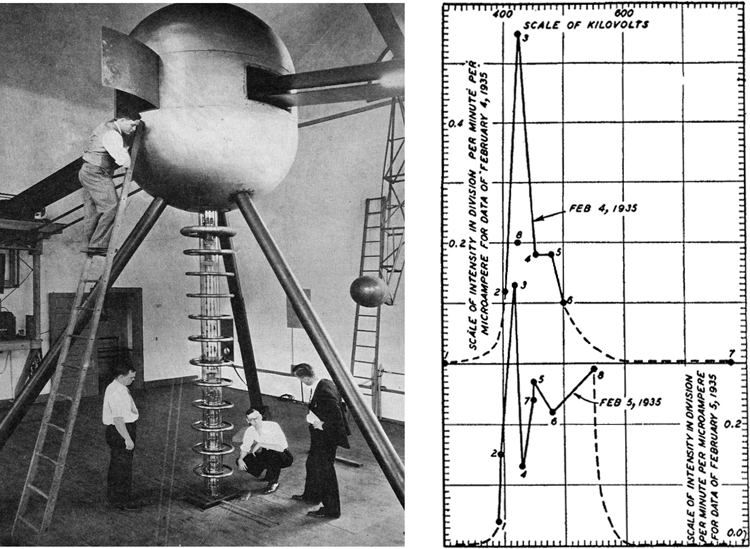
Figure 11.5. The open-air Van de Graaff accelerator at DTM (with paper charging belt) and an excitation function of protons on C showing early evidence of CN resonances in the compound system [14, 25]. Copyright 1935 American Physical Society.
Download figure:
Standard image High-resolution image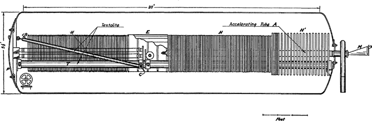
Figure 11.6. The 1937 Madison Van de Graaff accelerator enclosed in a pressure tank. Reproduced with permission from [18]. Copyright 1937 American Physical Society.
Download figure:
Standard image High-resolution image
Figure 11.7. The Madison reaction chamber for (p,γ) capture experiments. Reproduced with permission from [19]. Copyright 1937 American Physical Society.
Download figure:
Standard image High-resolution image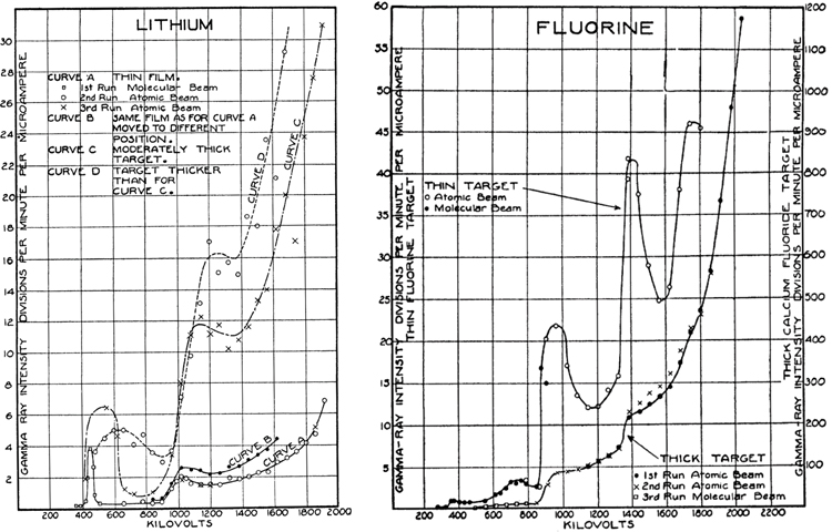
Figure 11.8. Excitation functions of protons scattered from Li and F showing CN resonances. Adapted with permission from [19]. Copyright 1937 American Physical Society.
Download figure:
Standard image High-resolution image11.7. The compound-nucleus model
Niels Bohr [6–9] used the observations of
'selective effects, selective capture, selective absorption' of low-energy neutrons on
the one hand and 'charged-particle resonances' on the other to formulate his model of
the formation of a compound nucleus explaining the properties of the
high cross sections as resonances in the system of the target nuclei plus one neutron
being captured to form a highly excited, rather long-lived nuclear state (lifetimes up
to  times longer than the traversal time). Among the properties of the
compound nuclei was their decay independent of their formation
(Bohr's independence hypothesis). Bohr presented the
famous drawing explaining the CN interaction between a nucleon and a target nucleus
[7], depicted in figure
11.9. Bohr [6–9], Breit and Wigner [10], and Bethe [4] were the main early proponents of the
compound-nucleus model of nuclear reactions.
times longer than the traversal time). Among the properties of the
compound nuclei was their decay independent of their formation
(Bohr's independence hypothesis). Bohr presented the
famous drawing explaining the CN interaction between a nucleon and a target nucleus
[7], depicted in figure
11.9. Bohr [6–9], Breit and Wigner [10], and Bethe [4] were the main early proponents of the
compound-nucleus model of nuclear reactions.

Figure 11.9. Bohr's illustration of the compound-nucleus process. Reproduced with permission from [7]. Copyright 1936 Nature Publishing Group.
Download figure:
Standard image High-resolution image
References
- [1]Amaldi E and Fermi E 1936 Ric. Sci. A 6 544
- [2]Amaldi E, D'Agostino O, Fermi E, Pontecorvo B, Rasetti F and Segrè E 1935 Proc. R. Soc. A 149 522
- [3]Amaldi E and Fermi E 1936 Ric. Sci. 1 310
- [4]Bethe H A 1937 Rev. Mod. Phys. 9 69
- [5]Bjerge T and Westcott C H 1935 Proc. R. Soc. A 150 709
- [6]Bohr N 1936 Nature 137 344
- [7]Bohr N 1936 Nature 137 351
- [8]Bohr N and Kalckar F 1937 Mat.-Fys. Medd. K. Dan. Vidensk. Selsk. 27 no. 10
- [9]Bohr N 1937 Science 86 161
- [10]Breit G and Wigner E 1937 Phys. Rev. 49 519
- [11]Dunnning J R, Pegram G B, Fink G A and Mitchell D P 1935 Phys. Rev. 48 265
- [12]Ericson T and Mayer-Kuckuk T 1966 Ann. Rev. Nucl. Sci. 16 183
- [13]Fermi E, Amaldi E, D'Agostino O, Rasetti F and Segrè E 1934 Proc. R. Soc. A 146 483
- [14]Hafstad L R and Tuve M A 1935 Phys. Rev. 48 306
- [15]Hafstad L R, Heydenburg N P and Tuve M A 1936 Phys. Rev. 50 504
- [16]Hauser W and Feshbach H 1952 Phys. Rev. 87 366
- [17]Herb R G, Parkinson D B and Kerst D W 1935 Rev. Sci. Instrum. 6 261
- [18]Herb R G, Parkinson D B and Kerst D W 1937 Phys. Rev. 51 75
- [19]Herb R G, Parkinson D B and Kerst D W 1937 Phys. Rev. 51 691
- [20]Lane A M and Thomas R G 1958 Rev. Mod. Phys. 30 145
- [21]Moon P B and Tillman J R 1935 Nature 135 904
- [22]Moon P B and Tillman J R 1936 Proc. R. Soc. A 153 476
- [23]National Nuclear Data Center 2012 Brookhaven National Laboratory
- [24]Szilard L 1935 Nature 136 950
- [25]Tuve M A, Hafstad L R and Dahl O 1935 Phys. Rev. 48 315
- [26]Vogt E 1968 (New York: Plenum) The Statistical Theory of Nuclear Reactions (Advances in Nuclear Physics vol 1) p 261
- [27]Vogt E 1972 Rev. Mod. Phys. 34 723
- [28]Wigner E 1955 Am. J. Phys. 23 371