Theory of optical propagation and diffraction
Published August 2014
•
Copyright © IOP Publishing Ltd 2014
Pages 1-1 to 1-6
You need an eReader or compatible software to experience the benefits of the ePub3 file format.
Download complete PDF book or the ePub book

Permissions
Abstract
Beginning with Maxwell's equations, the wave equation is derived. This is followed by derivations of the integral theorem of Helmholtz and Kirchoff, and the Rayleigh-Sommerfeld diffraction formulae.
1.1. The Helmholtz equations
1.1.1. The wave equation in the time domain
We start with Maxwell's equations which describe the interaction between an electric field vector E (Ex , Ey , Ez ) and a magnetic field vector H (Hx , Hy , Hz ).
This assumes that there is no free charge; μ is the permeability and ε the permittivity of the propagation medium. Both electric and magnetic field vectors are functions of both position and time, represented by their Cartesian components and the time derivative.
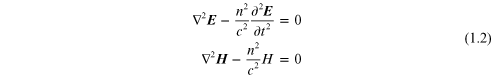
The equations can be combined by taking the cross-product of the first two time-derivative equations, which results in the wave equations.
We assume that the medium is linear, isotropic, non-dispersive and
homogeneous. That is, ε and μ are
constant. We define ε0 and μ0 as the constants in a vacuum. The refractive index is  and the velocity of propagation in a vacuum is
  . The vector equations are obeyed by both the electric
and magnetic fields and there is a scalar equation that is obeyed by
each component of the fields. The expression for the
x-component of the electric field equation
becomes
. The vector equations are obeyed by both the electric
and magnetic fields and there is a scalar equation that is obeyed by
each component of the fields. The expression for the
x-component of the electric field equation
becomes

Now we can generalize to any scalar field component u(x, y, x, t)

Reducing the vector equations to scalar equations has consequences. If a medium is inhomogeneous where ε depends on position, a coupling occurs between the components of the fields and all components will not necessarily satisfy the same wave equation. Furthermore, at an interface between two media, the boundary conditions must be satisfied over a small region where an error occurs between the vector results and the scalar approximation. This is the crux of the study of Fourier optics. By making more simplifying assumptions about the propagation conditions, which result in simpler and more solvable equations, errors in the details appear. By limiting the errors, we can use simpler expressions and many useful mathematical tools to provide practical results.
Instead of using the Cartesian coordinates x,
y, z, we can combine the spatial
coordinates into one three-dimensional coordinate, s.
Let us assume that we have a monochromatic wave that must satisfy the
wave equation. The wave number k is given by  where λ is the wavelength. And, where
the velocity in the homogeneous dielectric medium is ν,
the wavelength is defined as
where λ is the wavelength. And, where
the velocity in the homogeneous dielectric medium is ν,
the wavelength is defined as  . One solution that represents a traveling wave
is
. One solution that represents a traveling wave
is

A(s) is the wave amplitude and ϕ(s) is the wavefront phase. Knowing that the Laplacian is

Equation (1.5) satisfies the time independent wave equation

There are many solutions to the wave equation. Waves can be traveling spherically from a source point. They can be plane waves where the plane is normal to the direction of propagation. Depending upon the boundary conditions and source of the radiation, they can take on many different forms. In 1678 Christian Huygens stated that any wavefront of a field that satisfies the wave equation can be considered to be made up of an infinite number of spherical source points that form a new wavefront as it propagates. See figure 1.1.
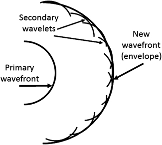
Figure 1.1. Huygens' spherical wavelets form a new wavefront.
Download figure:
Standard image High-resolution image
1.2. The integral theorem of Helmholtz and Kirchhoff
We quantify this by solving the spherical wave problem using Green's theorem. Most calculus texts cover the proof and general application of the theorem, but because I absolutely abhor rigorous mathematical proofs, I will avoid repeating it here. It is stated simply as an equality between the energy leaving a volume being equal to the energy leaving a surface enclosing the volume in a direction normal to that surface:

The partial derivatives are in the direction of an outward normal to the surface. The point of observation is P0. The surface S surrounds the point P0. Kirchhoff chose the so-called free space Green's function to be a spherical wave expanding about the point P0.
The Green's function at any point P1 at a distance r01 from P0 is

and

The cosine term is the cosine of the angle between the outgoing normal vector
n
and the vector  .
.
After a page or so of mathematics found elsewhere (Goodman 2005) the result is an integral expression for the field at P0 as a function of the field at P1. The result, known as the integral theorem of Helmholtz and Kirchhoff (Kirchhoff 1883) is

The choice of the surface or surfaces of integration is critical to the validity of the result. In many cases involving practical diffraction problems, one of the surfaces will be a sphere of some radius R'. For the integrals to be performed, we want to guarantee that we are dealing with only an outgoing wave through the surface. We have to ensure that the field U vanishes at least as fast as the diverging spherical wave. To do so, we invoke the Sommerfeld radiation condition

1.2.1. The Kirchhoff boundary conditions
Let us now assume that we have a propagating electromagnetic field
impinging on an opaque screen where diffraction occurs due to some
opening in the screen. We want to calculate the field at points behind
the screen. To use the formulation so far described, we have to assert
two conditions called the Kirchhoff boundary conditions. The first is
that the surface of integration after the screen is entirely arbitrary
and the field U and its derivative  are exactly the same as they would be in the absence
of the screen. The second condition is that the screen is really opaque,
that is, in the geometrical shadow of the screen, the field
U and its derivative
are exactly the same as they would be in the absence
of the screen. The second condition is that the screen is really opaque,
that is, in the geometrical shadow of the screen, the field
U and its derivative  are identically zero. These conditions are generally
met if the opening in the screen (the aperture) is large compared to the
wavelength.
are identically zero. These conditions are generally
met if the opening in the screen (the aperture) is large compared to the
wavelength.
1.2.2. The Fresnel–Kirchhoff diffraction formula
Another simplification can be made, if the distance r01 is large compared to the wavelength, the  term in equation (jk). If the
aperture is illuminated by a single spherical wave at point
P2,
term in equation (jk). If the
aperture is illuminated by a single spherical wave at point
P2,

the field at P0 reduces to the Fresnel–Kirchhoff diffraction formula:

The integration is now over the aperture in the region around P1. This equation is symmetrical between P0 and P2. The field at P0 from the source at P2 through the aperture would be the same as the field at P2 from a point source at P0. The fact that light and diffraction do not seem to care whether the beam is going left-to-right or right-to-left is known as the reciprocity theorem of Helmholtz:

where

The r vectors end in the aperture at P1. As one moves across the aperture, the directions of the r vectors change and it appears that the field in the aperture is an infinite number of secondary spherical waves that match the Huygens principle. Fresnel made the Huygens assumption work along with Young's principle of interference and Kirchhoff showed that this property was a fundamental part of the nature of light itself.
1.3. The Rayleigh–Sommerfeld formulation of diffraction
Not all apertures are illuminated by a point source of light in front of the aperture. To expand to practical light sources with varying amplitudes and phases, the Rayleigh–Sommerfeld formulation is produced. Kirchhoff theory imposed two conditions on both the field amplitude and its derivative.
Going back to the Green's function solution for the field at P0,

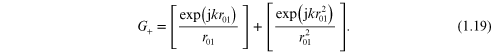
where ![$G=[\frac{{\rm exp} ({\rm j}k{{r}_{01}})}{{{r}_{01}}}]$](https://content.cld.iop.org/books/10__1088_978-0-750-31056-7/revision2/bk978-0-750-31056-7ch1ieqn29.gif) .
.
Sommerfeld found a Green's function that allowed either G or  to vanish without requiring both to vanish on the
aperture. He introduced another source point
to vanish without requiring both to vanish on the
aperture. He introduced another source point  at a mirror image of the observation point P0.
The first Rayleigh–Sommerfeld solution is
at a mirror image of the observation point P0.
The first Rayleigh–Sommerfeld solution is
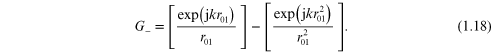
The new source at  is 180˚ out of phase with the point P0 so the
field vanishes on the screen and aperture.
is 180˚ out of phase with the point P0 so the
field vanishes on the screen and aperture.
The second Rayleigh–Sommerfeld solution is
The new source at  is in phase with the point P0 so the normal
derivative of the field vanishes on the screen and aperture. After about two
pages of mathematical rigor, we find two results for the field at
P0 due to a spherical wave source at
P2.
is in phase with the point P0 so the normal
derivative of the field vanishes on the screen and aperture. After about two
pages of mathematical rigor, we find two results for the field at
P0 due to a spherical wave source at
P2.


The Fresnel–Kirchhoff formulation, (1.14), and the two
Rayleigh–Sommerfeld integrals, (1.20) and (1.21),
all describe the radiation field at point P0 as a sum of
diverging spherical waves across the aperture much like Huygens' model. For
cases many wavelengths from the aperture, the Fresnel–Kirchhoff solution has
been shown to be the average of the two Rayleigh–Sommerfeld solutions. Only
where the cosine terms (the obliquity factors) are significant near the
aperture do these theories differ. The Huygens–Fresnel principle can be
simplified by describing the combination of spherical waves in the aperture
as a single field  .
.
References
- Goodman J W 2005 Introduction to Fourier Optics 3rd edn (Englewood, CO: Roberts)
- Kirchhoff G 1883 To the theory of light beams Ann. Phys. Lpz. 254 663–95