
Abstract
An X-ray tomographic technique was developed to investigate the internal magnetic domain structure in a micrometer-sized ferromagnetic sample. The technique is based on a scanning hard X-ray nanoprobe using X-ray magnetic circular dichroism (XMCD). From transmission XMCD images at the Gd L3 edge as a function of the sample rotation angle, the three-dimensional (3D) distribution of a single component of the magnetic vector in a GdFeCo microdisc was reconstructed with a spatial resolution of 360 nm, using a modified algebraic reconstruction algorithm. The method is applicable to practical magnetic materials and can be extended to 3D visualization of the magnetic domain formation process under external magnetic fields.
Export citation and abstract BibTeX RIS

Content from this work may be used under the terms of the Creative Commons Attribution 4.0 license. Any further distribution of this work must maintain attribution to the author(s) and the title of the work, journal citation and DOI.
Magnetic domain structures1) are known to reflect the fundamental magnetic properties of materials, such as magnetostatic interaction, exchange energy, and magnetic anisotropy. Nucleation of magnetic domains and pinning of domain-wall propagation govern the magnetization-reversal processes and determine the macroscopic coercivity. Therefore, observation of the magnetic domain structure is important for understanding the magnetic characteristics of systems, including practical magnetic materials. Since the first confirmation of domain structure by Bitter,2) researchers have developed a variety of domain observation techniques, including magneto-optical Kerr effect (MOKE) microscopy,1) magnetic force microscopy,3) Lorentz transmission electron microscopy,4) scanning probe magnetic microscopy,5) photoelectron emission microscopy (PEEM),6) and transmission soft X-ray microscopy in the scanning and full-field imaging schemes.7,8) These techniques have been utilized in scientific and industrial fields. However, most of them are limited to the observation of surfaces where the magnetic domain structures are two-dimensional (2D). Transmission microscopy is used to obtain magnetic domain images of thin films with thicknesses of less than ∼100 nm, in which signals are averaged over the thickness direction even though the film could have a three-dimensional (3D) nano-spin texture. Investigating the internal domain structure of ferromagnets is of great technological importance for improving the performance of bulk permanent magnets, which are used in motors for electric cars and electricity generators for wind-power plants. To this end, a new microscopy technique is needed to directly observe the interior magnetic domain structures of bulk ferromagnets. It should be a magnetic counterpart of computed tomographic observation, which allows the 3D visualization of magnetization distributions on the nanoscale.9)
A few studies involving successful 3D domain observations have been reported thus far. A tomographic technique involving neutron Talbot interferometry was used to visualize magnetic domains within a bulk FeSi crystal at a resolution of 35 µm.10) Electron holographic vector field electron tomography was utilized to reveal the magnetic field vector structures of magnetic vortices.11) By using the synchrotron X-ray technique, Streubel et al. observed the pseudo 3D magnetic domain of a tubular magnetic film via the combination of soft X-ray microscopy and PEEM.12) Donnelly et al. recently reported the 3D observation of vector domains of GdCo2 alloys via X-ray ptychography.13) However, there have been few studies, and it is important to develop different approaches of 3D magnetic microscopy for extending the capabilities and applicability of this emerging technique.
In this study, we demonstrate magnetic tomography via scanning hard X-ray microscopy based on X-ray magnetic circular dichroism (XMCD).14) We present the feasibility of the technique for studying a microfabricated structure of the soft ferromagnet GdFeCo, overcoming the limitations of neutron, electron, and soft-X-ray probes.10–12) The technique adopts a flexible setup enabling future studies under external fields and in combination with X-ray fluorescence microtomography,15) which is a potential advantage over hard X-ray ptychographic techniques.13)
A magnetic film of SiN (60 nm)/Gd22.00Fe68.25Co9.75 (5,000 nm)/SiN (5 nm) was grown on a SiN membrane substrate with a thickness of 1 µm via magnetron sputtering and was then fabricated into a disc shape via optical lithography and Ar ion milling. The designed diameter and the thickness were 10 and 5 µm, respectively. Our MOKE measurement revealed the perpendicular magnetization of the unpatterned film. Maze-like domain structures with stripe widths of 2–3 µm were observed at the remanent magnetization state. From an XMCD measurement at the Gd L3 edge, the XMCD contrast of ±5% with respect to the polarization-averaged X-ray absorption coefficient was obtained. Element-specific magnetization measurement in the unpatterned film revealed a characteristic hysteresis loop with perpendicular magnetization and the formation of multiple domain structures. The coercivity of the unpatterned film was estimated to be ∼50 Oe.
Magnetic X-ray computed tomographic imaging measurement was performed using the scanning hard X-ray nanoprobe at BL39XU of the SPring-8 synchrotron radiation facility.16) Figure 1 shows the experimental setup. The X-ray energy was tuned at the L3 resonance of Gd (7.247 keV), at which the maximum XMCD contrast was obtained, using a Si 111 double-crystal monochromator. A 0.45-mm-thick diamond X-ray phase retarder was used to generate circularly polarized X-ray beams of switchable photon helicity. The degree of circular polarization was greater than 99% for both helicities. A Kirkpatrick–Baez mirror was used to focus the circularly polarized X-ray beam. The spot size was estimated to be 130 (horizontal) × 140 (vertical) nm2 in full width at half maximum (FWHM) via the knife-edge scan method. The distance between the mirror end and the sample was 100 mm. The depth of focus was 100 µm, which was much greater than the sample diameter and the eccentric radius of the sample rotation stage.
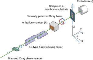
Fig. 1. Experimental setup of the magnetic tomography measurement based on the scanning hard X-ray nanoprobe.
Download figure:
Standard image High-resolution imageThe GdFeCo microdisc on the SiN membrane substrate was placed at the focal point of the X-ray beam, mounted on a stepping motor-driven X–Z translation stage and a rotation stage along the vertical (Z) axis. The X translation stage was equipped with the optical encoder and closed-loop feedback. The Z translation stage was in open-loop control with a resolution of 50 nm. The rotation stage was equipped with an air-bearing mechanism of extremely low wobble, ensuring an eccentric radius of <1 µm for a full 360° of rotation.
Projected magnetic images were collected via scanning XMCD microscopy as a function of the angle of sample rotation. A 2D XMCD image was recorded via raster scanning of the sample position in the plane perpendicular to the direction of the incoming X-ray beam. The sample position in the horizontal (X) direction was scanned continuously for acquisition of the one-pixel line, at a velocity of 1 µm/s, while the vertical (Z) position of the sample was moved by a 100-nm step. The intensity of the X-ray beam incident on the sample (I0) was monitored using an ionization chamber. The transmitted X-ray intensity (I) was measured using a silicon PIN photodiode detector. The XMCD magnetic contrast is defined as Δμ = μ+ − μ−, where  [
[ ] is the absorption coefficient determined from the incident
  (
( ) and transmitted I+ (I−) X-ray intensities, for right (left) circular polarizations, respectively. The polarization-averaged X-ray absorption spectroscopy (XAS) signal, which corresponds to the density contrast of the sample, is defined by
  . The photon helicity was switched at 37 Hz, and the lock-in detection technique17) was used to improve the signal-to-noise ratio of the dichroic signal. The time constant of the low-pass filter was 30 ms. The output of voltages of the lock-in amplifier were converted into transistor–transistor logic pulses at the corresponding frequency using a voltage–frequency converter and then counted at a 100-ms duration synchronously with the position encoder output pulses of the X stage. These data-acquisition conditions ensured that the spatial resolution for the X-direction was approximately 100 nm, assuming the scan velocity, sampling rate, and time constant of the lock-in amplifier. The mechanical spatial resolution for the Z-direction was 100 nm, as determined by the scan step of the translation stage. The mechanical resolutions in the X- and Z-directions were smaller than the focused X-ray beam size (130 × 140 nm2 in FWHM), and the practical resolution was determined by the focused X-ray beam size. The projected images of XMCD,
  and XAS
  were collected at angles of −70 to +70° with a step of 5°. The blind regions (−90° < θ < −70°, 70° < θ < 90°) were due to the window size of the membrane substrate. The XAS and XMCD projections were acquired simultaneously, and the acquisition time was 30 min for each projection angle.
We show that conventional reconstruction algorithms can be applied for reconstructing the 3D magnetic domain structure in the case where the sample has strong uniaxial anisotropy and a domain structure with uniaxial magnetization is formed. The bottom of Fig. 2 shows a one-pixel slice of the distribution of the sample magnetization in the X–Y plane, which is perpendicular to the Z-axis for rotation. The X–Y coordinate system is fixed to the X-ray beam and the experimental system, whereas the x–y coordinate system is assumed to be fixed at the sample and rotates about the Z-axis by an angle of θ. In this geometry, the XMCD amplitudes Δμi from a local part of the sample are proportional to the magnetization of the local volume —  — projected to the direction of the incident X-ray beam; i.e.,
  . As shown in the top of Fig. 2, the XMCD projection is given by an integral of Δμi along the X-ray path, which is parallel to the Y-direction:
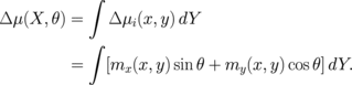
We assume that the sample has strong magnetic uniaxial anisotropy so that only the magnetization component is parallel to the y-direction and the other components are zero; i.e.,  . In this case, XMCD projection is given by

This formula is similar to the Radon transform18) but includes an additional factor of cos θ. If a proper correction for this factor is made, a conventional reconstruction algorithm can be directly applied for reconstruction of the 3D magnetic domains. We preprocessed the recorded projected XMCD images, as follows:

By dividing the original projection image by a factor of cos θ, one may obtain a corrected projection of  , which can be regarded as the Radon transform of the distribution of the uniaxial magnetization,
  . The standard algebraic reconstruction technique19) was applied to 29 projected images taken in the angular range of −70 to 70° with ∼50 iterations. No extrapolation or complement procedure was applied for lacking angles of −90° < θ < −70° and 70° < θ < 90°.
Fig. 2. Principle of the tomographic reconstruction of the magnetization distribution from the projected image of XMCD.
Download figure:
Standard image High-resolution imageFigure 3 shows selected images of the (a) XAS projection and the (b) corresponding XMCD projection of the GdFeCo disc recorded at different angles. The origin of θ was defined as the angle at which the normal of the sample substrate was parallel to the X-ray beam direction. As shown in the XAS image taken at θ = 0°, the sample shape differs from the designed circular shape. The observed diameter of approximately 7 µm was smaller than the designed value of 10 µm, probably because of over-etching in the Ar ion-milling process. Nevertheless, the outline shapes of the disc agreed well between the XAS and XMCD projected images. The XMCD images demonstrate the clear magnetic contrasts of magnetic domains with the typical width of ∼1 µm. The magnetic contrast is the highest in the image taken at 0° and decreases at lager angles. This result provides evidence in support of the perpendicular magnetic domains.

Fig. 3. Selected images of the 2D projections of a GdFeCo disc at different rotation angles obtained using (a) polarization-averaged X-ray absorption and (b) XMCD signals.
Download figure:
Standard image High-resolution imageFigure 4(a) shows a birds-eye view of the 3D reconstruction of the XAS, which corresponds to distributions of the X-ray linear absorption coefficient or the mass density. The images in Fig. 4 were generated using the software ImageJ with the 3D Viewer plugin.20,21) The reconstructed results shown in Figs. 4(a)–4(g) have been trimmed for clarity. In the original reconstructed results, artifacts remain, mostly in the outside regions of the disc, owing to the limited angular range of the projections (see the online supplementary data at http://stacks.iop.org/APEX/11/036601/mmedia). To eliminate the artifacts, voxels having X-ray absorption coefficient values smaller than 25% of the maximum value are masked in the presented images to demonstrate the internal distributions of X-ray absorption and magnetization in the sample.

Fig. 4. Tomographic reconstructions of (a) the X-ray absorption coefficient and (b) the magnetization of the GdFeCo disc. (c)–(f) Slices of the 3D magnetization distribution,  , in the x–Z plane perpendicular to the magnetization easy axis, y. (g) Slice in the y–Z plane at the center of the disc [section along the vertical line in (f)] with vertical lines at which the x–Z slices (c)–(f) are made. (h) Slice in the x–y plane at the center of the disc [section along the horizontal line in (f)]. (i), (j) Cross-sectional profile of the magnetization slice (e) along the dotted lines in the x (A–A') and Z (B–B') directions, respectively.
Download figure:
Standard image High-resolution image
The XAS reconstruction revealed the trapezoidal shape of the GdFeCo disc, which had diameter of 6.7 µm and a thickness of 2.5 µm. The sample was mostly homogeneous in composition. In Fig. 4(b), a cutaway view of the XMCD reconstruction result demonstrates the 3D distribution of the magnetization inside the GdFeCo disc. The color scales correspond to the direction and the amplitude of magnetization perpendicular to the film. Five striped magnetic domains were observed: three positive and two negative.
The sliced images of the x–Z plane at different y positions, which are shown in Figs. 4(c)–4(f), reveal that the magnetic domain structures and the boundaries are similar in the planes perpendicular to the film (easy magnetization direction). The cross sections in the y–Z [Fig. 4(g)] and x–y planes [Fig. 4(h)] clearly indicate the straight domain boundaries along the easy axis. This is a direct observation that the perpendicular magnetic domains are formed through the entire volume of the disc. In Figs. 4(i) and 4(j), the spatial resolutions of the 3D XMCD reconstructed image are estimated from the 10–90% widths of the observed domain boundaries under the assumption that the real boundary widths are significantly smaller than the experimental resolution. The resolution in the x- and Z-directions are given by wx = 311 nm and wZ = 360 nm for the same domain boundary. The obtained spatial resolutions are almost three times larger than the X-ray beam size. For the x-direction, this is because of the limited number of projection angles, which may be insufficient for obtaining reconstruction results with the optimum spatial resolutions. Thermal drifts in the sample position during the measurement might degrade the spatial resolutions in both the x- and Z-directions, although positional corrections to the reconstruction algorithm have been made.
As described above, we successfully visualized the magnetization directions and amplitudes of internal magnetic domain structures with a spatial resolution of a few hundred nanometers for a bulk sample a few micrometers thick, which has not yet been simultaneously achieved using the neutron, electron, or soft X-ray probes.10–12) However, the spatial resolution is approximately three times worse than that of magnetic vectortomography using the hard X-ray ptychographic technique.13) Adopting multilayer mirror optics enables focused X-ray beams on the order of sub-10 nm,25) and the spatial resolutions in our scanning setup can be further improved.
The maximum size of observable samples is approximately 10 µm in diameter, which is restricted by strong X-ray absorption for a thick sample. If one adopts the criterion that the transmittance of the sample should be I/I0 > e−2, the measurable sample sizes is estimated to be 14 µm for Nd2Fe14B at the Nd L2 edge (6.24 keV) and 7 µm for Co50Pt50 at the Pt L3 edge (11.6 keV). Preparation of samples having such micrometer sizes is feasible using the focused ion beam technology currently available.
Our technique is applicable to the 3D observation of internal magnetic domain structures in several kinds of soft and hard magnetic materials. In particular, study of the Nd2Fe14B sintered permanent magnet would provide us with insight regarding the origin of the highly coercive field, as the nucleation and evolution of the magnetic domain structure22) should govern the magnetization-reversal mechanism of this material.23,24) The evolution of 3D magnetic domain structures has been intensively studied via numerical simulations24) but has not been elucidated experimentally thus far. To this end, tomographic magnetic imaging measurements involving external magnetic fields that rotate with the sample to keep the domain structure unaffected must be performed. Our scanning hard X-ray tomography setup with the long mirror-sample distance is suitable for introducing a specially designed magnet and allows 3D observation of the nucleation and evolution of magnetic domains under a variable magnetic field. Moreover, the microstructure of the sintered magnet is comprised of a Nd2Fe14B main phase and other several phases with different chemical compositions.23,24) Nd-rich phases surrounding the main phase likely contribute to the nucleation sites, as well as the magnetization-reversal process.22) Our scanning X-ray setup can easily be modified for X-ray fluorescence microtomography15) and used to study the correlation between the magnetic domains and the elemental distribution of the sintered magnet via 3D imaging.
To summarize, we developed a tomographic imaging technique to investigate the internal magnetic domain structure of micrometer-sized ferromagnetic samples based on scanning hard XMCD microscopy. The technique was applied to a GdFeCo disc that exhibited perpendicular magnetic anisotropy, and the interior uniaxial magnetic domain structures were successfully revealed three-dimensionally with a spatial resolution of 360 nm. This hard X-ray magnetic tomography method is applicable to various soft and hard magnetic materials, including strong permanent magnets, which is of great importance for practical applications.
Acknowledgments
The authors thank Oki Sekizawa for the useful comments. The experiments were performed at the SPring-8 synchrotron radiation facility with the approval of JASRI (Proposal Nos. 2016A0905, 2016B0905, and 2017A0905). This work was partly supported by JSPS KAKENHI Grant Numbers 15H05702 and 17H02823. K.-J.K. was supported by a National Research Foundation of Korea (NRF) grant funded by the Korea Government (MSIP) (No. 2017R1C1B2009686).