


Abstract
The 15 yr pulsar timing data set collected by the North American Nanohertz Observatory for Gravitational Waves (NANOGrav) shows positive evidence for the presence of a low-frequency gravitational-wave (GW) background. In this paper, we investigate potential cosmological interpretations of this signal, specifically cosmic inflation, scalar-induced GWs, first-order phase transitions, cosmic strings, and domain walls. We find that, with the exception of stable cosmic strings of field theory origin, all these models can reproduce the observed signal. When compared to the standard interpretation in terms of inspiraling supermassive black hole binaries (SMBHBs), many cosmological models seem to provide a better fit resulting in Bayes factors in the range from 10 to 100. However, these results strongly depend on modeling assumptions about the cosmic SMBHB population and, at this stage, should not be regarded as evidence for new physics. Furthermore, we identify excluded parameter regions where the predicted GW signal from cosmological sources significantly exceeds the NANOGrav signal. These parameter constraints are independent of the origin of the NANOGrav signal and illustrate how pulsar timing data provide a new way to constrain the parameter space of these models. Finally, we search for deterministic signals produced by models of ultralight dark matter (ULDM) and dark matter substructures in the Milky Way. We find no evidence for either of these signals and thus report updated constraints on these models. In the case of ULDM, these constraints outperform torsion balance and atomic clock constraints for ULDM coupled to electrons, muons, or gluons.
Export citation and abstract BibTeX RIS

Original content from this work may be used under the terms of the Creative Commons Attribution 4.0 licence. Any further distribution of this work must maintain attribution to the author(s) and the title of the work, journal citation and DOI.
1. Introduction
The standard model (SM) of particle physics currently provides our best description of the laws governing the universe at subatomic scales. However, it fails to explain several observed properties of our universe, such as the origin of the matter–antimatter asymmetry, the nature of dark matter (DM) and dark energy, and the origin of neutrino masses. These shortcomings have motivated the development of several theories for physics beyond the SM, or BSM theories for short, accompanied by a rich experimental program trying to test them. The generation of gravitational waves (GWs) is a ubiquitous feature of many BSM theories (Maggiore 2000; Caprini & Figueroa 2018; Christensen 2019). These GWs form a stochastic background and propagate essentially unimpeded over cosmic distances to be detected today, whereas electromagnetic radiation does not start free streaming until after recombination. Thus, detecting a stochastic GW background (GWB) of cosmological origin would offer a unique and direct glimpse into the very early universe and herald a new era for using GWs to study fundamental physics.
Cosmological GWBs can be produced by a number of particle physics models of the early universe. Notably, cosmic inflation generically produces GWs (Guzzetti et al. 2016), which may be observable at nanohertz frequencies if their energy density spectrum is sufficiently blue-tilted. Similarly, an enhanced spectrum of short-wavelength scalar perturbations produced during inflation can source so-called scalar-induced GWs (SIGWs; Domènech 2021; Yuan & Huang 2021a). Another potential source of GWs are cosmological first-order phase transitions (Caprini et al. 2016, 2020; Hindmarsh et al. 2021), which proceed through bubble nucleation; bubble collisions and bubble interactions with the primordial plasma giving rise to sound waves contribute to GW production. Finally, topological defects left behind by cosmological phase transitions, such as cosmic strings and domain walls (Vilenkin 1985; Hindmarsh & Kibble 1995; Saikawa 2017), can radiate GWs and hence contribute to the GWB.
The North American Nanohertz Observatory for Gravitational Waves (NANOGrav; McLaughlin 2013) has recently found the first convincing evidence for a stochastic GWB signal, as detailed in Agazie et al. (2023b, hereafter NG15gwb). Analyzing 15 yr of pulsar timing observations, NANOGrav has detected a red-noise process whose spectral properties are common among all pulsars and that is spatially correlated among pulsar pairs in a manner consistent with an isotropic GWB. In the following, we will refer to this observation as "the NANOGrav signal," "the GWB signal," or simply "the signal," keeping in mind the level of statistical significance at which the GW nature of the signal has been demonstrated in NG15gwb. While the GWB is primarily expected to arise from a population of inspiraling supermassive black hole binaries (SMBHBs; Rajagopal & Romani 1995; Jaffe & Backer 2003; Wyithe & Loeb 2003; Sesana et al. 2004; Burke-Spolaor et al. 2019), cosmological sources may also contribute to it.
The SMBHB interpretation of the signal is considered in Agazie et al. (2023c, hereafter NG15smbh). In this paper, we analyze the NANOGrav 15 yr data set (Agazie et al. 2023a, hereafter NG15) to investigate the possibility that the observed signal is cosmological in nature or that it arises from a combination of SMBHBs and a cosmological source. In particular, we consider phenomenological models of cosmic inflation, SIGWs, first-order phase transitions, cosmic strings (stable, metastable, and superstrings), and domain walls. We find that all of these models, except for stable cosmic strings of field theory origin, are consistent with the observed GWB signal. Many models provide in fact a better fit of the NANOGrav data than the baseline SMBHB model, which is reflected in the outcome of a comprehensive Bayesian model comparison analysis that we perform: several new-physics models result in Bayes factors between 10 and 100. We also consider composite models where the GWB spectrum receives contributions from new physics and SMBHBs. Comparing these composite models to the SMBHB reference model leads to comparable results, again with many Bayes factors falling into the range from 10 to 100. Cosmic superstrings, as predicted by string theory, are among the models that provide a good fit of the data, while stable cosmic strings of field theory origin only result in Bayes factors in the range from 0.1 to 1.
The reason that some of the Bayes factors reach large values is that the SMBHB signal expected from the theoretical model used in this analysis agrees somewhat poorly (only at the level of 95% regions) with the observed data, leaving room for improvement by adding additional sources or better noise modeling. It is perhaps an intriguing idea that this disagreement may point to the presence of a cosmological source, but the present evidence is quite weak. We stress that Bayes factors for additional models beyond the SMBHB interpretation are highly dependent on the range of priors with which these models are introduced. Thus, one should not assign too much meaning to the exact numerical values of the Bayes factors reported in this work.
In many models, there are ranges of parameter values that would produce signals in conflict with the NG15 data. In those cases, we show the excluded regions and give numerical upper limits for individual parameters. We do so in terms of a new statistical test, introducing what we call the K ratio. These parameter constraints are independent of the origin of the signal in the NG15 data and a testament to the constraining power of PTA data in the search for new physics. In our parameter plots, we label the K-ratio constraints by NG15, and where applicable, we compare them to other existing bounds. In many cases, the NG15 bounds are complementary to existing bounds, highlighting the fact that new-physics searches at the PTA frontier venture into previously unexplored regions of parameter space.
Aside from cosmological GWBs, signals of new physics can appear in GW detectors in a deterministic manner. Although pulsar timing arrays (PTAs) are primarily used to search for a GWB, we can also leverage their remarkable sensitivity to search for these deterministic signals. Specifically, DM substructures within the Milky Way can produce a Doppler effect by accelerating Earth or a pulsar (Seto & Cooray 2007), or a Shapiro delay of the photons' arrival times by perturbing the metric along the photon geodesic (Siegel et al. 2007). PTAs can also probe models of ultralight DM (ULDM), which can cause shifts in the observed pulse timing via metric fluctuations (Khmelnitsky & Rubakov 2014; Porayko & Postnov 2014) or via couplings between ULDM and SM particles (Graham et al. 2016; Kaplan et al. 2022). We search for both of these deterministic signals, and after finding no evidence for either of them, we derive new bounds on both these models.
This paper is organized as follows. We describe the NG15 data set in Section 2 and our general analysis methods in Section 3. In Section 4, we discuss the GWB expected from SMBHBs. We present the analysis and results for new-physics models that generate a cosmological GWB in Section 5 and for models that produce deterministic signals in Section 6. We conclude in Section 7. Additionally, we include a list of parameters for each model, the prior ranges we use in our analysis, and the corresponding recovered posterior ranges in Appendix A. We present median GW spectra for all cosmological models based on our recovered posterior distributions in Appendix B, and we provide supplementary material for specific models in Appendix C.
2. PTA Data
The NANOGrav 15 yr (NG15) data set consists of observations of 68 millisecond pulsars made between 2004 July and 2020 August. This updated data set adds 21 pulsars and 3 yr of observations to the previous 12.5 yr data set (Alam et al. 2021). One pulsar, J0614–3329, was observed for less than 3 yr, which is why it is not included in our analysis. The remaining 67 pulsars were all observed for more than 3 yr with an approximate cadence of 1 month (with the exception of six pulsars that were observed weekly as part of a high-cadence campaign, which started in 2013 at the Green Bank Telescope and in 2015 at the Arecibo Observatory).
The pulse times of arrival (TOAs) were generated from the raw data following the procedure discussed in Arzoumanian et al. (2015, 2018a) and Alam et al. (2021). The resulting cleaned TOAs were fit to a timing model that accounts for the pulsar's period and spin period derivative, sky location, proper motion, and parallax. For pulsars in a binary system, we included in the timing model five Keplerian binary parameters and an additional non-Keplerian parameter if they improved the fit as determined by an F-test. Pulse dispersion was modeled as a piecewise constant with the inclusion of DMX parameters (Arzoumanian et al. 2015; Jones et al. 2017). The timing model fits were performed using the TT(BIPM2019) timescale and the JPL Solar System Ephemeris model DE440 (Park et al. 2021). Additional detail about the data set and the processing of the TOAs can be found in NG15 and Agazie et al. (2023d, hereafter NG15detchar).
3. Data Analysis Methods
The statistical tools needed to describe noise sources, GWBs, and deterministic signals in pulsar timing data have already been extensively discussed in the literature (see, e.g., Arzoumanian et al. 2016, 2018b). In the following brief overview, we focus on the implementation of new-physics signals within this framework.
3.1. Likelihood
Our search for a new-physics signal utilizes the pulsars' timing residuals, δ t . These timing residuals measure the discrepancy between the observed TOAs and the ones predicted by the pulsar timing model described in NG15 and briefly summarized in Section 2. There are three main contributions to these timing residuals: white noise, time-correlated stochastic processes (also known as red noise), and small errors in the fit to the timing-ephemeris parameters (Vallisneri et al. 2020). Specifically, we can model the timing residuals as

In the remainder of this section, we will define and discuss each of these three terms and define the PTA likelihood.
The first term on the right-hand side of Equation (1), n , describes the white noise that is assumed to be left in each of the NTOA timing residuals after subtracting all known systematics. White noise is assumed to be a zero mean normal random variable, fully characterized by its covariance. For the receiver/back-end combination I, the white-noise covariance matrix reads

where i and j index the TOAs, σi S/N is the TOA uncertainty for the ith observation,  is the Extra FACtor (EFAC) parameter,
  is the Extra QUADrature (EQUAD) parameter, and
  is the ECORR parameter. ECORR is modeled using a block diagonal matrix,
  , with values of 1 for TOAs from the same observing epoch and zeros for all other entries. Following the approach of previous works (Arzoumanian et al. 2016, 2018b), we fix all white-noise parameters to their values at the maxima in the posterior probability distributions recovered from single pulsar noise studies in order to increase computational efficiency (NG15detchar).
Time-correlated stochastic processes, like pulsar-intrinsic red noise and GWB signals, are modeled using a Fourier basis of frequencies i/Tobs, where i indexes the harmonics of the basis and Tobs is the timing baseline, extending from the first to the last recorded TOA in the full PTA data set. Since we are generally interested in processes that exhibit long-timescale correlations, the expansion is truncated after Nf frequency bins. In this paper, we use Nf = 30 for pulsar-intrinsic red noise and Nf = 14 for GWBs. The latter choice stems from the observation that most of the evidence for a GWB comes from the first 14 frequency bins. More specifically, fitting a common-spectrum uncorrelated red-noise process with a broken power-law spectral shape to the NG15 data, the posterior distribution for the break frequency reaches it maximum around the 14th frequency bin (NG15gwb). This set of 2Nf sine–cosine pairs evaluated at the different observation times is contained in the Fourier design matrix, F . The Fourier coefficients of this expansion, a , are assumed to be normally distributed random variables with zero mean and covariance matrix, 〈 a a T〉 = ϕ , given by

where a and b index the pulsars, i and j index the frequency harmonics, and Γab is the GWB overlap reduction function, which describes average correlations between pulsars a and b as a function of their angular separation in the sky. For an isotropic and unpolarized GWB, Γab is given by the Hellings & Downs correlation (Hellings & Downs 1983), also known as "quadrupolar" or "HD" correlation.
The first term on the right-hand side of Equation (3) parameterizes the contribution to the timing residuals induced by a GWB in terms of the model-dependent coefficients Φi . In this work, we consider two kinds of GWB sources: one of astrophysical origin, namely a population of inspiraling SMBHBs (discussed in Section 4), and one of cosmological origin, induced by one of the exotic new-physics models under consideration (discussed in Section 5). The last term in Equation (3) models pulsar-intrinsic red noise in terms of the coefficients φa,i , where

and φa,i = φa (i/Tobs) for all Nf frequencies. The priors for the red-noise parameters are reported in Table 2.
Finally, deviations from the initial best-fit values of the m timing-ephemeris parameters are accounted for by the term
M
 . The design matrix,
M
, is an NTOA × m matrix containing the partial derivatives of the TOAs with respect to each timing-ephemeris parameter (evaluated at the initial best-fit value), and
is a vector containing the linear offset from these best-fit parameters.
. The design matrix,
M
, is an NTOA × m matrix containing the partial derivatives of the TOAs with respect to each timing-ephemeris parameter (evaluated at the initial best-fit value), and
is a vector containing the linear offset from these best-fit parameters.
Since in this analysis we are not interested in the specific realization of the noise but only in its statistical properties, we can analytically marginalize over all the possible noise realizations (i.e., integrate over all the possible values of
a
and
). This leaves us with a marginalized likelihood that depends only on the (unknown) parameters describing the red-noise covariance matrix (i.e., Aa
, γa
, plus any other parameters describing Φi
; van Haasteren & Levin 2012; Lentati et al. 2013):

where
C
=
N
+
TBT
T
. Here
N
is the covariance matrix of white noise,
T
= [
M
,
F
], and
B
= diag(
∞
,
ϕ
), where
∞
is a diagonal matrix of infinities, which effectively means that we assume flat priors for the parameters in
. Since in our calculations we always deal with the inverse of
B
, all these infinities reduce to zeros.
Equation (5) can be easily generalized to take into account deterministic signals (like the ones that will be discussed in Sections 6.1 and 6.2). In the presence of a deterministic signal, h ( θ ), which depends on a set of parameters θ , we just need to shift the residuals, δ t → δ t − h ( θ ).
Finally, we relate our characterization of the GWB given in Equation (3) in terms of Φi
to the commonly adopted spectral representation in terms of the GWB energy density per logarithmic frequency interval,  , as a fraction of the closure density, i.e., the total energy density of our universe, ρc
(Allen & Romano 1999),
, as a fraction of the closure density, i.e., the total energy density of our universe, ρc
(Allen & Romano 1999),

Here H0 is the present-day value of the Hubble rate, Δf = 1/Tobs is the separation between the Nf
frequency bins, and Φ(f) determines the coefficients Φi
in Equation (3), i.e.,  . Note that Φ(f) is identical to the timing residual power spectral density (PSD), S(f) = Φ(f)/Δf, up to the constant factor of 1/Δf. In the remainder of this paper, we will often work with h2ΩGW instead of ΩGW, where h is the dimensionless Hubble constant, H0 = h × 100 km s−1 Mpc−1, such that the explicit value of H0 cancels in the product h2ΩGW.
3.2. Bayesian Analysis
The goal of this work is to investigate a series of cosmological interpretations of the GWB signal in our data. Specifically, we would like to answer two questions. First, what is the region in the parameter space of the new-physics models that could produce the observed GWB? And second, is there any preference between the astrophysical and cosmological interpretations of the signal?
To answer these questions, we make use of Bayesian inference. Bayesian inference is a statistical method in which Bayes's rule of conditional probabilities is used to update one's knowledge as observations are acquired. Given a model  , a set of parameters Θ, and data
  , we can use Bayes's rule to write

where  is the posterior probability distribution for the model parameters,
  is the likelihood,
  is the prior probability distribution, and

is the marginalized likelihood, or evidence. In the context of this work,  is the timing residual model given in Equation (1), Θ contains the parameter describing the covariance matrix
ϕ
, and the data are the timing residuals
δ
t
. The likelihood function for our analysis is given by Equation (5) and implemented using the ENTEPRISE_EXTENSIONS (Ellis et al. 2019) and ENTEPRISE_EXTENSIONS (Taylor et al. 2021) packages. Our prior choices are summarized in Tables 2 and 3.
is the timing residual model given in Equation (1), Θ contains the parameter describing the covariance matrix
ϕ
, and the data are the timing residuals
δ
t
. The likelihood function for our analysis is given by Equation (5) and implemented using the ENTEPRISE_EXTENSIONS (Ellis et al. 2019) and ENTEPRISE_EXTENSIONS (Taylor et al. 2021) packages. Our prior choices are summarized in Tables 2 and 3.
The posterior distribution on the left-hand side of Equation (7) is the central result of the Bayesian analysis and contains all the information needed to answer our two original questions. Indeed, integrating over all the model parameters except one (two) allows us to derive marginalized distributions that can be used to obtain 1D (2D) credible intervals. At the same time, given two models  and
and  , we can perform model selection by calculating the Bayes factor defined as

The numerical value of the Bayes factor for a given model comparison can then be interpreted as evidence against or in favor of model hypothesis  according to the Jeffreys scale (Jeffreys 1961):
  means that
  is disfavored, while
  values in the ranges [100.0, 100.5], [100.5, 101.0], [101.0, 101.5], [101.5, 102.0], [102.0, ∞ ) are interpreted as negligibly small, substantial, strong, very strong, and decisive evidence in favor of
  , respectively.
Given the large number of parameters, the integration required to derive marginalized distributions and Bayes factors needs to be performed through Monte Carlo sampling. Specifically, we use the Markov Chain Monte Carlo (MCMC) tools implemented in the PTMCMCSampler package (Ellis & van Haasteren 2017) to sample from the posterior distributions. The marginalized posterior densities shown in our plots are then derived by applying kernel density estimates to the MCMC samples via the methods implemented in the GetDist package (Lewis 2019).
In order to compute the Bayes factor between two models, we use product space methods (Carlin & Chib 1995; Godsill 2001; Hee et al. 2015), instead of calculating the evidence  for each model separately. This procedure recasts model selection as a parameter estimation problem, introducing a model indexing variable that is sampled along with the parameters of the competing models and controls which model likelihood is active at each MCMC iteration. The ratio of samples spent in each bin of the model indexing variable returns the posterior odds ratio between models, which coincides with the Bayes factor for equal model priors,
  . The Monte Carlo sampling uncertainties associated with this derivation of the Bayes factors can be estimated through statistical bootstrapping (Efron & Tibshirani 1986). Bootstrapping creates new sets of Monte Carlo draws by resampling (with replacement) the original set of draws. These sets of draws act as independent realizations of the sampling procedure and allow us to obtain a distribution for the Bayes factors from which we derive point values and uncertainties on our Bayes factors corresponding to mean and standard deviation. Specifically, the central values and corresponding errors quoted in the following for the Bayes factors were derived by creating 5 × 10⁴ realizations of our Monte Carlo draws.
From Equation (8), it is evident that models' evidence and, therefore, Bayes factors depend on the prior choice. In our analysis, we will often restrict priors to the region of parameter space for which cosmological models produce an observable signal in the PTA frequency band. However, a more appropriate prior choice would cover the entire allowed region of parameter space. Nonetheless, when working with flat priors, it is easy to rescale the Bayes factors to account for wider prior ranges. Specifically, if the priors are extended to a region of parameter space for which the likelihood  is approximately zero, the Bayes factors decrease by a factor proportional to the increase in prior volume.
For each model  considered in our analysis, we use the reconstructed posterior distribution,
  , to identify relevant parameter ranges and set upper limits. Specifically, we identify 68% (95%) Bayesian credible intervals (Bernardo & Smith 2000) by integrating the posterior over the regions of highest density until the integral covers 68% (95%) of the posterior probability. Moreover, we give upper limits above which the additional model is "strongly disfavored" according to the Jeffreys scale (Jeffreys 1961). For instance, to place a bound on a single parameter θ, we first marginalize over all other model parameters and then determine the parameter value at which the likelihood ratio

has dropped to  . Here θ0 refers to the parameter limit in which the new-physics contribution to the total signal becomes negligible and
  no longer depends on the exact value of θ. Graphing
  as a function of θ, this parameter region appears as a plateau, with
  denoting the height of this plateau. Assuming a flat prior on θ, the ratio in Equation (10) is identical to the corresponding ratio of marginalized posteriors. Furthermore, multiplying and dividing by the prior on θ,

The first factor is the Savage–Dickey density ratio and can hence be identified as the Bayes factor  , where
  is the model that results from model
  when omitting the signal contribution controlled by the parameter θ. The K ratio can thus be written as the product of the global Bayes factor and the local posterior-to-prior ratio for the parameter θ,

Once  is known, it is straightforward to evaluate Equation (12) and determine the K-ratio bound on θ. Equation (12) is useful for numerically evaluating K, as it automatically encodes the height of the plateau in the marginalized posterior,
  , which we would otherwise have to obtain from a fit to our MCMC data. However, we stress that K is defined as a likelihood ratio, which renders it immune to prior effects (prior choice, range, etc.; Azzalini 1996). For more than one parameter dimension, we proceed analogously and derive bounds based on the criterion
  .
.
All Bayesian inference analyses discussed in this work were implemented into ENTEPRISE_EXTENSIONS via a newly developed wrapper that we call PTArcade (Mitridate 2023; Mitridate et al. 2023, in preparation). This wrapper is intended to allow easy implementation of new-physics searches in PTA data. We make this wrapper publicly available at doi:10.5281/zenodo.7876429. Similarly, all MCMC chains analyzed in this work can be downloaded at doi:10.5281/zenodo.8010909.
4. GWB Signal from SMBHBs
Most galaxies are expected to host a supermassive black hole (SMBH) at their center (Kormendy & Ho 2013; Akiyama et al. 2019). During the hierarchical merging of galaxies taking place in the course of structure formation (White & Rees 1978), these black holes are expected to sink to the center of the merger remnants, eventually forming binary systems (Begelman et al. 1980). The gravitational radiation emitted by this population of inspiraling SMBHBs forms a GWB in the PTA band (Rajagopal & Romani 1995; Jaffe & Backer 2003; Wyithe & Loeb 2003) and is a natural candidate for the source of the signal observed in our data.
The shape and normalization of this GWB depend on the properties of the SMBHB population and on its dynamical evolution (Enoki & Nagashima 2007; Sesana et al. 2008; Kocsis & Sesana 2011; Kelley et al. 2017). As discussed in NG15smbh, the normalization is primarily controlled by the typical masses and abundance of SMBHBs, while the shape of the spectrum is determined by subparsec-scale binary evolution, which is currently unconstrained by observations. For a population of binaries whose orbital evolution is driven purely by GW emission, the resulting timing residual PSD is a power law with a spectral index (defined below in Equation (13)) of −γBHB = −13/3 (Phinney 2001), produced by the increasing rate of inspiral and decreasing number of binaries emitting over each frequency interval. However, as GW emission alone is typically insufficient to merge SMBHBs within a Hubble time, the number of binaries emitting in the PTA band depends on interactions between binaries and their local galactic environment to extract orbital energy and drive systems toward merger (Begelman et al. 1980). If these environmental effects extend into the PTA band, or if binary orbits are substantially eccentric, then the GWB spectrum can flatten at low frequencies (typically expected at f ≪ 1 yr−1; Kocsis & Sesana 2011). At high frequencies, once the expected number of binaries dominating the GWB approaches unity, the spectrum steepens below 13/3 (typically expected at f ≫ 1 yr−1; Sesana et al. 2008).
Unfortunately, current observations and numerical simulations provide only weak constraints on the spectral amplitude or the specific locations and strengths of power-law deviations. Despite these uncertainties, the sensitivity range of PTAs is sufficiently narrowband that it is reasonable, to first approximation, to model the signal by a power law in this frequency range:
where ΦBHB/Δf is the timing residual PSD (see Equation (6)).
Following Middleton et al. (2021), we can gain some insight into the allowed range of values for the amplitude, ABHB, and slope, γBHB, of this power law by simulating a large number of SMBHB populations covering the entire range of allowed astrophysical parameters. Specifically, we consider the SMBHB populations contained in the GWOnly-Ext library generated as part of the NG15smbh analysis (and discussed in additional detail there). This library was constructed with the holodeck package (L. Z. Kelley et al. 2023, in preparation) using semianalytic models of SMBHB mergers. These models use simple, parameterized forms of galaxy stellar mass functions, pair fractions, merger rates, and SMBH-mass versus galaxy-mass relations to produce binary populations and derived GWB spectra. While some parameters in these models are fairly well known (e.g., concerning the galaxy stellar mass function), others are almost entirely unconstrained—particularly those governing the dynamical evolution of SMBHBs on subparsec scales (Begelman et al. 1980). The GWOnly-Ext library assumes purely GW-driven binary evolution and uses relatively narrow distributions of model parameters based on literature constraints from galaxy-merger observations (e.g., Tomczak et al. 2014) in addition to more detailed numerical studies of SMBHB evolution (e.g., Sesana 2013).
For each population contained in the GWOnly-Ext library, we perform a power-law fit of the corresponding GWB spectrum across the first 14 frequency bins that we use in our analysis. The distribution for ABHB and γBHB obtained in this way is reported in Figure 1 (blue contours) and compared to the results of a simple power-law fit to the GWB signal in the NG15 data set (green contours). The 95% regions of the two distributions barely overlap, signaling a mild tension between the astrophysical prediction and the reconstructed spectral shape of the GWB. In view of this observation, we stress again that while these simulated populations are consistent with systematic investigations of the GWB spectrum (e.g., Sesana 2013), they assume circular orbits and GW-only driven evolution. Adopting models that include either significant coupling between binaries and their local environments or very high eccentricities could serve to flatten the spectral shape and lead to SMBHB signals that better align with the observed data (see NG15smbh for an extended discussion). Neither of these effects, however, is expected to significantly impact the amplitudes of the predicted spectra that, for expected values of astrophysical parameters, remain in mild tension with observed data. As discussed in NG15smbh, in order to reproduce the observed amplitude, SMBHB models require one or more of the astrophysical parameters describing the binaries' population to differ from expected values. For the present analysis, the spectra derived from the GWOnly-Ext library thus represent a convenient benchmark that is simple, well defined, and easy to use. By using theory-motivated priors, our reference model constitutes an important step toward a more realistic modeling of the GWB spectrum from inspiraling SMBHBs that goes beyond a power-law parameterization with spectral index γBHB = 13/3, which has been the standard reference model in much of the PTA literature over the past decades.
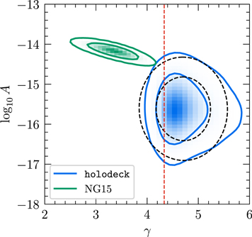
Figure 1. Comparison of the 68% and 95% probability regions for the amplitude and slope of a power-law fit to the observed GWB signal (green contours) and predicted for purely GW-driven SMBHB populations with circular orbits (blue contours; NG15smbh). The black dashed lines represent a 2D Gaussian fit of the blue contours. The vertical red line indicates γ = 13/3, the naive expectation for a GWB produced by a GW-driven SMBHB population (Phinney 2001).
Download figure:
Standard image High-resolution imageThe black dashed contours in Figure 1 show the results of a 2D Gaussian fit to the distribution of ABHB and γBHB values derived from the simulated SMBHB populations (see Equation (A1) in Appendix A for the parameters of this Gaussian distribution). This fitted distribution is what we adopt as a prior distribution for ABHB and γBHB in all parts of the analysis described in this paper.
5. GWB Signals from New Physics
In this section, we discuss the GWB produced by various new-physics models and investigate each model alone and in combination with the SMBHB signal as a possible explanation of the observed GWB signal. For each model, we give a brief review of the mechanism behind the GWB production and discuss the parameterization of its signal prediction. We report the reconstructed posterior distributions of the model parameters and compute the Bayes factors against the baseline SMBHB interpretation. In Figure 2, we show a summary of these Bayes factors; in Figure 3, we present median reconstructed GWB spectra in the PTA band for a number of select new-physics models; and in Figure 4, we show similar median reconstructed GWB spectra in the broader landscape of present and future GW experiments.
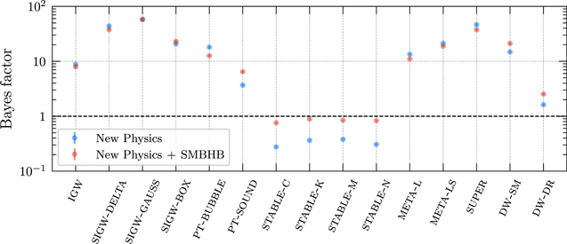
Figure 2. Bayes factors for the model comparisons between the new-physics interpretations of the signal considered in this work and the interpretation in terms of SMBHBs alone. Blue points are for the new physics alone, and red points are for the new physics in combination with the SMBHB signal. We also plot the error bars of all Bayes factors, which we obtain following the bootstrapping method outlined in Section 3.2. In most cases, however, these error bars are small and not visible.
Download figure:
Standard image High-resolution image
Figure 3. Median GWB spectra produced by a subset of the new-physics models, which we construct by mapping our model parameter posterior distributions to h2ΩGW distributions at every frequency f (see Appendix B for more details and Figures 19 and 20 for the models not included here). We also show the periodogram for an HD-correlated free spectral process (gray violins) and the GWB spectrum produced by an astrophysical population of inspiraling SMBHBs with the parameters ABHB and γBHB fixed at the central values μ BHB of the 2D Gaussian prior distribution specified in Equation (A1) (black dashed line).
Download figure:
Standard image High-resolution image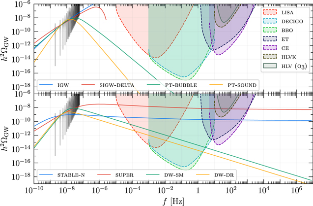
Figure 4. Same as Figure 3, but for a different selection of models and showing a larger frequency range. The solid lines represent median GWB spectra for a subset of new-physics models (see Appendix B for more details), the gray violins correspond to the posteriors of an HD-correlated free spectral reconstruction of the NANOGrav signal, and the shaded regions indicate the power-law-integrated sensitivity (Thrane & Romano 2013) of various existing and planned GW interferometer experiments: LISA (Amaro-Seoane et al. 2017), DECIGO (Kawamura et al. 2011), BBO (Crowder & Cornish 2005), Einstein Telescope (ET; Punturo et al. 2010), Cosmic Explorer (CE; Reitze et al. 2019), the HLVK detector network (consisting of aLIGO in Hanford and Livingston (Aasi et al. 2015), aVirgo (Acernese et al. 2015), and KAGRA (Akutsu et al. 2019)) at design sensitivity, and the HLV detector network during the third observing run (O3). All sensitivity curves are normalized to a signal-to-noise ratio of unity and, for planned experiments, an observing time of 1 yr. For the HLV detector network, we use the O3 observing time. Different signal-to-noise thresholds ρthr and observing times tobs can be easily implemented by rescaling the sensitivity curves by a factor of  . More details on the construction of the sensitivity curves can be found in Schmitz (2021). We emphasize that models whose median GWB spectrum exceeds the sensitivity of existing experiments are not automatically ruled out. This applies, e.g., to cosmic superstrings (super) and the O3 sensitivity of the HLV detector network. Typically, no single GWB spectrum in a given model will coincide with the median GWB spectrum, which is constructed from distributions of h2ΩGW values at any given frequency. Therefore, if the median GWB spectrum is in conflict with existing bounds, typically only some regions in the model parameter space will be ruled out, while others remain viable (see, e.g., Figure 11 for the super model). Finally, note that any primordial GWB signal is subject to the upper limit on the amount of dark radiation in Equation (23), which requires the total integrated GW energy density to remain smaller than
  (see Section 5.1).
Download figure:
Standard image High-resolution imageAs discussed in Section 4 and in more detail in NG15smbh, there is a mild tension between the NG15 data and the predictions of SMBHB models. The models generally prefer a weaker and less blue-tilted h2ΩGW spectrum than the data. This discrepancy presents an opportunity for new-physics models to fit the data better than the conventional SMBHB signal. Eventually, this tension may grow to the point of giving strong evidence for new physics, or it may be resolved with better modeling and more data. Specifically, models of SMBHB evolution with a significant coupling between binaries and their local environment could lead to a signal that better aligns with the data and reduce the evidence for new physics. For all these reasons, we caution against overinterpreting the observed evidence in favor of some of the new-physics models discussed in the following sections.
5.1. Cosmic Inflation
5.1.1. Model Description
Cosmic inflation denotes a stage of exponential expansion in the early universe that provides an explanation for the initial conditions of big bang cosmology (Liddle & Lyth 2009). At the level of the background expansion, inflation accounts for the size, homogeneity, isotropy, and flatness of the observable universe on cosmological scales; at the level of perturbations, it provides the seeds for structure formation in the form of primordial density fluctuations. In the standard scenario of inflation, these primordial perturbations are sourced by scalar quantum vacuum fluctuations of the spacetime metric and inflaton field, which are first stretched to superhorizon scales during inflation and then reenter the horizon in the form of classical density perturbations after inflation. In addition to scalar perturbations, inflation also leads to the amplification of tensor perturbations of the metric, which reenter the horizon in the form of stochastic GWs after inflation. These primordial or inflationary GWs (IGWs; Grishchuk 1974; Starobinsky 1979; Rubakov et al. 1982; Fabbri & Pollock 1983; Abbott & Wise 1984) represent a prime GW signal from the early universe. For earlier work on the IGW interpretation of the signal in recent PTA data sets, see Vagnozzi (2021), Kuroyanagi et al. (2021), and Benetti et al. (2022).
IGWs leave an imprint in the temperature and polarization anisotropies of the cosmic microwave background (CMB) whose relative strength compared to the contributions from scalar perturbations is quantified in terms of the tensor-to-scalar ratio, r. For the simplest type of inflation—standard single-field slow-roll inflation—the h2ΩGW spectrum is red-tilted at CMB scales, with the tensor spectral index nt being given by the so-called consistency relation, nt = − r/8 < 0. Meanwhile, r is bounded from above by current CMB observations, r ≤ 0.036 at 95% C.L. (Ade et al. 2021). A vanishing tensor spectral index, nt ≈ 0, would imply an upper bound on the GW energy density spectrum of ΩGW h2 ∼ 10−16 at PTA frequencies, rendering any detection of an IGW signal in PTA observations hopeless. This conclusion, however, only applies to the standard case of single-field slow-roll inflation. Nonminimal scenarios may have significantly better detection prospects.
We remain agnostic about the microphysics of inflation and restrict ourselves to a model-independent analysis, in which we parameterize the IGW signal in terms of four parameters: the tensor-to-scalar ratio r and tensor spectral index nt at the CMB pivot scale, fCMB = 0.05 Mpc−1/(2π a0) ≃ 7.73 × 10⁻¹⁷ Hz, which quantify the efficiency and scale dependence of GW production during inflation, and the reheating temperature Trh and the number of e-folds during reheating Nrh, which describe the reheating process after inflation. Here the factor a0 in the expression for fCMB denotes the present value of the cosmological scale factor a(t) in the Robertson–Walker metric; in our convention, a0 = 1.
We do not impose the standard consistency relation between r and nt
; instead, we allow both parameters to vary independently across large prior ranges, ![${\mathrm{log}}_{10}r\in [-40,0]$](https://content.cld.iop.org/journals/2041-8205/951/1/L11/revision5/apjlacdc91ieqn37.gif) and nt
∈ [0, 6]. We note that blue values of the tensor spectral index can be generated, e.g., from axion–vector dynamics during inflation (Anber & Sorbo 2012; Cook & Sorbo 2012; Namba et al. 2016; Dimastrogiovanni et al. 2017; Caldwell & Devulder 2018) or in other nonminimal inflation models (see Piao & Zhang 2004; Satoh & Soda 2008; Kobayashi et al. 2010; Endlich et al. 2013; Fujita et al. 2019 for an incomplete list).
and nt
∈ [0, 6]. We note that blue values of the tensor spectral index can be generated, e.g., from axion–vector dynamics during inflation (Anber & Sorbo 2012; Cook & Sorbo 2012; Namba et al. 2016; Dimastrogiovanni et al. 2017; Caldwell & Devulder 2018) or in other nonminimal inflation models (see Piao & Zhang 2004; Satoh & Soda 2008; Kobayashi et al. 2010; Endlich et al. 2013; Fujita et al. 2019 for an incomplete list).
Similarly, we allow for more flexibility for Trh and Nrh than in the standard treatment of single-field slow-roll inflation. To illustrate this point, note that the number of e-folds during reheating, Nrh, can be written as (Liddle & Lyth 2009)

where Hend is the Hubble rate at the end of inflation, wrh is the equation-of-state parameter during reheating, MPl ≃ 2.44 × 10¹⁸ GeV is the reduced Planck mass, and  is defined below. We assume for definiteness that reheating is dominated by the coherent oscillations of the inflaton field, such that the equation of state is equivalent to the one of pressureless dust (i.e., matter), wrh = 0. In typical models of single-field slow-roll inflation, one can often approximate Hend by the Hubble rate at the time of CMB horizon exit during inflation, such that

where Hnaive is fixed by the tensor-to-scalar ratio r and the amplitude of the primordial scalar power spectrum, As ≃ 2.10 × 10⁻⁹ (Aghanim et al. 2020),

However, we already assume nonminimal dynamics in order to motivate a strongly blue-tilted h2ΩGW spectrum, so there is no reason why we should make use of this approximation. In our analysis, we therefore treat Hend and correspondingly Nrh as independent parameters and do not fix them in terms of r and Trh as in Equations (15) and (16). This flexibility provides us with more parametric freedom that we can use in order to ensure that the IGW signal does not violate constraints on the amplitude of the stochastic GWB set by the LIGO–Virgo–KAGRA (LVK) Collaboration (Abbott et al. 2021a) and on the amount of dark radiation, i.e., the effective number of neutrino species, Neff, inferred from big bang nucleosynthesis (BBN) and the CMB (Pisanti et al. 2021; Yeh et al. 2021). As for the latter constraint, we specifically work with ΔNeff = ρDR/ρν
, where ρDR is the energy density of dark radiation (i.e., the integrated GW energy density in the context of the igw model) and ρν
denotes the energy density of a single neutrino species. ΔNeff characterizes the excess energy in radiation beyond the SM expectation (i.e., dark radiation) after neutrino decoupling and e+
e− annihilation,  , where
  (Bennett et al. 2021).
Under the assumptions outlined above, we are able to model the IGW spectrum at PTA frequencies as
Here  is the current radiation energy density per relativistic degree of freedom, in units of the critical (closure) density,
  counts the effective number of relativistic degrees of freedom contributing to the radiation entropy today, and g*(f) and g*,s
(f) denote the effective numbers of relativistic degrees of freedom in the early universe when GWs with comoving wavenumber k = 2π
a0
f reentered the Hubble horizon after inflation. In order to evaluate g*(f) and g*,s
(f), we use the numbers of relativistic degrees of freedom as functions of temperature tabulated in Saikawa & Shirai (2020), g*(T) and g*,s
(T), in combination with the standard temperature–frequency relation in ΛCDM (i.e., the cosmological Lambda cold dark matter SM) that follows from the condition k = a(T)H(T) at the time of horizon reentry. In the remainder of this paper, whenever we need g* or g*,s
in a different part of our analysis, we will use the same functions g*(f), g*,s
(f), g*(T), and g*,s
(T).
counts the effective number of relativistic degrees of freedom contributing to the radiation entropy today, and g*(f) and g*,s
(f) denote the effective numbers of relativistic degrees of freedom in the early universe when GWs with comoving wavenumber k = 2π
a0
f reentered the Hubble horizon after inflation. In order to evaluate g*(f) and g*,s
(f), we use the numbers of relativistic degrees of freedom as functions of temperature tabulated in Saikawa & Shirai (2020), g*(T) and g*,s
(T), in combination with the standard temperature–frequency relation in ΛCDM (i.e., the cosmological Lambda cold dark matter SM) that follows from the condition k = a(T)H(T) at the time of horizon reentry. In the remainder of this paper, whenever we need g* or g*,s
in a different part of our analysis, we will use the same functions g*(f), g*,s
(f), g*(T), and g*,s
(T).
The inflationary dynamics give rise to the primordial tensor power spectrum  , while the transfer function
  accounts for the redshifting behavior of GWs after horizon reentry. In our analysis, we assume a constant tensor spectral tilt (i.e., zero running of nt
) from CMB to PTA frequencies, such that
accounts for the redshifting behavior of GWs after horizon reentry. In our analysis, we assume a constant tensor spectral tilt (i.e., zero running of nt
) from CMB to PTA frequencies, such that
Meanwhile, the only relevant contribution to  in the PTA band corresponds to the transfer function that connects the radiation-dominated era to reheating,
Here the fit function in the denominator of this expression is taken from Kuroyanagi et al. (2015, 2021) and describes the spectral turnover,  , at frequencies around f ∼ frh, which marks the end of the reheating period,
with  and
and  and the present-day CMB temperature T0 ≃ 2.73 K (Fixsen 2009). The Heaviside theta function in Equation (19) denotes the endpoint of the IGW spectrum at f = fend, which marks the end of inflation and hence the onset of reheating,
For fixed Trh, the frequency fend is solely controlled by Hend, which follows from our choice of Nrh according to Equation (14) (recall that we set wrh = 0). In our MCMC analysis, we do not sample over fend, since its precise value does not affect the shape of the IGW spectrum in the PTA band and hence the quality of our fit. Instead, we constrain its maximally allowed value (i.e., Nrh) after identifying the viable region in the r–nt
–Trh parameter space, in order to make sure that the IGW spectrum does not violate the Neff and LVK bounds. The frequency frh, on the other hand, can easily fall into the PTA band: from Equation (20), we have  . Therefore, we sample the reheating temperature in a symmetric interval around Trh = 1 GeV extending down to temperatures relevant for BBN, TBBN ∼ 1 MeV. That is, we work with the log-uniform prior
 ![${\mathrm{log}}_{10}\left({T}_{\mathrm{rh}}/1\,{\rm{GeV}}\right)\in \left[-3,+3\right]$](https://content.cld.iop.org/journals/2041-8205/951/1/L11/revision5/apjlacdc91ieqn50.gif) .
.
5.1.2. Results and Discussion
We now discuss the outcome of our Bayesian fit analysis. First, we note that the igw model fits the NG15 data slightly better than the baseline smbhb model. This is evident from the Bayes factor that we find for the igw versus smbhb model comparison,  (mean value and one standard deviation), and simply follows from the larger parametric freedom of the igw model. Both the igw and smbhb models basically correspond to a power-law approximation of the GW spectrum. However, in the case of the igw model, the parameters controlling this power law are drawn from prior distributions that allow for a larger amplitude and a steeper slope of the spectrum, which improves the quality of the fit. Meanwhile, the combined GW spectrum from inflation with an additional SMBHB signal on top compared to the smbhb model alone results in a Bayes factor of
  . We thus observe a slight decrease in the Bayes factor, which accounts for the fact that adding the SMBHB signal on top of the IGW signal does not improve the quality of fit but merely increases the prior volume compared to the igw model.
The reconstructed posterior distributions for the parameters of the igw model and its igw+smbhb extension are shown in Figure 5. 81 For both models, we find a strong covariance between the spectral index nt and the tensor-to-scalar ratio r, which is approximately fit by

and which can be explained as follows: the igw interpretation of the PTA signal requires the primordial tensor power spectrum  to take values of
  at nanohertz frequencies. This requirement fixes the parameter combination
  in Equation (18) and thus allows us to estimate the coefficients in Equation (22) as
  and
and  , respectively, where we used fPTA = 1 nHz and
  .
.

Figure 5. Reconstructed posterior distributions for the parameters of the igw (blue) and igw+smbhb (red) models. On the diagonal of the corner plot, we report the 1D marginalized distributions together with the 68% Bayesian credible intervals (vertical lines), while the off-diagonal panels show the 68% (darker) and 95% (lighter) Bayesian credible regions in the 2D posterior distributions. We construct all credible intervals and regions by integrating over the regions of highest posterior density. The gray shaded regions are strongly disfavored by the NG15 data, as they result in a K ratio of less than 1/10 (see Equation (10)). The black shaded region results in a violation of the Neff bound in Equation (23) (see Appendix C.1 and Figure 22), assuming Nrh = 0 (solid line), Nrh = 5 (dashed line), and Nrh = 10 (dotted line). Figure 21 in Appendix C.1 shows an extended version of this plot that includes the SMBHB parameters ABHB and γBHB.
Download figure:
Standard image High-resolution imageIn addition to the strong covariance between nt
and r, we note that the posterior probabilities of both parameters exhibit a bimodal distribution for both igw and igw+smbhb. In the 2D distributions of the parameter pairs  and
and  , this bimodality is accompanied by an approximate reflection symmetry with respect to the points
  and
and  , respectively. These features of the corner plot in Figure 5 indicate that the igw model can operate in two regimes: for Trh ≫ 1 GeV, the reference frequency frh is larger than the frequencies in the PTA band, and the GW spectrum seen by NANOGrav is composed of tensor modes that reentered the horizon during the radiation-dominated era. For Trh ≪ 1 GeV, on the other hand, frh can be pushed below PTA frequencies, and the GW spectrum in the PTA band is composed of tensor modes that reentered the horizon during reheating after inflation. In the first case, the tilt of the spectrum is directly given by nt
; in the second case, it corresponds to nt
− 2. Clearly, the mirror symmetry in the 2D distributions of
, respectively. These features of the corner plot in Figure 5 indicate that the igw model can operate in two regimes: for Trh ≫ 1 GeV, the reference frequency frh is larger than the frequencies in the PTA band, and the GW spectrum seen by NANOGrav is composed of tensor modes that reentered the horizon during the radiation-dominated era. For Trh ≪ 1 GeV, on the other hand, frh can be pushed below PTA frequencies, and the GW spectrum in the PTA band is composed of tensor modes that reentered the horizon during reheating after inflation. In the first case, the tilt of the spectrum is directly given by nt
; in the second case, it corresponds to nt
− 2. Clearly, the mirror symmetry in the 2D distributions of  and
and  is not exact. At the level of the GW spectrum, it is explicitly broken by the frequency dependence of g* and g*,s
, as well as by the nontrivial shape of the transfer function in Equation (19).
is not exact. At the level of the GW spectrum, it is explicitly broken by the frequency dependence of g* and g*,s
, as well as by the nontrivial shape of the transfer function in Equation (19).
At small or large values of the reheating temperature, the posterior distributions develop approximately flat directions along the Trh axis at  in the large-Trh regime and at
  in the small-Trh regime. This behavior is broadly consistent with the linear fit in Equation (22), the reflection symmetry discussed above, and the fact that, past a certain point, raising or lowering Trh no longer influences the shape of the GW signal in the PTA band. A tensor index of nt
= 2 at large Trh, moreover, corresponds to an index γ = 3 in the timing residual PSD, which is among the best-fitting values—see the 2D posterior for A and γ in Figure 1. The same conclusion holds at low Trh, where γ = 3 is mapped onto nt
− 2 = 2.
in the small-Trh regime. This behavior is broadly consistent with the linear fit in Equation (22), the reflection symmetry discussed above, and the fact that, past a certain point, raising or lowering Trh no longer influences the shape of the GW signal in the PTA band. A tensor index of nt
= 2 at large Trh, moreover, corresponds to an index γ = 3 in the timing residual PSD, which is among the best-fitting values—see the 2D posterior for A and γ in Figure 1. The same conclusion holds at low Trh, where γ = 3 is mapped onto nt
− 2 = 2.
Finally, we derive the Neff and LVK bounds on the igw parameter space. For the Neff bound, the GW spectrum, integrated from BBN scales to the cutoff frequency fend, must not exceed a certain upper limit that is set by the allowed amount of extra relativistic degrees of freedom at the time of BBN and recombination,
Here fBBN ∼ 10−12 Hz refers to tensor modes that reentered the Hubble horizon around the onset of BBN at T ∼ 10−4 GeV (Caprini & Figueroa 2018), and  denotes the upper limit on the amount of dark radiation. For definiteness, we set fBBN = 10−12 Hz and
  in our analysis; the precise
  value at 95% confidence level varies across different combinations of data sets (Pisanti et al. 2021; Yeh et al. 2021). For given values of the parameters Trh, r, and nt
, we can then ask whether there is a cutoff frequency
value at 95% confidence level varies across different combinations of data sets (Pisanti et al. 2021; Yeh et al. 2021). For given values of the parameters Trh, r, and nt
, we can then ask whether there is a cutoff frequency  that leads to the saturation of the inequality in Equation (23). If this is the case,
  yields an upper bound on the allowed number of e-folds during reheating,
  , according to Equations (14) and (21). A second constraint on Nrh follows from the LVK bound on the amplitude of the GWB (Abbott et al. 2021a),

assuming a flat GW spectrum. For a power-law spectrum,  with α = nt
− 2 at f ≫ frh, this bound can be generalized following (Kuroyanagi et al. 2015, 2021)
with α = nt
− 2 at f ≫ frh, this bound can be generalized following (Kuroyanagi et al. 2015, 2021)
which approximately holds if α ≪ 5/2. For given values of Trh, r, and nt
, we can then evaluate  at flvk and check whether it exceeds the LVK bound. If so, we place an upper bound on Nrh by demanding that
  (the lower end of the LVK frequency band).
The outcome of our analysis is shown Figure 22 in Appendix C.1. In both plots of this figure, the dependence on the tensor-to-scalar ratio r is eliminated by means of the linear relation in Equation (22). In the left panel of Figure 22, we present contour lines of  derived from the Neff bound and the LVK bound, respectively. In a realization of the igw model with a given duration of reheating, these contour lines can be thought of as bounds on the Trh–nt
parameter plane—for fixed Nrh, the regions with
derived from the Neff bound and the LVK bound, respectively. In a realization of the igw model with a given duration of reheating, these contour lines can be thought of as bounds on the Trh–nt
parameter plane—for fixed Nrh, the regions with  are excluded. We find that the Neff bound rules out most values of the spectral index nt
in the large-Trh regime. At the same time, large regions of parameter space remain viable as long as
are excluded. We find that the Neff bound rules out most values of the spectral index nt
in the large-Trh regime. At the same time, large regions of parameter space remain viable as long as  . In fact, away from the region where
  turns negative, our upper bound is typically rather large,
  , and hence easy to satisfy in realistic models of reheating, where
  . In the right panel of Figure 22, we compare our result to the naive expectation
  in single-field slow-roll inflation with a nearly constant Hubble rate (see Equation (15)). Across large parts of parameter space, we find that
  assumes unrealistically large values,
  .
.
In Figure 5, we highlight the constraints on Trh and nt (as well as Trh and r) that we deduce from the Neff bound assuming Nrh values of Nrh = 0, 5, and 10. Here the constraints for Nrh = 0 correspond to the assumption of instantaneous reheating after inflation and hence represent the most conservative bound on the Trh–nt parameter plane. A longer duration of reheating results in tighter constraints on Trh and nt , as illustrated by the contours for Nrh = 5 and 10. For an even larger number of e-folds during reheating, see Figure 22 in Appendix C.1.
In view of Figures 5 and 22, we conclude that the igw model is indeed capable of fitting the NANOGrav signal across large regions in parameter space. An interesting viable scenario consists, e.g., of a large tensor spectral index, nt ∼ 3 ⋯ 4, a tiny tensor-to-scalar ratio, r ∼ 10−(23⋯16), a low reheating temperature, Trh ∼ 10−(3⋯0) GeV, and a moderate number of e-folds during reheating, Nrh ≲ 20. It remains to be seen whether it is possible to identify explicit microscopic models that realize inflation in this parametric regime.
5.2. Scalar-induced Gravitational Waves
5.2.1. Model Description
The amplitude of the primordial scalar power spectrum is well measured by CMB observations, As ≃ 2.10 × 10⁻⁹ at the CMB pivot scale kCMB = 0.05 Mpc−1 (Aghanim et al. 2020). If we naively extrapolate this value down to smaller scales, assuming a fixed and slightly red-tilted h2ΩGW spectrum with index ns ∼ 0.96, we are led to conclude that there must be increasingly less power in scalar perturbations on shorter scales. This conclusion can, however, be easily avoided in models that deviate from the standard picture of single-field slow-roll inflation giving rise to a nearly scale-invariant spectrum of scalar perturbations. A prominent example, among many other mechanisms, consists in a stage of inflation close to an inflection point in the scalar potential, which readily amplifies the scalar perturbations leaving the horizon (see, e.g., Garcia-Bellido & Ruiz Morales 2017; Ballesteros & Taoso 2018; Ezquiaga et al. 2018). An enhanced scalar power spectrum at small scales is, therefore, a viable possibility. Moreover, it promises a rich phenomenology with regard to the production of GWs and potentially the origin of primordial black holes (PBHs; Carr et al. 2016; Garcia-Bellido et al. 2016; Inomata et al. 2017a; Inomata & Nakama 2019; Wang et al. 2019; Escrivà et al. 2022b). The possibility of having PBH formation in models of single-field inflation is the subject of ongoing debate (Kristiano & Yokoyama 2022, 2023; Choudhury et al. 2023a, 2023b, 2023c; Firouzjahi & Riotto 2023; Riotto 2023a, 2023b). Below, we comment on the implications of this debate for our PBH-related parameter bounds.
In cosmological perturbation theory, scalar and tensor perturbations evolve independently at linear order. Starting at second order, however, they are coupled, which means that large first-order scalar perturbations can act as a source of second-order tensor perturbations. We refer to these tensor perturbations, which are produced as soon as the enhanced scalar perturbations reenter the Hubble horizon after inflation, as SIGWs (Matarrese et al. 1993, 1994, 1998; Mollerach et al. 2004; Ananda et al. 2007; Baumann et al. 2007; see Domènech 2021 for a review and more details on the history of SIGWs). At the same time, large overdensities in the tail of the distribution of scalar perturbations can collapse into PBHs upon horizon reentry. This PBH production mechanism thus results in a PBH population whose properties are strongly correlated with the spectral shape of the SIGW signal, as both phenomena are controlled by the scalar spectrum generated during inflation (Yuan & Huang 2021a). For earlier works on the PBH/SIGW interpretation of the signal in recent PTA data sets, see Vaskonen & Veermäe (2021), De Luca et al. (2021), and Kohri & Terada (2021). For earlier Bayesian searches for an SIGW signal in PTA data sets, see Chen et al. (2020), Bian et al. (2021), Zhao & Wang (2022), Yi & Fei (2023), and Dandoy et al. (2023), and for a search in LVK data, see Romero-Rodriguez et al. (2022).
In our analysis, we consider SIGWs in the PTA band and model the associated GW spectrum as follows:
where the first three factors account for the cosmological redshift as in Equation (17) and the last factor denotes the GW spectrum at the time of production, which we assume to be during the radiation-dominated era,

The present-day GW frequency is related to the comoving wavenumber by  ,
,  denotes the primordial spectrum of the comoving curvature perturbation
  , and the integration kernel
  is given by (Espinosa et al. 2018; Kohri & Terada 2018; Pi & Sasaki 2020; Gong 2022)

The expression in Equation (27) illustrates the dependence of the SIGW signal on the scalar input spectrum; in particular, it shows that  scales as
  . We stress that the expression in Equation (27) assumes Gaussian perturbations, whose statistics are fully described by the power spectrum
  . We do not consider any non-Gaussian contributions to the primordial scalar power spectrum in our analysis. The impact of non-Gaussianities on the SIGW signal was studied in Nakama et al. (2017), Cai et al. (2019), Unal (2019), Atal et al. (2019), Yuan & Huang (2021b), Atal & Domènech (2021), Adshead et al. (2021), and Ferrante et al. (2023).
To remain as model-independent as possible, we refrain from choosing a particular inflation model capable of generating an enhanced spectrum  . Instead, we ignore the microphysics of inflation and work with three characteristic templates for
  that reflect the range of possibilities that one may expect in realistic models. Specifically, we consider the following templates:
sigw-delta: Sharp spectral feature in  modeled by a Dirac delta function in logarithmic k space,

sigw-Gauss: Broad spectral feature in  modeled by a Gaussian peak in logarithmic k space,
sigw-box: Flat and continuous spectral feature in  modeled by a box function in logarithmic k space,

Note that the Gaussian power spectrum in logarithmic k space that we assume in the sigw-Gauss model corresponds to a lognormal power spectrum in linear k space. As evident from the above expressions, sigw-delta represents a two-parameter model, while sigw-Gauss and sigw-box are three-parameter models. Our prior choices for the respective parameters are listed in Table 3 in Appendix A, where we use again  to convert from wavenumber to frequency. For a given set of parameter values, we are then able to use the scalar power spectrum in Equation (29), Equation (30), or Equation (31) to evaluate the integrals in Equation (27) and compute the GW spectrum. For sigw-Gauss and sigw-box, the integration needs to be carried out numerically; for sigw-delta, we can resort to the exact analytical expression provided in Wang et al. (2019) and Yuan & Huang (2021a).
5.2.2. Results and Discussion
We now turn to the outcome of our Bayesian fit analysis. Compared to the igw model discussed in Section 5.1, we obtain even larger Bayes factors, indicating that SIGWs tend to provide an even better fit of the NG15 data than IGWs. Specifically, we obtain  ,
,  , and
, and  for sigw-delta, sigw-Gauss, and sigw-box, respectively, and
  ,
,  , and
, and  for sigw-delta+smbhb, sigw-Gauss+smbhb, and sigw-box+smbhb, respectively (see Figure 2). This improvement in the quality of the fit reflects the fact that the SIGW spectra deviate from a pure power law and thus manage to provide a better fit across the whole frequency range probed by NANOGrav (see Figure 3). For sigw-delta, we observe again that adding the SMBHB signal does not improve the quality of the fit. The larger prior volume of sigw-delta+smbhb compared to sigw-delta therefore results in a slight decrease of the Bayes factor. For the other two SIGW models, the Bayes factors remain more or less the same, within the statistical uncertaintity of our bootstrapping analysis.
The reconstructed posterior distributions for all SIGW models under consideration are shown in Figures 6 and 7. Our first conclusion in view of these results is that a successful explanation of the NANOGrav signal in terms of SIGWs requires the primordial scalar power spectrum to have a large amplitude A. We can quantify this statement in terms of the lower limits of the 95% Bayesian credible intervals for A that we obtain from integrating the corresponding 1D marginalized posteriors over the regions of highest posterior density: for sigw-delta, sigw-Gauss, and sigw-box, we respectively find  ,
,  , and
, and  . At the same time, the enhanced power in scalar perturbations must be localized at the right scales, so that the resulting SIGW signal falls into the PTA band. This requirement leads to bounds on the frequencies
  ,
,  , and f* that can be read off from Figures 6 and 7 and that are summarized in Table 4.

Figure 6. Same as in Figure 5, but for the sigw-box model. The regions above the teal contour lines labeled fPBH = 1 lead to the overproduction of PBHs, according to our analysis in Appendix C.2; however, see text for more discussion. Figure 23 in Appendix C.2 shows an extended version of this plot that includes the SMBHB parameters ABHB and γBHB.
Download figure:
Standard image High-resolution image
Figure 7. Same as in Figure 6, but for the sigw-delta (left panel) and sigw-Gauss (right panel) models. The solid and dashed teal contour lines labeled fPBH = 1 in the right panel indicate the PBH bound for Δ = 1 and Δ = 2, respectively. Figure 24 in Appendix C.2 shows extended versions of the two plots that include the SMBHB parameters ABHB and γBHB.
Download figure:
Standard image High-resolution imageA notable feature in this context is that the posterior distributions for  ,
,  , and f* all extend to large frequencies, much beyond the upper limit of the NANOGrav band. The reason for this is that the NG15 data are best fit by the low-frequency tail of the SIGW spectrum (see Figure 19). Beyond the NANOGrav band, the SIGW spectrum keeps increasing until it reaches its maximal value at f ≫ 1 nHz. This observation also explains the flat directions in the 2D posterior distribution for A and
  in Figure 6 and the 2D posterior distributions for A and f* in Figure 7. A simultaneous increase in A and
  or f* along these flat directions moves the peak in the GW spectrum to higher frequencies, but it preserves the shape of the low-frequency tail in the PTA band and hence does not affect the quality of the fit.
We also observe that the 2D posterior distributions for A and f* for sigw-delta and sigw-Gauss are roughly similar to each other, with the distribution for the sigw-Gauss model being slightly broader. This result is consistent with the fact that sigw-delta and sigw-Gauss are nested models; sigw-delta can be obtained from sigw-Gauss in the limit Δ → 0. The slightly broader posterior distribution for A and f* in the right panel of Figure 7 thus reflects the extra dimension in the parameter space of the sigw-Gauss model and the additional parametric freedom that comes with it.
Finally, we comment on the bounds on the parameter space of the three SIGW models. As in the case of the igw model, we identify regions of the parameter space where the K ratio in Equation (10) falls below 1/10. In these regions, which are shaded in gray in Figure 7 and labeled NG15, adding the SIGW contribution to the GW signal leads to much worse agreement with the data than in the case of no SIGW contribution at all. In fact, parameter points in these regions lead to an SIGW signal that exceeds the observed signal—in other words, the gray shaded regions are ruled out because they result in too strong of an SIGW signal. For sigw-box, we are not able to place a K-ratio bound on the 2D parameter space spanned by A and  , because we additionally marginalize over
  . That is, for any pair of values of A and
  , the SIGW signal can be made arbitrarily small if we choose
  close enough to
  .
.
These bounds are an important result of our analysis that is independent of the origin of the NANOGrav signal. They provide valid constraints on the parameter space for both the sigw-delta and sigw-Gauss models, regardless of whether these models contribute to the explanation of the observed GWB. In addition, they are complementary to other existing bounds, in particular, the requirement that the mass density of PBHs produced alongside SIGWs must not exceed the energy density of DM,

where fPBH = ΩPBH/ΩDM denotes the PBH DM fraction integrated over the entire PBH mass spectrum. We provide more details on how we compute fPBH in Appendix C.2; here we simply report our final results in terms of the teal contour lines labeled fPBH = 1 in Figures 6 and 7. For sigw-box, the PBH bound in the A– plane is computed for
  (the lower end of our prior range), and the PBH bound in the A–
 plane is computed for
  (the upper end of our prior range). For sigw-Gauss, we show the PBH bound in the A–f* plane for Δ = 1 (solid contour line) and Δ = 2 (dashed contour line).
In all three cases, we find that the PBH bound is very restrictive, ruling out most of the parameter space favored by the NG15 data. If taken at face value, the PBH bound therefore renders the SIGW interpretation of the NANOGrav signal less likely. However, we stress that the computation of fPBH is very sensitive to various assumptions and numerical steps in the analysis. Slight changes in the computational strategy may result in very different results for fPBH, which is why the results reported in Figures 6 and 7 need to be treated with caution. In view of the large conceptional uncertainty in the computation of fPBH, one needs to be careful not to draw any premature conclusions. At the same time, the PBH bounds in Figures 6 and 7 illustrate that small regions of parameter space do remain viable. In fact, for sigw-delta and sigw-Gauss, it is even possible to realize fPBH = 1 inside the 68% credible regions. That is, along the fPBH = 1 contour lines and inside the 68% credible regions, we find scenarios where SIGWs manage to provide a good fit to the NG15 data and PBHs account for the entire DM in our universe.
In closing, we remark that the above conclusions are endangered by the recent claim of a no-go theorem for PBH formation from single-field inflation (Kristiano & Yokoyama 2022, 2023). Kristiano & Yokoyama (2022, 2023) argue that enhanced scalar perturbations at small scales lead to unacceptably large one-loop corrections to the scalar power spectrum at large scales. In terms of the model parameters discussed in this section, this means that the amplitude A must be small,  otherwise, the loop corrections to the scalar power spectrum will exceed the measured amplitude at CMB scales, As
≃ 2.10 × 10⁻⁹. At present, this claim is subject to an ongoing debate; it is notably challenged by Riotto (2023a, 2023b) and Firouzjahi & Riotto (2023). However, if it should prove to be valid, the requirement of
otherwise, the loop corrections to the scalar power spectrum will exceed the measured amplitude at CMB scales, As
≃ 2.10 × 10⁻⁹. At present, this claim is subject to an ongoing debate; it is notably challenged by Riotto (2023a, 2023b) and Firouzjahi & Riotto (2023). However, if it should prove to be valid, the requirement of  would clash with the lower bounds on A listed above. In this case, one would then have to either give up on the SIGW interpretation of the NANOGrav signal or seek to construct inflation models that evade the arguments of Kristiano & Yokoyama (2022, 2023) and still lead to a large SIGW signal.
5.3. Cosmological Phase Transitions
5.3.1. Model Description
In the cosmological context, first-order phase transitions take place when a potential barrier separates the true and false minima of a scalar field potential. 82 The phase transition is triggered by quantum or thermal fluctuations that cause the scalar field to tunnel through or fluctuate over the barrier, which results in the nucleation of bubbles within which the scalar field is in the true vacuum configuration. If sufficiently large, these bubbles expand in the surrounding plasma where the scalar field still resides in the false vacuum. The expansion and collision of these bubbles (Kosowsky et al. 1992a, 1992b; Kosowsky & Turner 1993; Kamionkowski et al. 1994; Caprini et al. 2008; Huber & Konstandin 2008), together with sound waves generated in the plasma (Giblin & Mertens 2013, 2014; Hindmarsh et al. 2014, 2015), can source a primordial GWB (see Witten 1984; Hogan 1986 for seminal work). 83 For earlier Bayesian searches for a phase transition signal in PTA data, see Arzoumanian et al. (2021) and Xue et al. (2021).
Generally, the GWB produced during the phase transition is a superposition of the bubble and sound-wave contributions. However, if the bubble walls interact with the surrounding plasma, most of the energy released in the phase transition is expected to be converted to plasma motion, causing the sound-wave contribution to dominate the resulting GWB. An exception to this scenario is provided by models in which there are no (or only very feeble) interactions between the bubble walls and the plasma, or by models where the energy released in the phase transition is large enough that the friction exerted by the plasma is not enough to stop the walls from accelerating (runaway scenario). However, determining whether or not the runaway regime is reached is either model dependent or affected by large theoretical uncertainties (see, e.g., Ai et al. 2023; Krajewski et al. 2023; Li et al. 2023, for recent work on this topic). Therefore, in this work, we perform two separate analyses: a sound-wave-only analysis (pt-sound), where we assume that the runaway regime is not reached and sound waves dominate the GW spectrum, and a bubble-collisions-only analysis (pt-bubble), where we assume that the runaway regime is reached and bubble collisions dominate the GW spectrum.
We parameterize the GWB produced by both sound waves and bubble collisions in a model-independent way in terms of the following phase transition parameters:
- 1.T*, the percolation temperature, i.e., the temperature of the universe when ∼34% of its volume has been converted to the true vacuum (Ellis et al. 2019a). For weak transitions, this temperature coincides with the temperature at the time of bubble nucleation, Tn ∼ T*. Conversely, for supercooled transitions, we typically have Tn ≪ T*. Barring the case of extremely strong transitions, α* ⋙ 1 (see below), which we do not consider in this work, T* also determines the reheating temperature after percolation, Trh ∼ T* (Ellis et al. 2019a).
- 2.
- 3.
 , the average bubble separation in units of the Hubble radius at percolation, . For relativistic bubble velocities, which is what we consider in the following, R* is related to the bubble nucleation rate, β, by the relation H*
R* = (8π)1/3
H*/β.
, the average bubble separation in units of the Hubble radius at percolation, . For relativistic bubble velocities, which is what we consider in the following, R* is related to the bubble nucleation rate, β, by the relation H*
R* = (8π)1/3
H*/β.


In addition to the parameters T*, α*, and H* R*, the GWB produced by a phase transition also depends on the velocity of the expanding bubble walls, vw . However, deriving the precise value of this quantity is an open theoretical problem, which depends on model-dependent quantities, such as the strength of the interactions between the bubble walls and the SM plasma. Therefore, in our analysis, we fix the bubble velocity to unity (i.e., the speed of light in natural units). This assumption is well justified for strong phase transitions (Bodeker & Moore 2017), which, realistically, are the only ones that could lead to a detectable signal in our current data. In particular, we fix vw = 1 for both phase transition scenarios that we are interested in, pt-sound and pt-bubble. In the latter case, vw → 1 is automatically implied by the runaway behavior of the phase transition; in the former case, one actually expects a subluminal terminal velocity, vw < 1. In this sense, our decision to fix vw = 1 amounts to the optimistic assumption that this terminal velocity is numerically close to vw = 1. A similar approach is followed by the authors of the LISA review paper (Caprini et al. 2020), who work with vw = 0.95 throughout most of their analysis in the absence of more detailed microphysical calculations. Finally, we point out that the parameterization of the GWB signal in terms of H* R* = (8π)1/3 vw H*/β already absorbs a large part of the dependence on the bubble wall velocity. The remaining vw dependence is mostly contained in the efficiency factor κs (see below). However, in the regime of large α* values, α* ∼ 0.3 ⋯ 10, which turn out to be preferred by the NG15 data (see Figure 8), this dependence is rather weak (see Figure 13 in Espinosa et al. 2010), which justifies again keeping vw fixed.
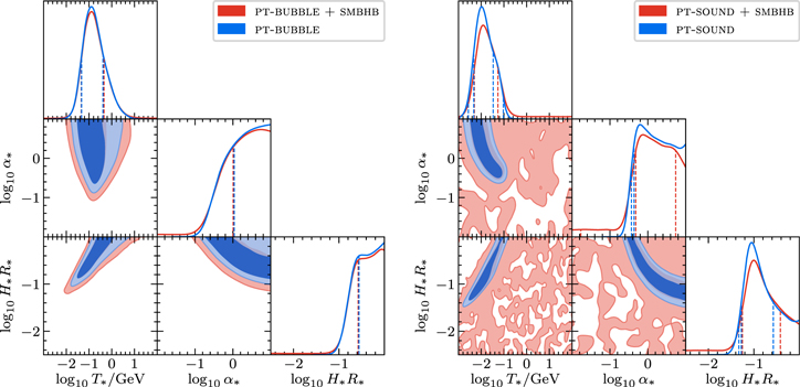
Figure 8. Same as in Figure 5, but for the pt-bubble (left panel) and pt-sound model (right panel). Figure 25 in Appendix C.3 shows the same plots but with the parameter a fixed by causality, a = 3. Figures 26 and 27 in Appendix C.3 show extended versions of the two plots that include the spectral shape parameters a, b, c and the SMBHB parameters ABHB and γBHB.
Download figure:
Standard image High-resolution imageThe GWB spectrum sourced by bubbles and sound waves can be written in terms of these parameters as

Here  (Jinno & Takimoto 2017) and
  (Hindmarsh et al. 2017), the efficiency factor
  (Espinosa et al. 2010) gives the fraction of the released energy that is transferred to plasma motion in the form of sound waves, and
  accounts for the redshift of the GW energy density,
We recall that T0 and H0 denote the photon temperature and Hubble rate today. The degrees of freedom g* and g*,s
in Equation (35) are evaluated at T = T*, and  is the number of degrees of freedom contributing to the radiation entropy at the time of matter–radiation equality. The production of GWs from sound waves stops after a period τsw, when the plasma motion turns turbulent (Ellis et al. 2019a, 2019b, 2020; Guo et al. 2021). In Equation (34), this effect is taken into account by the suppression factor

where the shock formation timescale, τsw, can be written in terms of the phase transition parameters as  , with
 ![${\bar{U}}_{f}^{2}\approx 3{\kappa }_{s}{\alpha }_{* }/[4(1+{\alpha }_{* })]$](https://content.cld.iop.org/journals/2041-8205/951/1/L11/revision5/apjlacdc91ieqn133.gif) (Weir 2018).
(Weir 2018).
The functions  describe the spectral shape of the GWB and are expected to peak at the frequencies
where the values of the peak frequencies at the time of GW emission are given by  (Jinno & Takimoto 2017) and
  (Hindmarsh et al. 2017). In passing, we mention that the numerical factors in these estimates may still change in the future, as our understanding of cosmological phase transitions improves. However, at the level of our Bayesian fit analysis, changes in these prefactors can be absorbed in the temperature scale T*, which in its role as an independent fit parameter only controls the peak frequencies in Equation (37). A similar argument applies to the numerical factors in Equations (33) and (34): changes in these prefactors can always be absorbed in a rescaled version of the fit parameter α*, which only appears in the expressions for the peak amplitudes of the GWB signal.
The shape of the spectral functions can be usually approximated with a broken power law of the form

Here a and b are two real and positive numbers that give the slope of the spectrum at low and high frequencies, respectively; c parameterizes the width of the peak. The normalization constant,  , ensures that the logarithmic integral of
  is normalized to unity and is given by

where n = (a + b)/c and Γ denotes the gamma function. While the values of the coefficients a, b, and c can in principle be estimated from numerical simulations, we allow them to float within the prior ranges given in Table 3. These prior ranges were chosen to roughly reflect the typical uncertainties of numerical simulations and any possible model dependency of these coefficients (see, e.g., Hindmarsh et al. 2017, 2021; Cutting et al. 2018, 2021; Lewicki & Vaskonen 2020, 2021). 84
5.3.2. Results and Discussion
The reconstructed posterior distributions for the parameters α*, T*, and H* R* of the pt-sound and pt-bubble models are reported in Figure 8, both for the case where the phase transition is assumed to be the only source of GWs (blue contours) and for the scenario where we consider the superposition of the phase transition and SMBHB signals (red contours). 85 Corner plots including the posterior distributions for the spectral shape parameters a, b, c and SMBHB parameters ABHB and γBHB are reported in Figures 26 and 27 in Appendix C.3.
In all analyses, the data prefer a relatively strong and slow phase transition. Specifically, for pt-bubble, we find α* > 1.1 (0.29) and H* R* > 0.28 (0.14) at the 68% (95%) credible level. When the SMBHB signal is added on top of the GWB predicted by pt-bubble, we find α* > 1.0 (0.23) and H* R* > 0.26 (0.11) at the 68% (95%) credible level. For the pt-sound model, we find α* > 0.42 (0.37) and H* R* ∈ [0.053, 0.27] ([0.046, 0.89]) at the 68% (95%) credible level. Including the SMBHB signal on top of the one predicted by pt-sound, we find α* ∈ [0.46, 5.4] (>0.16) and H* R* ∈ [0.054, 0.35] (>0.0015) at the 68% (95%) credible level.
As can be seen in Figure 3, for both phase transition models, the reconstructed GWB spectrum tends to peak around the higher frequency bins and fit the signal in the lower frequency bins with the left tail of the spectrum. Specifically, for the pt-bubble model we find T* ∈ [0.047, 0.41] ([0.023, 1.75]) GeV at the 68% (95%) credible level, whereas for the pt-sound model we get T* ∈ [4.7, 33] ([2.7, 93]) MeV at the 68% (95%) credible level. The shift between these T* intervals is partially explained by the different numerical factors in the frequencies  and
and  (see Equation (37)). As explained below Equation (37), any change in these numerical factors can be reabsorbed in a redefinition of the fit parameter T*.
The inclusion of the SMBHB signal, by adding power to the lowest frequency bins, allows the T* posterior for the pt-sound model to extend to higher values. In this case, we find that T* ∈ [4.9, 50] ([0.8, 2 × 10⁶]) MeV at the 68% (95%) credible level. Here the increase in the 68% upper limit is reflected in the slight shift between the red and blue dashed vertical lines in the 1D marginalized posterior distribution for T* in the right panel of Figure 8. The drastic increase in the 95% upper limit, on the other hand, is related to the fact that adding the SMBHB signal to the GWB results in a flat plateau region in the posterior distribution of the pt-sound model parameters where the NANOGrav signal is mostly explained by the SMBHB contribution to the GWB. The 95% credible regions for the pt-sound+smbhb model cover much of this plateau, which explains their large extent and noisy appearance in Figure 8. For the pt-bubble model, the inclusion of the SMBHB signal is less significant, and we find T* ∈ [0.046, 0.46] ([0.017, 3.27]) GeV at the 68% (95%) credible level.
The larger phase transition temperatures observed for the pt-bubble model are a consequence of the smaller value of the peak frequency at the time of emission,  , but also of the lower prior range for the low-frequency spectral index adopted for the pt-bubble model. Indeed, a shallower low-frequency tail allows spectra with a higher peak frequency to still produce a sizable signal in the lowest frequency bins. In Appendix C.3, we report the results of the analysis in which the low-frequency slope is set to the value predicted by causality (a = 3). In this case, as expected, the reconstructed phase transition temperatures for the two phase transition models are closer to each other.
The corner plots in Figure 8 also illustrate that, as expected from the expression for the peak frequency in Equation (37), there is an approximately linear correlation between  and
and  . For α* ≲ 1, we instead find α* ∼ 1/(H*
R*) for the pt-bubble model and
. For α* ≲ 1, we instead find α* ∼ 1/(H*
R*) for the pt-bubble model and  for the pt-sound model as expected from the factors in Equations (33) and (34).
We also notice that, for both models, the posterior distribution for T* is peaked at significantly larger values compared to what was derived in the 12.5 yr analysis (Arzoumanian et al. 2021). This shift results from the reconstructed h2ΩGW spectrum being bluer than the one derived for the common process observed in the 12.5 yr data set. As a result, the lowest frequency bins, which were fit by the high-frequency tail of the phase transition spectrum in the 12.5 yr analysis, are now fit by the low-frequency tail of the spectrum. This then translates into a higher peak frequency and therefore a higher transition temperature. Incidentally, the larger reconstructed value for the transition temperature allows the phase transition signal to safely evade bounds from BBN and CMB observations (Bai & Korwar 2022; Deng & Bian 2023) for both the pt-bubble and pt-sound models, which constrain the phase transition parameter space at temperatures around T* ∼ 1 MeV.
Instead, we conclude that the reconstructed posterior distribution of T* is compatible with phase transition scenarios that have been discussed in the literature as a possible source of GWs in the PTA band: (i) BSM models in which the chiral-symmetry-breaking phase transition in quantum chromodynamics (QCD) is a strong first-order phase transition (see, e.g., Li et al. 2021; Neronov et al. 2021), and (ii) strong first-order phase transitions in a dark sector composed of new BSM degrees of freedom (see, e.g., Nakai et al. 2021; Ratzinger & Schwaller 2021). In view of the NG15 data, both of these options for the particle physics origin of the phase transition signal remain viable. A third option may consist in a strongly supercooled first-order electroweak phase transition (Kobakhidze et al. 2017).
Finally, we report that, like the models studied in Sections 5.1 and 5.2, the phase transition models provide a better fit of the NG15 data than the base smbhb model. The Bayes factors for pt-bubble and pt-sound versus smbhb are  and
and  , respectively, while the Bayes factors for pt-bubble+smbhb and pt-sound+smbhb versus smbhb are
  and
and  , respectively. An interesting observation in view of these results is that adding the SMBHB contribution to the GWB signal does not help to improve the quality of the fit for pt-bubble—in this case, we find again a decrease in the Bayes factor going from pt-bubble to pt-bubble+smbhb because of the larger prior volume—but it does lead to a better fit for pt-sound. This model benefits from the additional SMBHB contribution because it can add power to the low frequency bins in the GW spectrum that the pt-sound model struggles to fit well on its own (see Figure 3). The reason for this, in turn, is the prior range for the spectral index at low frequencies, a, which can as be as low as a = 1 for pt-bubble, but which we require to be at least a = 3 for pt-sound (see Table 3). Another consequence of this interplay between the phase transition and SMBHB signals is that the NANOGrav signal may in fact be dominated by SMBHBs. This possibility is realized when the pt-sound model parameters fall into the plateau region in Figure 8 (i.e., the red 95% credible regions in the right panel) and the SMBHB parameters are close to
  and γBHB ∼ 3 ⋯ 4 (see Figure 27).
5.4. Cosmic Strings
5.4.1. Model Description
Cosmic strings are effectively 1D topological defects that can form in the early universe as a consequence of a cosmological phase transition (Kibble 1976). Rigorously speaking, the criterion for the formation of a cosmic-string network is that the underlying phase transition must entail the spontaneous breaking of a local or global symmetry and end on a vacuum manifold with a nontrivial first homotopy group. In practice, the most relevant scenario satisfying this criterion is the cosmological breaking of a U(1) symmetry. The breaking of global U(1) symmetries results in the formation of global-string networks, which happens, e.g., in axion models. The GW signal in this case is suppressed because global strings lose most of their energy by emitting light pseudo-Nambu–Goldstone bosons (i.e., "axions"). In the following, we therefore focus on local strings from the spontaneous breaking of a local U(1) symmetry as occurs in many particle physics models of the early universe, such as grand unified theories (GUTs), where intermediate symmetry breaking stages can be realized in the form of string-producing phase transitions. Cosmic strings are thus well motivated by ideas about particle physics at very high energies, which prompts us to consider them as yet another possible source of exotic GWs (Vilenkin 1981a; Hogan & Rees 1984; Vachaspati & Vilenkin 1985; Accetta & Krauss 1989; Bennett & Bouchet 1991; Caldwell & Allen 1992). For earlier work on the cosmic strings interpretation of the signal in recent PTA data sets, see, e.g., Blasi et al. (2021), Ellis & Lewicki (2021), and Blanco-Pillado et al. (2021).
In our analysis, we study ordinary stable cosmic strings, as well as metastable strings, which are unstable against the nucleation of GUT monopoles. In passing, we also comment on cosmic superstrings, which do not have a particle physics origin but are present in some string-theoretic models of the early universe. Our starting point for describing all these scenarios is the Nambu–Goto action, which treats cosmic strings as featureless 1D objects that can be characterized by a single parameter: their tension, i.e., energy per unit length, μ. In the case of metastable strings, there is a second parameter, κ, which controls the lifetime of the network. For superstrings, the relevant parameters are μ and the intercommutation probability P (see below). Before we move on, we note that, as an alternative approach to the Nambu–Goto approximation, it is possible to describe cosmic strings in a field-theoretical language, e.g., in terms of the Abelian-Higgs model. The comparison of these two approaches, i.e., the relation between Nambu–Goto strings and Abelian–Higgs strings, is the subject of ongoing research (Blanco-Pillado et al. 2023), and we refer the reader to Section 3.4 of Auclair et al. (2020) for an extended discussion. Furthermore, we only consider the GWB produced by cosmic-string loops in our analysis and disregard the subdominant contribution from long (infinite) strings (see a discussion of this point in Section 4.4 of Auclair et al. 2020).
Shortly after their formation, cosmic strings enter a scaling regime where the total energy stored in the network, ρcs, remains a constant fraction of the critical energy density,  (Hindmarsh & Kibble 1995). This behavior is possible because long strings, stretching over superhorizon distances, frequently intercommute with each other, thereby producing an abundance of closed string loops on subhorizon scales that radiate energy in the form of GWs. These GWs are sourced by the oscillations of the loops under their own tension, as well as by localized features ("cusps" and "kinks") propagating along the loops. The superposition of the GWs emitted by the individual loops in the network thus results in a stochastic GWB,
Here the dimensionless factor G
μ denotes the cosmic-string tension in units of Newton's constant, for which we choose a log-uniform prior in our numerical analysis, ![${\mathrm{log}}_{10}G\mu \in [-14,-6]$](https://content.cld.iop.org/journals/2041-8205/951/1/L11/revision5/apjlacdc91ieqn151.gif) for stable strings and superstrings and
for stable strings and superstrings and ![${\mathrm{log}}_{10}G\mu \in [-14,-1.5]$](https://content.cld.iop.org/journals/2041-8205/951/1/L11/revision5/apjlacdc91ieqn152.gif) for metastable strings. The sum in Equation (40) runs over the harmonic excitations of the closed string loops that, given a loop of length ℓ, correspond to oscillations at frequency f = 2k/ℓ. We evaluate the sum starting at the fundamental oscillation mode, k = 1, and including terms up to
for metastable strings. The sum in Equation (40) runs over the harmonic excitations of the closed string loops that, given a loop of length ℓ, correspond to oscillations at frequency f = 2k/ℓ. We evaluate the sum starting at the fundamental oscillation mode, k = 1, and including terms up to  , which ensures good convergence of the GW spectrum.
The dimensionless factor Pk
inside the sum describes the GW power, in units of G
μ2, that is emitted by a loop in its kth excitation. For large  , we can write

where the prefactor  ensures that the total power emitted in GWs amounts to ∑k
Pk
= Γ and where the power-law index q depends on the predominant source of GWs on the loops. In our analysis, we set Γ = 50, as suggested by numerical simulations (Blanco-Pillado & Olum 2017), and discuss different possibilities for q. The actual average GW spectrum from non-self-intersecting loops is still uncertain. We therefore choose several different models that give an idea of the range of possibilities. Specifically, we consider four different models of stable cosmic strings:
ensures that the total power emitted in GWs amounts to ∑k
Pk
= Γ and where the power-law index q depends on the predominant source of GWs on the loops. In our analysis, we set Γ = 50, as suggested by numerical simulations (Blanco-Pillado & Olum 2017), and discuss different possibilities for q. The actual average GW spectrum from non-self-intersecting loops is still uncertain. We therefore choose several different models that give an idea of the range of possibilities. Specifically, we consider four different models of stable cosmic strings:
stable-c: Stable strings emitting GWs only in the form of GW bursts from cusps on closed loops, q = 4/3 (Vachaspati & Vilenkin 1985).
stable-k: Stable strings emitting GWs only in the form of GW bursts from kinks on closed loops, q = 5/3 (Damour & Vilenkin 2001).
stable-m: Stable strings emitting monochromatic GWs at the fundamental frequency f = 2/ℓ of closed loops.
stable-n: Stable strings described by numerical simulations including GWs from cusps and kinks (Blanco-Pillado et al. 2011, 2015).
For stable-n, Pk is dominated by cusp emission at large k, i.e., q ≈ 4/3 for k ≳ 100, while at smaller k it deviates from the pure cusp spectrum, reaching q values of up to q ∼ 1.5 around k ∼ 10. Meanwhile, Equation (41) is irrelevant for stable-m; for this model, we simply set Pk = Γ if k = 1 and Pk = 0 otherwise. More details on our four stable-string models can be found in Blanco-Pillado et al. 2021.
Finally, the frequency-dependent factor  in Equation (40) represents an integral of the number density of closed string loops, nl
(ℓ, t), over all possible GW emission times,
in Equation (40) represents an integral of the number density of closed string loops, nl
(ℓ, t), over all possible GW emission times,
Here t0 is the present time and tini is the time when the network reaches the scaling attractor solution. The precise value of tini only affects the high-frequency part of the GW spectrum and plays no role in our analysis. The loop number density nl can be estimated based on the velocity-dependent one-scale (VOS) model,
where  is an efficiency factor (Blanco-Pillado et al. 2014; Auclair et al. 2020) and an asterisk indicates that the corresponding quantity needs to be evaluated at the time of loop formation, which follows from solving the following relation for t*:

The time-dependent functions C and α characterize the efficiency of loop formation from the network and the typical loop size at the time of production, respectively,

Here  is the loop-chopping parameter and αL
controls the loop length at the time of production in units of the correlation length of the long-string network, L = ξ
t. We set
is the loop-chopping parameter and αL
controls the loop length at the time of production in units of the correlation length of the long-string network, L = ξ
t. We set  and αL
≃ 0.37, in agreement with numerical simulations (Martins & Shellard 2002; Blanco-Pillado et al. 2011, 2014). With
and αL
≃ 0.37, in agreement with numerical simulations (Martins & Shellard 2002; Blanco-Pillado et al. 2011, 2014). With  fixed, we are able to solve the VOS equations for the dimensionless correlation length ξ and the rms velocity of the long strings,
  , and hence determine the time dependence of C and α. In doing so, we account for the exact evolution of the scale factor, a, in ΛCDM, including the temperature-dependent variation in the number of relativistic degrees of freedom. At very high temperatures, this analysis returns ξr
≃ 0.27 and
, and hence determine the time dependence of C and α. In doing so, we account for the exact evolution of the scale factor, a, in ΛCDM, including the temperature-dependent variation in the number of relativistic degrees of freedom. At very high temperatures, this analysis returns ξr
≃ 0.27 and  , such that α ≃ 0.10 deep in the radiation-dominated era. The loop number density nl
obtained in this way agrees very well with the result of numerical simulations (Blanco-Pillado et al. 2014) in the limit of constant g* and g*,s
.
, such that α ≃ 0.10 deep in the radiation-dominated era. The loop number density nl
obtained in this way agrees very well with the result of numerical simulations (Blanco-Pillado et al. 2014) in the limit of constant g* and g*,s
.
In the case of metastable strings, the loop number density in Equation (43) receives two correction factors,

The Heaviside function accounts for the fact that we expect loop formation to cease when monopole nucleation becomes efficient and the network transitions from the scaling regime to the decay regime at times around
with the decay rate, Γd , counting the number of monopole nucleation events per time and per unit string length,

Here κ is a measure for the ratio of the GUT and U(1) symmetry breaking scales in the underlying GUT model. Specifically,  describes the ratio of the GUT monopole mass and the square root of the U(1) string tension,

Meanwhile, the second new factor in Equation (46) represents an exponential suppression term, reflecting the depletion of the loop number density in the decaying network,

As evident from Equations (48) and (50), the loop number density of a metastable network is exponentially sensitive to the decay parameter κ. For  , the lifetime of the network exceeds the age of the universe, such that the resulting GW signal is indistinguishable from the signal of a stable-string network. For
  , on the other hand, the network decays very fast in the early universe, such that no GW signal at PTA frequencies is generated. For these reasons, we choose a uniform prior on
  in a rather narrow range,
 ![$\sqrt{\kappa }\in [7.0,9.5]$](https://content.cld.iop.org/journals/2041-8205/951/1/L11/revision5/apjlacdc91ieqn167.gif) , which is enough to capture the nontrivial aspects of the metastable scenario.
, which is enough to capture the nontrivial aspects of the metastable scenario.
Monopole nucleation in a metastable network results in string segments, dumbbell-shaped pieces of string with monopoles attached on either end. In many GUT models, these monopoles still carry unconfined flux, such that we actually need to distinguish between monopoles and antimonopoles. Monopoles and antimonopoles with unconfined flux occur, e.g., in GUT models involving, schematically, the symmetry breaking pattern

In this case, we expect the string segments to dissipate most of their energy via the emission of massless vector bosons soon after their formation. Alternatively, monopoles may carry no unconfined flux, in which case they are able to lose energy only via the emission of GWs. In our analysis, we cover both possibilities:
meta-l: Metastable strings; monopoles carry unconfined flux; GW emission from loops only.
meta-ls: Metastable strings; monopoles carry no unconfined flux; GW emission from loops and segments.
For meta-ls, we also require the number density of segments that result from the decaying network; the relevant expressions are summarized in Appendix C.4. Moreover, we need to specify the power spectrum of GWs emitted by string segments. Following Buchmuller et al. (2021), we use again Equation (41) and set q = 1, which can be analytically derived in the straight-string approximation (Martin & Vilenkin 1997). At the same time, we assume a pure cusp spectrum (q = 4/3) for the GW emission from loops in both meta-l and meta-ls.
Finally, we also consider cosmic superstrings:
super: Cosmic superstrings; suppressed intercommutation probability P; GWs from cusps on loops, q = 4/3.
Cosmic superstrings are characterized by a reduced intercommutation probability P as a consequence of their quantum-mechanical nature. In superstring networks, intercommutation events are, therefore, less frequent, which demands longer numerical simulations (potentially up to a factor 103 longer). Such simulations have not yet been carried out, which makes the prediction of the GW signal from cosmic superstrings rather uncertain at present. In the absence of a more sophisticated treatment, we follow the standard practice in the literature and simply estimate the GW spectrum from cosmic superstrings by rescaling the spectrum in Equation (40),

where we allow for P values drawn from a log-uniform prior, ![${\mathrm{log}}_{10}P\in \left[-3,0\right]$](https://content.cld.iop.org/journals/2041-8205/951/1/L11/revision5/apjlacdc91ieqn168.gif) , which covers the theoretically expected range for cosmic F- and D-superstrings (Jackson et al. 2005).
, which covers the theoretically expected range for cosmic F- and D-superstrings (Jackson et al. 2005).
5.4.2. Results and Discussion
We now turn to the outcome of our Bayesian fit analysis, discussing first our results for stable strings. As evident from Figures 2 and 3, we find that stable strings are not able to provide a better fit of the PTA data than the benchmark smbhb model. In fact, among all exotic GWB sources considered in this work, stable cosmic strings represent the only case that consistently yields a Bayes factor in favor of the smbhb interpretation. Comparing the stable-c, stable-k, stable-m, and stable-n models to the smbhb model, we obtain  ,
,  ,
,  , and
, and  , respectively; comparing the stable-c+smbhb, stable-k+smbhb, stable-m+smbhb, and stable-n+smbhb models to the smbhb model, we obtain
  ,
,  ,
,  , and
, and  , respectively. These Bayes factors are close to unity, which means that adding a cosmic-string contribution to the GWB signal on top of the SMBHB signal does not improve the fit. Meanwhile, the larger prior volume pushes the Bayes factors to values slightly smaller than unity.
The reason for the poor performance of the stable-string models is straightforward. In order to explain the relatively large amplitude of the signal, a comparatively large value of the cosmic-string tension G
μ is necessary. Large G
μ values, however, tend to result in a rather flat GW spectrum in the PTA band as seen in Figure 20 (see also, e.g., Figure 1 in Blanco-Pillado et al. 2011 or Figure 1 in Blasi et al. 2021), which clashes with the fact that the data seem to prefer a blue-tilted h2ΩGW spectrum. If we approximate the GW signal from stable strings by a simple power law, this observation can be reformulated in the language of the γ–A plot in Figure 1. In terms of γ and A, we then conclude that stable strings allow one to obtain γ ≲ 4 only for  , while larger values in the range
  can only be achieved for γ ∼ 5. The GW spectrum from stable strings is therefore always either too weak or too flat.
In Figure 9, we present the reconstructed posterior distributions for the cosmic-string tension in our four stable-string models. The left panel of Figure 9 shows our results in the absence of an additional SMBHB contribution to the signal, while the right panel displays the posterior distributions in the combined strings-plus-SMBHBs models. In the former case, we find peaked distributions centered around values of the order of  . Values of the cosmic-string tension in this range represent a compromise between the two extremes discussed above: at smaller
  the GW signal becomes too weak, while at larger
  it becomes too flat. Moreover, we note that the order of the peaks in the posterior distributions—stable-m, stable-k, stable-n, stable-c from left to right—agrees with the ordering found in Blanco-Pillado et al. (2021) at γ ≲ 4.6. The underlying reason is that, for fixed G
μ, stable-m predicts the strongest GW signal in the nanohertz frequency band, followed by stable-k and stable-n, while stable-c predicts the weakest signal.
it becomes too flat. Moreover, we note that the order of the peaks in the posterior distributions—stable-m, stable-k, stable-n, stable-c from left to right—agrees with the ordering found in Blanco-Pillado et al. (2021) at γ ≲ 4.6. The underlying reason is that, for fixed G
μ, stable-m predicts the strongest GW signal in the nanohertz frequency band, followed by stable-k and stable-n, while stable-c predicts the weakest signal.
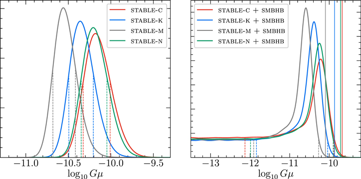
Figure 9. Reconstructed 1D marginalized posterior distributions for the dimensionless cosmic-string tension parameter G μ in the four stable-string models without SMBHBs (stable-c, stable-k, stable-m, and stable-n) in the left panel and including SMBHBs (stable-c+smbhb, stable-k+smbhb, stable-m+smbhb, and stable-n+smbhb) in the right panel. The dashed vertical lines show the 68% Bayesian credible intervals, which we construct as described in the text, and the solid vertical lines mark the G μ values where the K ratio in Equation (10) reaches a value of 1/10. Figure 28 in Appendix C.4 shows an extended version of this plot that includes the SMBHB parameters ABHB and γBHB.
Download figure:
Standard image High-resolution imageIf we extend the stable-string models by including an SMBHB contribution to the GW signal, the posterior distributions feature not only a peak toward the upper end of the  range but also an extended plateau at small
  values. This plateau corresponds precisely to the plateau that we alluded to in the definition of the K ratio in Equation (10) and hence allows us to derive the following upper limits on the cosmic-string tension in the stable-c+smbhb, stable-k+smbhb, stable-m+smbhb, and stable-n+smbhb models, respectively:
  , −9.87, −10.10, and −9.71. We recall that, for cosmic-string tensions exceeding these values, the likelihood of the strings-plus-SMBHBs model drops below 1/10 of the likelihood of the smbhb benchmark model. In this region of parameter space, adding GWs from stable strings to the signal does more harm than good and is strongly disfavored by the data. For comparison, we also quote the upper limits of the 95% Bayesian credible intervals for G
μ, specifically of the 95% highest posterior density intervals (HPDIs). For each model, the HPDI is the narrowest possible range that includes 95% of the posterior probability. By construction, the boundaries of an HPDI are at points with the same posterior probability density, and each parameter value inside the HPDI has higher posterior probability density than any parameter value outside the HPDI.
86
We find
, −9.87, −10.10, and −9.71. We recall that, for cosmic-string tensions exceeding these values, the likelihood of the strings-plus-SMBHBs model drops below 1/10 of the likelihood of the smbhb benchmark model. In this region of parameter space, adding GWs from stable strings to the signal does more harm than good and is strongly disfavored by the data. For comparison, we also quote the upper limits of the 95% Bayesian credible intervals for G
μ, specifically of the 95% highest posterior density intervals (HPDIs). For each model, the HPDI is the narrowest possible range that includes 95% of the posterior probability. By construction, the boundaries of an HPDI are at points with the same posterior probability density, and each parameter value inside the HPDI has higher posterior probability density than any parameter value outside the HPDI.
86
We find  , −10.04, −10.26, and −9.90 for stable-c+smbhb, stable-k+smbhb, stable-m+smbhb, and stable-n+smbhb, respectively.
Next, we turn to metastable strings, which, as can be read off from Figure 2, provide a better fit to the data. In the absence of an SMBHB contribution to the GW signal, the Bayes factors for the meta-l and meta-ls models are  and
and  , respectively. Adding an SMBHB contribution to the GW signal, the Bayes factors for the meta-l and meta-ls models are instead
  and
and  , respectively. Again, the fit does not become better, but the larger prior volume results in a decrease of the Bayes factors.
The reconstructed 1D and 2D posterior distributions for the two metastable-string models are shown in the corner plots in Figure 10. From these plots, we read off that the NG15 data prefer values of the decay parameter  of around
  in combination with a large cosmic-string tension,
  . Here
  causes a suppression of the GW signal in the nanohertz band compared to stable strings because of the exponential factor in Equation (50). This suppression results in a decreased signal strength and a larger spectral tilt. The decrease in signal strength can, however, be compensated by a large cosmic-string tension, such that the final spectrum still has the right amplitude but is now more blue-tilted than in the stable-string case. This interplay of the different factors affecting the GW spectrum from metastable strings effectively leads to a better fit.
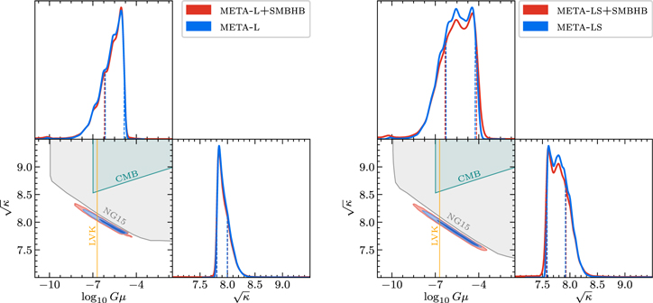
Figure 10. Same as in Figure 5 but for the metastable-string models meta-l (GW emissions from loops only) in the left panel and meta-ls (GW emission from loops and segments) in the right panel. The gray shaded regions are strongly disfavored by the NG15 data, as they result in a K ratio of less than 1/10 (see Equation (10)); the teal shaded regions are ruled out by the CMB bound on cosmic strings (Ade et al. 2016; Charnock et al. 2016; Lizarraga et al. 2016), and the regions to the right of the yellow contour lines violate the LVK bound in Equation (24). Figure 29 in Appendix C.4 shows extended versions of the two plots that include the SMBHB parameters ABHB and γBHB.
Download figure:
Standard image High-resolution imageLet us comment on a few characteristic features of the posterior distributions shown in Figure 10. First, we find that the  posterior in the meta-ls model extends to slightly larger values than in the meta-l model, which demonstrates the effect of the additional contribution to the GW signal from string segments. In fact, in the region of highest posterior density, the segment contribution dominates over the loop contribution in the meta-ls model. Second, we point out that the 1D marginalized posterior distributions for
  exhibit small local maxima at
  , which correspond to the stable-string limit within the metastable-string models. This limit is realized for large values of the decay parameter,
  , which pushes the effect of the network decay to frequencies below the PTA band. Next, we observe that for meta-l the
  posterior experiences a sharp drop-off at
  , whereas for meta-ls there is a small dip in the
  posterior at
  . Both features can be traced back to the Heaviside theta function in Equation (46), which ensures that no more new loops are formed during the decay regime of the network. Because of this Heaviside theta function, the loop contribution to the GW spectrum moves to frequencies above the PTA band if we raise
  above
above  . In this sense, the drop-off and the dip in the
  posteriors should be regarded as being due to our simplified theoretical modeling of the GW spectrum. More work is necessary to improve on the description in terms of a simple Heaviside theta function and obtain a better understanding of the evolution of the decaying network. We expect that a more accurate description of the transition from the scaling to the decay regime would result in smoother
  posteriors. Finally, we note that some of the fluctuations in the posteriors in Figure 10 can be attributed to the fact that, in the case of the metastable-string models, we have to work with tabulated data for the GW spectrum, based on the numerical evaluation of Equation (40).
We also use the corner plots in Figure 10 to highlight the relevant bounds on the parameter space spanned by  and
and  . The gray shaded areas notably indicate the K-ratio bound, which marks the parameter regions that are ruled out by the NANOGrav data. In these regions, the GW signal from metastable strings exceeds the observed signal and hence is unacceptably large. We find that the NANOGrav bound is stronger than the well-known CMB bound, which demands that a cosmic-string network that has not yet decayed by the time of recombination must not have a cosmic-string tension larger than
  (Ade et al. 2016; Charnock et al. 2016; Lizarraga et al. 2016). In order to derive the CMB bound, we estimate that a decaying network completely disappears because of GW emission at times around
  , which is the time when the second term in the exponent in Equation (50) becomes large. The teal shaded areas in Figure 10 indicate where the conditions
  and te
> trec ≃ 370,000 yr are satisfied simultaneously. Last but not least, the yellow solid lines represent the LVK bound in Equation (24), which translates to the upper limit G
μ ≲ 2 × 10⁻⁷.
87
and te
> trec ≃ 370,000 yr are satisfied simultaneously. Last but not least, the yellow solid lines represent the LVK bound in Equation (24), which translates to the upper limit G
μ ≲ 2 × 10⁻⁷.
87
The LVK bound on the amplitude of the stochastic GWB appears to be in tension with most of the parameter space preferred by the NANOGrav data. In particular, the 68% credible regions in the  –
– parameter plane are mostly ruled out by this bound. However, we stress that the LVK bound in Figure 10 relies on an extrapolation of the GW signal across 10 orders of magnitude in frequency, from PTA frequencies, f ∼ few × 10−9 nHz, to LVK frequencies, f ∼ few × 10 Hz. In order to perform this extrapolation, we have to assume a cosmological expansion history across 10 orders of magnitude in temperature, even though not much is known about the equation of state of the universe prior to BBN. Any deviation from the expansion history of standard big bang cosmology can therefore affect the extrapolation of the GW spectrum to higher frequencies and potentially render the LVK bound harmless. A simple example is an early stage of matter domination (Allahverdi et al. 2021), which would suppress the GW signal from metastable strings at high frequencies and thus allow for the possibility of cosmic-string tensions as large as those in Figure 10. On the other hand, if we trust the extrapolation to higher frequencies, we conclude that some parts of the 95% credible regions in Figure 10 are in fact not ruled out. In this case, metastable strings with
  and
and  are still able to provide a good fit of the data, which represents a particularly interesting scenario for two reasons: a value of
  would point to a GUT origin of the string network, and ground-based interferometers would be poised to detect the stochastic GWB signal from such a network in the near future.
Finally, we discuss our results for cosmic superstrings, for which we obtain the largest Bayes factors among all cosmic-string models considered in this work:  for GWs from superstrings alone and
  for an SMBHB contribution added to the superstring GW signal, both compared to the smbhb model.
Superstrings result in a good fit of the data because, unlike ordinary stable strings, they permit a GW signal that is neither too weak nor too flat. To see this, note that small cosmic-string tensions,  , yield a blue-tilted h2ΩGW spectrum at nanohertz frequencies (see our discussion above). In the case of ordinary strings, the amplitude of this spectrum would be too weak; however, for superstrings the suppression of the GW signal at
  can be compensated by the 1/P enhancement factor in Equation (52). By choosing P appropriately, the amplitude of the GW signal can then be raised until a good fit of the data is reached. This interplay between the two parameters of the super model can also be observed in Figure 11. The 2D posterior distribution for
  and P in this corner plot displays a strong covariance in line with our heuristic understanding.

Figure 11. Same as in Figure 10, but for the super model. Figure 30 in Appendix C.4 shows an extended version of this plot that includes the SMBHB parameters ABHB and γBHB.
Download figure:
Standard image High-resolution imageThe highest posterior density is achieved at small intercommutation probabilities and cosmic-string tensions,  and
and  , where
  corresponds in fact to the edge of the prior range for P. This parameter region is in tension with the LVK bound in Equation (24) (see the yellow solid line in Figure 11) but may be viable assuming a nonstandard expansion history at high temperatures. Similarly to what is found in Figure 10, we highlight the region ruled out by the NG15 data because it leads to a K ratio of less than 1/10. As expected, this region is located to the lower right of the 68% and 95% credible regions, where small
  values cause the amplitude of the GW spectrum to exceed the measured strength of the signal. The tension of cosmic superstrings can also be constrained by CMB observations (Charnock et al. 2016). Existing upper limits are, however, located at larger G
μ values and thus not relevant for our results in Figure 11.
values cause the amplitude of the GW spectrum to exceed the measured strength of the signal. The tension of cosmic superstrings can also be constrained by CMB observations (Charnock et al. 2016). Existing upper limits are, however, located at larger G
μ values and thus not relevant for our results in Figure 11.
In conclusion, we stress again that the GW spectrum from cosmic superstrings is not well understood at present, and more work is needed to arrive at a reliable prediction. Such an effort will be important to confirm that GWs from cosmic superstrings do indeed represent a realistic and viable interpretation of the PTA signal.
5.5. Domain Walls
5.5.1. Model Description
Domain walls are 2D topological defects that form when a cosmological phase transition results in the spontaneous breaking of a discrete symmetry, filling the universe with patches in different degenerate vacua (Kibble 1976). In the absence of significant interactions with relativistic particles, domain wall networks are expected to reach a scaling regime in which each Hubble volume, H−3, contains  domain walls (see, e.g., Press et al. 1989; Hindmarsh 1996, 2003; Garagounis & Hindmarsh 2003). In this regime, the energy density stored in domain walls is given by

where  is nearly constant and σ is the domain wall tension, which gives the domain walls their surface energy density. During the scaling regime, the energy density stored in domain walls dilutes more slowly than that of relativistic radiation and nonrelativistic matter. Indeed, the total energy density of the background always scales like ρc
∝ H2, which means that ΩDW = ρDW/ρc
grows like the Hubble radius when the domain wall network is in the scaling regime, ΩDW ∝ H−1. Therefore, domain walls eventually overclose the universe and alter the cosmological evolution in a way that is incompatible with CMB observations (Zeldovich et al. 1974). A possible solution to this problem is to have domain walls decay at some temperature T* by assuming, e.g., that the global symmetry responsible for domain wall formation is explicitly broken. Indeed, an explicit breaking of the symmetry introduces a bias among the possible low-energy vacua, thus lifting their degeneracy, which eventually leads to the collapse of the domain wall network (Vilenkin 1981b; Gelmini et al. 1989; Larsson et al. 1997).
is nearly constant and σ is the domain wall tension, which gives the domain walls their surface energy density. During the scaling regime, the energy density stored in domain walls dilutes more slowly than that of relativistic radiation and nonrelativistic matter. Indeed, the total energy density of the background always scales like ρc
∝ H2, which means that ΩDW = ρDW/ρc
grows like the Hubble radius when the domain wall network is in the scaling regime, ΩDW ∝ H−1. Therefore, domain walls eventually overclose the universe and alter the cosmological evolution in a way that is incompatible with CMB observations (Zeldovich et al. 1974). A possible solution to this problem is to have domain walls decay at some temperature T* by assuming, e.g., that the global symmetry responsible for domain wall formation is explicitly broken. Indeed, an explicit breaking of the symmetry introduces a bias among the possible low-energy vacua, thus lifting their degeneracy, which eventually leads to the collapse of the domain wall network (Vilenkin 1981b; Gelmini et al. 1989; Larsson et al. 1997).
During the scaling regime, domain walls continuously change their configuration and shrink in order to maintain the scaling relation in Equation (53). While these processes take place, a fraction of the domain wall energy is released in the form of GWs, which produce a GWB with a present-day relic abundance given by (Vilenkin 1981b; Preskill et al. 1991; Gleiser & Roberts 1998; Chang et al. 1999; Hiramatsu et al. 2010; Kawasaki & Saikawa 2011)

where  is the dilution factor defined in Equation (35),
  is an efficiency coefficient derived from numerical simulations (Hiramatsu et al. 2014), and α* is the fraction of the total energy density stored in domain walls at T*,

The GWB is dominated by the emission taking place just before the decay of the domain wall network. As the GWs are predominantly sourced by horizon-scale structures in the network, the typical frequency of the GWs emitted around this time is H*, i.e., the Hubble scale at T*. Therefore, after redshifting until today, the GWB is expected to exhibit a peak frequency
with both g* and g*,s
evaluated at T*. For the spectral shape,  , we use a parameterization similar to the one used for the phase transition spectrum in Section 5.3:
88
, we use a parameterization similar to the one used for the phase transition spectrum in Section 5.3:
88

Causality fixes a = 3, while numerical simulations (Hiramatsu et al. 2014) suggest b ≃ c ≃ 1. In our analysis, we therefore fix the low-frequency slope of the domain wall signal to the value predicted by causality, and, following Ferreira et al. (2022), we allow b and c to float within the uniform prior ranges b ∈ [0.5, 1] and c ∈ [0.3, 3].
In our analysis we consider two possible decay channels for the domain wall network: dark radiation (dw-dr) and SM particles (dw-sm). In the dw-dr model, instead of using α*, we parameterize the strength of the domain wall signal in terms of the dark radiation produced in the decay, ρDR. This quantity is usually expressed in terms of the effective number of extra neutrino species, ΔNeff, which we defined in Section 5.1 and which is bounded from above by BBN and CMB observations,  (Pisanti et al. 2021; Yeh et al. 2021). In our MCMC analysis of the dw-dr model, we follow Ferreira et al. (2022) and use
  as the upper bound on our prior for the parameter ΔNeff. Assuming that all the domain wall energy is converted to dark radiation at T*, ΔNeff is related to α* by
where, as before, both g* and g*,s are evaluated at T*.
In the dw-sm model, BBN restricts the possible values of the decay temperature to T* ≳ 2.7 MeV (Jedamzik 2006; Bai & Korwar 2022) for any detectable value of α*. Following Ferreira et al. (2022), we also impose α* < 0.3 to avoid any possible deviation from radiation domination and to evade bounds from ΔNeff.
5.5.2. Results and Discussion
The reconstructed posterior distributions for the parameters T* and α* (T* and ΔNeff) of the dw-sm (dw-dr) model are reported in Figure 12, for both the case where the domain walls are assumed to be the only source of GWs (blue contours) and the scenario where we consider the superposition of the domain wall and SMBHB signals (red contours). Full corner plots including the posterior distributions of the spectral shape parameters b and c are reported in Figure 31 in Appendix C.5.
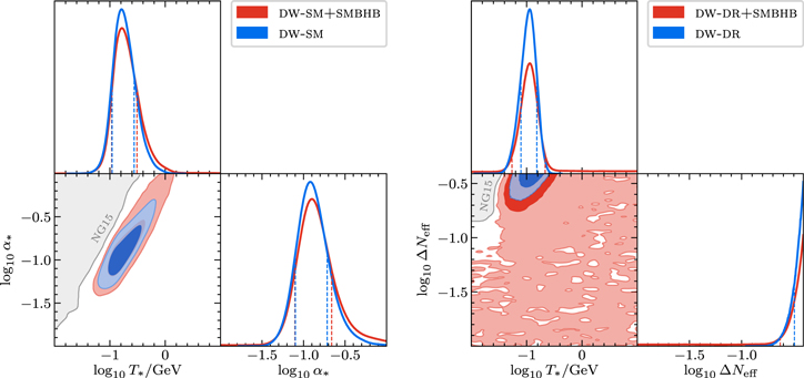
Figure 12. Same as in Figure 5, but for domain walls decaying to SM particles (left panel) and a dark sector (right panel). Figure 31 in Appendix C.5 shows extended versions of the two plots that include the spectral shape parameters b, c and the SMBHB parameters ABHB and γBHB.
Download figure:
Standard image High-resolution imageFor both the dw-sm and dw-dr models, with and without the inclusion of the SMBHB signal, we find that the GWB produced by domain walls peaks around 10−8 Hz such that most of the low frequency bins are fit by the low-frequency tail of the spectrum (see Figures 3 and 19). Specifically, for the dw-sm (dw-dr) model, we find that T* ∈ [110, 275] ([79, 153]) MeV at the 68% credible level and T* ∈ [76, 505] ([54, 198]) MeV at the 95% credible level. When including the SMBHB contribution to the GWB, we find T* ∈ [108, 309] ([54, 216]) MeV at the 68% credible level and T* ∈ [67, 843] (no bound on T*) MeV at the 95% credible level for the dw-sm (dw-dr) model. We notice that, with and without the inclusion of SMBHBs, the recovered transition temperature for the dw-sm model is high enough to evade BBN constraints.
For the dw-dr model, the posterior distribution for ΔNeff is peaked near the upper prior boundary, signaling that larger values fit the observed signal better. Specifically, we find ΔNeff ≳ 0.32 at the 68% credible level and ΔNeff ≳ 0.25 at the 95% credible level. Including the contribution from SMBHBs allows the distribution for ΔNeff to extend to lower values, and we find ΔNeff ≳ 0.23 at the 68% credible level and no bound at the 95% credible level. We thus conclude that the dw-dr model prefers large ΔNeff values in the vicinity of existing bounds. This means that the most promising parameter regions, i.e., regions that are not yet ruled by ΔNeff but still manage to fit the NANOGrav signal, point to ΔNeff values within the reach of upcoming experiments, including CMB-S4 (Abazajian et al. 2022), which promises to be sensitive to ΔNeff values as small as ΔNeff ≃ 0.06 at the 95% confidence level.
For the dw-sm model, we find α* ∈ [0.080, 0.19] at the 68% credible level and α* ∈ [0.053, 0.35] at the 95% credible level. With the inclusion of the SMBHB contribution, smaller values of α* become allowed, and we find α* ∈ [0.079, 0.22] at the 68% credible level and α* ∈ [0.047, 0.61] at the 95% credible level. We also notice a partial degeneracy between T* and α*, due to low frequency bins (which are the ones contributing the most to the evidence for a GWB) being fit by the low-frequency tail of the domain wall spectrum. Therefore, a shift to higher transition temperatures (and therefore to higher peak frequencies) can be partially reabsorbed with a shift to higher α* values.
For both dw models, we identify regions of the parameter space where the GW signal from domain walls is too strong to be compatible with NG15 data. These regions, shaded in gray in Figure 12, illustrate for the first time how PTA data can be used to constrain models of domain walls.
Finally, we state the Bayes factors for the model comparison between the domain wall models and the smbhb reference model. The Bayes factors for dw-sm and dw-dr versus smbhb are  and
and  , respectively, while the Bayes factors for dw-sm+smbhb and dw-dr+smbhb versus smbhb are
  and
and  , respectively. In both cases, the extra SMBHB contribution helps to improve the fit of the NG15 data. In the case of dw-dr, we moreover observe the same effect as for pt-sound in Section 5.3: adding the SMBHB contribution to the GWB signal results in a plateau region in the posterior distribution of the dw-dr model parameters that manifests itself as part of the 95% credible region in Figure 12.
6. Deterministic Signals from New Physics
In addition to the GWB signals discussed previously, there are several new-physics theories that can imprint a deterministic signal, described by a time series h , in pulsar timing data. In this section, we consider the deterministic signals induced by ULDM and DM substructures. After finding no statistically significant evidence for such signals in our data, we report upper limits on the allowed strength of these signals.
6.1. Ultralight Dark Matter
6.1.1. Model Description
While DM constitutes roughly 27% (Zyla et al. 2020) of the energy density of the universe, very little is known about its fundamental properties. Consequently, a wide range of DM models remain consistent with cosmological and astrophysical observations. The lightest possible DM particles are classified as ultralight, or fuzzy, DM. These particles must be bosonic; otherwise, they could not be packed into galaxies owing to Fermi degeneracy pressure (Tremaine & Gunn 1979; Di Paolo et al. 2018; Savchenko & Rudakovskyi 2019; Alvey et al. 2020; Davoudiasl et al. 2021). These ULDM models also generically suppress structure on small scales, allowing them to be potential solutions to the small-scale structure problems of the standard ΛCDM paradigm (Bullock & Boylan-Kolchin 2017). However, too much suppression on large scales would be in conflict with CMB measurements (Hlozek et al. 2015; Hložek et al. 2017, 2018), which sets a lower bound on the DM mass, 10−24 eV < mϕ . PTAs can probe these miniscule masses, since, as we describe below, the frequency of the ULDM signal, f, is generally proportional to the ULDM mass, 2π f ∼ mϕ . Therefore, the sensitivity window of NANOGrav is expected to be 10−23 eV ≲ mϕ ≲ 10−20 eV.
Other astrophysical constraints, such as measurements of the Lyα forest (Armengaud et al. 2017; Iršič et al. 2017; Kobayashi et al. 2017; Rogers & Peiris 2021), galactic subhalo mass functions (Schutz 2020; Banik et al. 2021; Nadler et al. 2021), and stellar kinematics (Dalal & Kravtsov 2022), can push this bound further up, ranging from 10−21 to 10−19 eV, and the nonobservation of superradiance at SMBHs (Arvanitaki et al. 2015; Stott 2020; Ünal et al. 2021) pushes the bound up to 10−21 ⋯ 10−17 eV. PTA searches for ULDM in the 10−23 eV ≲ mϕ ≲ 10−20 eV window can then be viewed as complementary to these astrophysical searches. Signals in PTAs do not depend on the same astrophysical uncertainties, e.g., modeling the nonlinear small-scale matter power spectrum with analytic or numeric methods (Zhang et al. 2018, 2019) or the evolution of specific density profiles. Moreover, the power of these methods quickly degrades when considering subcomponents of DM, or populations of DM that do not compose the whole DM density. The searches discussed here have a weaker dependence on the subcomponent fraction and are therefore still useful in the hunt for DM.
While there is a large phenomenology of ULDM signals that can be produced in PTAs, the timing residuals for the Ith pulsar, hI , are deterministic and can be written in the form

where i indexes the DM field polarization,
89
ω is the signal frequency, and we have split the signal into two terms: an "Earth term" with amplitude  and time-independent phase
  , and a "pulsar term" with amplitude
  and time-independent phase
  . The phases can be written as


where αi
(
x
) is dependent on the underlying ULDM field phase at point
x
, and the additional term in  is due to the light-travel time between Earth and the pulsar.
An important scale in understanding these signals is given by the correlation length of the ULDM field, ℓ c ,

where vϕ ∼ 10−3 is the ULDM velocity. If the correlation length is much larger than the distance between Earth and the pulsar, ℓc ≫ ∣ x E − x P,I ∣, both experience the same DM field. In this "correlated" limit of the signals, the amplitudes and phases can be taken to be position independent:

Generally, a correlated analysis can drastically reduce the number of free amplitude parameters in the MCMC. For example, if ULDM couples to all pulsars identically, then there is only one amplitude, AP , instead of one for each pulsar, to account for fluctuations in the ULDM field. However, since mϕ ∣ x E − x P,I ∣ ≫ 1, γP,I and γE must still be taken to be independent. In the uncorrelated limit, ℓc ≪ ∣ x E − x P,I ∣, the DM field is no longer correlated, and its amplitude fluctuations in different patches need to be accounted for.
In Table 1, we summarize the ULDM signals searched for in our analysis by providing the corresponding expression for the amplitudes and signal frequency appearing in Equation (59). In the following, we give a brief review of each of these signals and refer the reader to the original references for more details:
- 1.Metric fluctuations (Khmelnitsky & Rubakov 2014; Porayko & Postnov 2014; Porayko et al. 2018; Kato & Soda 2020; Nomura et al. 2020; Unal et al. 2022; Wu et al. 2022): Oscillations in the ULDM field generate fluctuations in the local stress-energy tensor, Tμ ν , which are independent of any direct couplings the ULDM may have with SM fields. These fluctuations in Tμ ν generate fluctuations in metric perturbations by Einstein's equations. These metric perturbations then affect the photon geodesic on its path from the pulsar and generate a timing residual with pulsar and Earth amplitudes given in Table 1. While the amplitudes shown in Table 1 are specific to scalar (spin-0) ULDM, vector (spin-1) ULDM also generates this purely gravitational signal. The vector DM scenario is more complicated (Nomura et al. 2020), as off-diagonal components of the metric fluctuations can generate nontrivial angular correlations between signals seen in different pulsars. In our analysis, we ignore these spatial correlations and set approximate bounds by treating the vector as three scalar components, such that the vector signal is three times larger than the scalar one (Nomura et al. 2020).
- 2.Doppler–U(1) forces (Graham et al. 2016; Xue et al. 2022): A background of ultralight vector DM can create dark "electric" fields, which can accelerate pulsars, or Earth, and Doppler-shift light arrival times. For example, if the DM is the gauge field of a local baryon symmetry, U(1)B , then it couples to the Earth and pulsar baryon current density. This coupling generates a force on both Earth and pulsars proportional to their baryon number, QB = NB × qB , where NB is the number of baryons and qB is the gauge charge. This scenario is straightforwardly generalized to other U(1) models, e.g., models where the difference between baryon and lepton numbers, B − L, is a local symmetry. These forces cause periodic displacements between Earth and pulsars and generate timing residuals with amplitudes given in Table 1. These forces also exist for scalar DM coupling to SM operators (e.g.,, where ϕ is the DM and n is the neutron field). However, in the scalar case, these forces originate from the field gradient ∇ϕ (Graham et al. 2016), which causes them to be velocity suppressed compared to the vector DM scenario.

Table 1. Summary of the Different Effects Induced by ULDM That Generate a Deterministic Signal of the Form Given in Equation (59)
| Effect |

|

| ω = 2π f | Spin (Sϕ ) |
|---|---|---|---|---|
| Metric fluctuations |

|
| 2mϕ | 0, 1 |
| Doppler–U(1) forces |
|
| mϕ | 1 |
| Pulsar spin fluctuations | 0 |

| mϕ | 0 |
| Reference clock shift |

| 0 | mϕ | 0 |
Note. "E" and "P" subscripts denote Earth and pulsar term contributions, respectively. Ai
is the signal amplitude for the ith DM polarization, ω is the signal frequency, and the "Spin" column refers to whether the effect occurs for scalar (spin-0) or vector (spin-1) ULDM candidates. ρϕ
is the local DM density, taken to be 0.4 GeV cm−3, mϕ
is the ULDM mass, g are gauge couplings, Q is the charge under the corresponding gauge group, y parameterizes the sensitivity to different fundamental constant fluctuations, d are defined in Equation (64), and  .
.  is a random variable representing the fluctuations in the ULDM field in different correlation patches; the correlated limit corresponds to
  . nI
is a vector pointing from Earth to the Ith pulsar, and
i
are the ULDM polarization vectors.
. nI
is a vector pointing from Earth to the Ith pulsar, and
i
are the ULDM polarization vectors.
Download table as: ASCIITypeset image
The next two signals we discuss are specific to scalar ULDM. All the linear couplings of a scalar ULDM field to the SM can be summarized in a single Lagrangian,
where Fμ
ν
and Gμ
ν
are the photon and gluon field strengths, respectively,  , β3 is the QCD beta function, γq
are the light quark anomalous dimensions, mf
are the fermion masses, and the d values are dimensionless couplings. These couplings induce periodic oscillations in the values of fundamental constants, i.e., particle masses and couplings, which can affect timing residuals in two ways:
, β3 is the QCD beta function, γq
are the light quark anomalous dimensions, mf
are the fermion masses, and the d values are dimensionless couplings. These couplings induce periodic oscillations in the values of fundamental constants, i.e., particle masses and couplings, which can affect timing residuals in two ways:
- 1.Pulsar spin fluctuations (Kaplan et al. 2022): Particle mass fluctuations change the moment of inertia of the pulsar, which, by conservation of angular momentum, leads to pulsar spin fluctuations. The amplitude of the signal is given in Table 1. The y parameters are pulsar specific and denote the pulsar sensitivity to a specific coupling, e.g., ye parameterizes the pulsar sensitivity to changes in the electron mass. parameterizes the pulsar sensitivity to the mass-weighted combination of quark mass couplings, . To be explicit, following Kaplan et al. (2022), we employ in our analysisfor each pulsar, which assumes the simplest possible model for the pulsars' moment of inertia.
- 2.Reference clock shifts (Graham et al. 2016; Kaplan et al. 2022): PTA timing residuals are measured with respect to a collection of mostly cesium (McCarthy 2009) atomic clocks. Therefore, changes to these atomic clock frequencies can appear in PTA data as apparent shifts in timing residuals. These shifts are perfectly correlated among pulsars and have the amplitude reported in Table 1. Similar to the pulsar spin fluctuation signal, the y parameters denote the atomic clock sensitivity to specific couplings. To be explicit, following Kaplan et al. (2022), we take these parameters to beassuming cesium clocks to be used as a reference.


6.1.2. Results and Discussion
We search for ULDM signals by performing a variety of Bayesian fit analyses on the NG15 data set. The priors for the ULDM model parameters are summarized in Table 3, while the priors for the intrinsic red-noise parameters are reported in Table 2. Since in this analysis we want to remain agnostic about the origin of the GWB, we model the GWB as a power law and allow the values of the amplitude and spectral index to float within the following prior ranges: ![${\mathrm{log}}_{10}{A}_{\mathrm{GWB}}\,\in [-18,-11]$](https://content.cld.iop.org/journals/2041-8205/951/1/L11/revision5/apjlacdc91ieqn258.gif) and γGWB ∈ [0, 7].
and γGWB ∈ [0, 7].
Over most of the ULDM mass range, 10−24 eV ≲ mϕ
≲ 10−20 eV, we find no significant evidence for any of the ULDM signals described in the previous section (with  in favor of models including a ULDM signal on top of the GWB). However, for ULDM models that give rise to an "Earth term" signal, we find mild evidence for an ULDM signal with frequency f ≃ 4 nHz. Specifically, restricting the prior range to f ∈ [3.05, 6.09] nHz, we find a Bayes factor of
  (
( ) in favor of the model including the ULDM signal in the correlated (uncorrelated) regime. This result is expected given the excess of monopolar-correlated power observed in the second frequency bin of the common red-noise process (see the discussion in NG15gwb for more details). Unfortunately, an ULDM interpretation of this monopolar signal is difficult, since the corresponding ULDM masses, mϕ
∼ 2 × 10⁻²³ eV, needed to explain this excess are in tension with other astrophysical bounds: Lyα forest (Armengaud et al. 2017; Iršič et al. 2017; Kobayashi et al. 2017; Rogers & Peiris 2021), galactic subhalo mass functions (Schutz 2020; Banik et al. 2021; Nadler et al. 2021), and stellar kinematics (Dalal & Kravtsov 2022).
) in favor of the model including the ULDM signal in the correlated (uncorrelated) regime. This result is expected given the excess of monopolar-correlated power observed in the second frequency bin of the common red-noise process (see the discussion in NG15gwb for more details). Unfortunately, an ULDM interpretation of this monopolar signal is difficult, since the corresponding ULDM masses, mϕ
∼ 2 × 10⁻²³ eV, needed to explain this excess are in tension with other astrophysical bounds: Lyα forest (Armengaud et al. 2017; Iršič et al. 2017; Kobayashi et al. 2017; Rogers & Peiris 2021), galactic subhalo mass functions (Schutz 2020; Banik et al. 2021; Nadler et al. 2021), and stellar kinematics (Dalal & Kravtsov 2022).
Without convincing evidence for a signal, we compute constraints on the ULDM model parameters, shown in Figures 13–15. All constraints are the 95th percentile of the marginalized posterior distribution for the parameter on the vertical axis. The curves labeled "(un)correlated" correspond to the analysis done in the (un)correlated limit, discussed in the previous section.
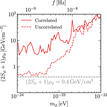
Figure 13. Constraints on the local ULDM density for the correlated (solid line) and uncorrelated (dashed line) signals at the 95% credible level (see the discussion in the text). The gray dashed line indicates the predicted DM abundance.
Download figure:
Standard image High-resolution image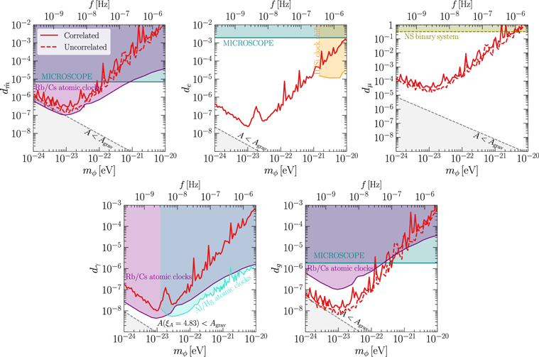
Figure 14. The red solid (dashed) lines show our constraints at the 95% credible level on the d parameters of the ULDM model, Equation (64), derived by searching for an (un)correlated signal. We assume that all reference clocks use the transition between the two hyperfine levels of the 133Cs ground state. Additionally, for each panel we assume that the d parameters not shown are set to zero. The lower gray shaded regions correspond to regions of parameter space where the signal amplitude is less than the purely gravitational signal. Current constraints "Rb/Cs atomic clocks" (purple) are from Hees et al. (2016), "Al/Hg atomic clocks" (turquoise) are from Boulder Atomic Clock Optical Network et al. (2005), "MICROSCOPE" (teal) are from Bergé et al. (2018), "H/Si clock shift" (orange) are from Boulder Atomic Clock Optical Network et al. (2005), and "NS binary system" are from Kumar Poddar et al. (2019) and Dror et al. (2020).
Download figure:
Standard image High-resolution image
Figure 15. The red solid (dashed) lines show our constraints at the 95% credible level for the two vector ULDM models considered in this analysis, for both the correlated (solid line) and uncorrelated (dashed line) regimes. The lower gray shaded regions correspond to regions of parameter space where the signal amplitude is smaller than the purely gravitational signal. The constraints from tests of the equivalence principle ("MICROSCOPE") are shown in teal (Bergé et al. 2018), and the constraints previously set by the PPTA Collaboration are reported in yellow (Xue et al. 2022).
Download figure:
Standard image High-resolution imageIn Figure 13, we show the constraints on the local ULDM energy density that can be derived assuming only gravitational coupling between the ULDM and SM fields. In Figure 13, we show the constraints on the local ULDM energy density that can be derived assuming only gravitational coupling between the ULDM and SM fields. The strongest bounds are obtained in the mass range mϕ
≲ 10−23 eV, where we nearly constrain ULDM to be a subcomponent of the total DM abundance. While we show constraints down to mϕ
= 10−24 eV, it is easy to extrapolate them to lower masses, where we expect them to remain flat down to m ∼ 10−26 eV, where 1/mϕ
becomes of the same order of the interpulsar separation and the ULDM signal is additionally suppressed (Khmelnitsky & Rubakov 2014; Unal et al. 2022). While future PTA analyses will be able to improve on these constraints, constraining ULDM with mϕ
≳ 10−23 eV to have a local abundance smaller than ρϕ
= 0.4 GeV cm−3 will be challenging, given that the constraints scale as  for mϕ
≳ 1/Tobs.
for mϕ
≳ 1/Tobs.
In Figure 14, we show the constraints for all the d parameters describing the scalar ULDM Lagrangian in Equation (64). Note that, for each panel, we assume that the parameter constrained is the only nonvanishing one. Overall, the limits are in rough agreement with the projections from Kaplan et al. (2022) and competitive with laboratory constraints (Boulder Atomic Clock Optical Network et al. 2005; Hees et al. 2016; Bergé et al. 2018; Kumar Poddar et al. 2019; Dror et al. 2020). The strongest constraints, relative to laboratory bounds, are for ULDM models coupled to the electron, de , and muon, dμ , mass terms. Indeed, relative shifts of the energy levels utilized in atomic clock experiments are insensitive to the de coupling, since atomic energy levels in different atoms scale identically with electron mass, leading to no relative energy level shifts (Van Tilburg et al. 2015; Kaplan et al. 2022). Such an insensitivity is not a problem for the PTA observable, though, since the pulsar phase evolution is not affected in the same way as the atomic energy levels. The lack of laboratory constraints on dμ is simply because there are not a large number of muons to study on Earth, whereas pulsars host a large number of them. As for the gravitational signal, we can extrapolate the constraints to lower masses, where we expect them to scale as d ∝ 1/mϕ down to mϕ ∼ 10−26 eV, where 1/mϕ becomes comparable to the interpulsar separation.
In Figure 15, we show constraints on the gauge coupling of models where the ULDM is the gauge boson of either U(1)B or U(1)B−L . Our constraints are roughly consistent with those published by the PPTA Collaboration (Porayko et al. 2018). This result is somewhat expected: while NANOGrav observes more pulsars, the average observation time is longer in PPTA, so roughly similar bounds are expected.
The constraints presented in Figures 14 and 15 assume that ULDM makes up the entire DM content of the universe. However, if ULDM is only a subcomponent of the total DM abundance, these constraints can be easily rescaled. Indeed, from Table 1, we see that the amplitudes for the direct coupling signals scale as  for the scalar case and
  for the vector case. Therefore, if ULDM is only a faction fϕ
of the total DM abundance, the constraints are weakened by a factor
for the vector case. Therefore, if ULDM is only a faction fϕ
of the total DM abundance, the constraints are weakened by a factor  .
.
Lastly, we comment on the prior choice for  . Previous studies (Porayko & Postnov 2014; Kato & Soda 2020) assumed that
  is not a random variable in the problem and placed constraints assuming that this parameter is simply 1. However, as pointed out by Centers et al. (2021), this assumption is not appropriate. Since the observation time of PTAs is much smaller than the coherence time of the DM,
  , only one instance of the field is being sampled within each correlation patch. The DM density in any correlation patch is then a random number, which follows a Rayleigh distribution with mean ρϕ
, and the priors should be chosen to reflect this. We also note that while Porayko et al. (2018) find the distribution of
, only one instance of the field is being sampled within each correlation patch. The DM density in any correlation patch is then a random number, which follows a Rayleigh distribution with mean ρϕ
, and the priors should be chosen to reflect this. We also note that while Porayko et al. (2018) find the distribution of  through numerical simulation, these results are consistent with the analytic predictions by Foster et al. (2018).
6.2. Dark Matter Substructures
6.2.1. Model Description
In the ΛCDM model, the structures we observe in the universe are seeded by primordial curvature fluctuations generated during inflation and then imprinted onto the DM density field. CMB observations indicate that these fluctuations have a nearly scale-invariant power spectrum on large scales (i.e., for comoving wavenumbers k ≃ Mpc−1). However, on smaller scales, various theories of DM leave unique fingerprints on primordial perturbations or their evolution, resulting in different predictions for the amount of subgalactic DM substructures. Consequently, measuring local DM substructures could be crucial in determining the correct model of DM.
PBHs are perhaps the simplest example of such small-scale DM substructures. They can be formed in inflationary theories that create large density fluctuations on small scales (like the ones described in Section 5.2). Several studies investigated the possibility of identifying a galactic PBH population by analyzing the Doppler and Shapiro signals they can leave in PTA data (Seto & Cooray 2007; Siegel et al. 2007; Dror et al. 2019; Ramani et al. 2020; Lee et al. 2021a, 2021b). In this analysis, we will closely follow the method outlined by Lee et al. (2021b) to constrain the local PBH abundance. 90
The Doppler signal results from the apparent shift in the pulsar spin frequency, generated by the acceleration induced by the gravitational pull of a passing PBH. According to the timescale of the transit event, τ, the signal can be further classified as dynamic (static) if τ is much smaller (larger) than the observation time, Tobs. In the static regime, the leading-order term of the Doppler signal that is not degenerate with the timing model is given by (Ramani et al. 2020; Lee et al. 2021a, 2021b)
where AD,sta is a dimensionless parameter that can be related to the kinematic parameters of the transiting event (see Appendix C.6 for more details). In the dynamic limit, and assuming that the signal is dominated by the closest transiting PBH, we get

where Θ is the Heaviside step function, AD,dyn is a dimensionless amplitude that can be related to kinematic parameters of the transiting event, and t0 is the time of closest approach (see Appendix C.6 for more details).
The Shapiro signal refers to shifts in the TOAs caused by metric perturbations along the photon geodesic produced by PBHs transiting along the observer's line of sight. In the static limit, and after subtracting away degeneracies with timing model parameters, the leading-order term of this signal can be parameterized as
where, as for the Doppler case, AS,sta is a dimensionless parameter that can be related to the kinematic parameters of the transiting event (see Appendix C.6 for more details). In the dynamic limit, there is no simple parameterization of the Shapiro signal; therefore, we do not search for this signal.
Assuming a monochromatic PBH population, our goal is to derive a posterior distribution for the PBH mass fraction, fPBH ≡ ΩPBH/ΩDM, as a function of the PBH mass, M: p(fPBH∣ δ t , M). We do this as follows:
- 1.For each given value of fPBH and M, we use the Monte Carlo code developed by Lee et al. (2021a) to generate a PBH population surrounding each of the pulsars in our array. From this distribution, we derive the amplitude of the static Doppler and Shapiro signals generated by the entire PBH population and the amplitude for the dynamic Doppler signal generated by the closest transiting PBH. Finally, we repeat this procedure for 2.5 × 10³ realizations to obtain the conditional probability distributions, where I indexes pulsars in the array and A refers to any of the PBH signal amplitudes introduced in Equations (67), (68), and (69). In Figure 16 we report some of the distributions derived in this way.
91
- 2.One at a time, we include the PBH signals given in Equations (67), (68), and (69) in the timing model, and we analyze our data to derive the posterior distributions for the various PBH signal amplitudes,. Since the PBH signal in different pulsars is assumed to be independent, these distributions can be factorized asSome of the are reported in Figure 16.
- 3.


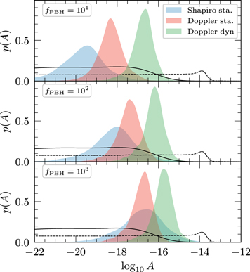
Figure 16. The black solid (dashed) lines show the posterior distributions  (
( ) for a representative pulsar (J1909−3744). The filled distributions show the conditional probability distributions
  for the same pulsar and different values of fPBH. In this plot, M = 10−6 (10−10) M⊙ for the Doppler static (dynamic) signal and M = 10 M⊙ for the Shapiro static signal.
Download figure:
Standard image High-resolution imageDM substructures can also possess macroscopic charges and interact with baryonic matter via long-range Yukawa interactions. These interactions can be modeled by a potential of the form

where M and MP
are the masses of the DM and pulsar, respectively, λ is the range of the interaction, and  is the effective DM−baryon coupling, normalized against the gravitational coupling (also known as the Yukawa parameter). Here the DM can be either a particle or a macroscopic object such as a nugget of asymmetric DM (Detmold et al. 2014; Wise & Zhang 2014; Hardy et al. 2015; Krnjaic & Sigurdson 2015; Gresham et al. 2017, 2018). These Yukawa interactions can arise from an effective Lagrangian of the form
  , where X and n are the effective DM and neutron fields, respectively, and ϕ is a massive (but potentially light) scalar or vector field. The effective coupling is related to the coupling constants by
  , where mn
is the neutron mass. These interactions are constrained to be weaker than gravity for the mass range M ≲ 100 GeV by the CMB, Lyα forest (Xu et al. 2018), and direct detection experiments such as X-ray Quantum Calorimeter (XQC; Mahdawi & Farrar 2018) and Cryogenic Rare Event Search with Superconducting Thermometers (CRESST; Angloher et al. 2017) (for a review on these constraints see Xu & Farrar 2020). However, stronger-than-gravity fifth forces are allowed if M ≫ 100 GeV, even when X accounts for the entirety of the DM population.
, where mn
is the neutron mass. These interactions are constrained to be weaker than gravity for the mass range M ≲ 100 GeV by the CMB, Lyα forest (Xu et al. 2018), and direct detection experiments such as X-ray Quantum Calorimeter (XQC; Mahdawi & Farrar 2018) and Cryogenic Rare Event Search with Superconducting Thermometers (CRESST; Angloher et al. 2017) (for a review on these constraints see Xu & Farrar 2020). However, stronger-than-gravity fifth forces are allowed if M ≫ 100 GeV, even when X accounts for the entirety of the DM population.
If present, these Yukawa interactions will contribute to the pulsar's acceleration induced by a transiting DM substructure and contribute to the Doppler signal discussed before (the expression for the Yukawa contribution to the Doppler signal can be found in Appendix C.6). Therefore, as shown by Gresham et al. (2023), following a procedure similar to the one used to constrain the abundance of PBHs, we can constrain the value of the Yukawa parameter,  . Specifically, for each given value of
  and M, we use the Monte Carlo code developed by Lee et al. (2021a) to generate a population of DM substructure surrounding each of the pulsars in our array. From this distribution, we derive the amplitude of the static Doppler signal generated by the closest transiting substructure by considering the acceleration induced by both the gravitational and Yukawa interaction. By repeating this procedure for multiple populations of DM substructure, we derive the distribution
  . By plugging this quantity into an expression similar to the one given in Equation (71), we can derive
  and use this quantity to constrain
  .
.
6.2.2. Results and Discussion
We start by searching for PBH signals on top of a GWB that we model as a power law with amplitude and spectral index allowed to float within the following prior ranges: ![${\mathrm{log}}_{10}{A}_{\mathrm{GWB}}\in [-11,-18]$](https://content.cld.iop.org/journals/2041-8205/951/1/L11/revision5/apjlacdc91ieqn287.gif) and γGWB ∈ [0, 7]. We find no statistically significant evidence for any of the PBH signals described in the previous section. Therefore, we proceed to set constraints on the local PBH abundance. The prior distributions used for the PBH signal parameters are reported in Table 3.
and γGWB ∈ [0, 7]. We find no statistically significant evidence for any of the PBH signals described in the previous section. Therefore, we proceed to set constraints on the local PBH abundance. The prior distributions used for the PBH signal parameters are reported in Table 3.
The 95% upper limits on fPBH derived from the static Doppler and Shapiro signals are reported in Figure 17. The dynamic Doppler signal is too weak to produce any detectable signal for any of the fPBH values considered. These are the first constraints on fPBH derived using real PTA data. As expected, our constraints are much weaker compared to the projections that were derived by Lee et al. (2021b) using mock data and including only white noise. Indeed, as already discussed by Lee et al. (2021b), the presence of a common red-noise process significantly reduces the sensitivity to PBH signals.

Figure 17. Constraints at the 95% credible level on the local PBH abundance derived from the search for static Doppler (red shaded region) and static Shapiro signals (blue shaded region). The solid lines interpolate between the PBH masses simulated in this work, while the red dashed line shows an extrapolation of the contraints to higher masses.
Download figure:
Standard image High-resolution imageFinally, in Figure 18 we show the constraints on  set by NG15 data. These constraints are compared with several other constraints that can be placed on
  . Specifically, in teal we show weak equivalence principle (WEP) constraints (Wagner et al. 2012; Shao et al. 2018; Sun et al. 2019; properly rescaled to take into account the finite range of the interaction, Gresham et al. 2023) derived by considering differential acceleration of baryonic test bodies toward the galactic center. In blue we report constraints from neutron star (NS) heating (assuming additional short-range DM−baryon interaction) induced by DM capture (Gresham et al. 2023), derived from the coldest known NS to date—PSR J2144−3933 (Guillot et al. 2019). In gray we report the indirect constraints that can be derived by combining the fifth-force constraints on baryon−baryon interactions (Bergé et al. 2018; Fayet 2019) and Bullet Cluster constraints on DM−DM interactions (Spergel & Steinhardt 2000; Kahlhoefer et al. 2014; see also Coskuner et al. 2019; Gresham et al. 2023). We find that the NG15 constraints are competitive with WEP and NS kinetic heating, especially in the M ≳ 10−12
M⊙ regime. However, the combined constraint from the Bullet Cluster and MICROSCOPE dominates over all other constraints in the entire mass range of interest. We note, however, that the combined constraint is an indirect probe of the Yukawa parameter and depends on the specific form of the light mediator coupling to DM and baryons. Specifically, in deriving the combined constraints, we have assumed that the Yukawa DM−baryon interaction arises from a Lagrangian of the form
. Specifically, in teal we show weak equivalence principle (WEP) constraints (Wagner et al. 2012; Shao et al. 2018; Sun et al. 2019; properly rescaled to take into account the finite range of the interaction, Gresham et al. 2023) derived by considering differential acceleration of baryonic test bodies toward the galactic center. In blue we report constraints from neutron star (NS) heating (assuming additional short-range DM−baryon interaction) induced by DM capture (Gresham et al. 2023), derived from the coldest known NS to date—PSR J2144−3933 (Guillot et al. 2019). In gray we report the indirect constraints that can be derived by combining the fifth-force constraints on baryon−baryon interactions (Bergé et al. 2018; Fayet 2019) and Bullet Cluster constraints on DM−DM interactions (Spergel & Steinhardt 2000; Kahlhoefer et al. 2014; see also Coskuner et al. 2019; Gresham et al. 2023). We find that the NG15 constraints are competitive with WEP and NS kinetic heating, especially in the M ≳ 10−12
M⊙ regime. However, the combined constraint from the Bullet Cluster and MICROSCOPE dominates over all other constraints in the entire mass range of interest. We note, however, that the combined constraint is an indirect probe of the Yukawa parameter and depends on the specific form of the light mediator coupling to DM and baryons. Specifically, in deriving the combined constraints, we have assumed that the Yukawa DM−baryon interaction arises from a Lagrangian of the form  . In addition, if only a subcomponent of DM interacts through the long-range fifth force, then the Bullet Cluster constraint will quickly lift, while the other constraints only deteriorate linearly with the DM fraction.

Figure 18. The 95% credible level for the fifth-force strength  derived from the NG15 data (red lines) is compared with constraints from NS kinetic heating (blue lines), equivalence principle constraints (green lines), and Bullet Cluster + equivalence principle constraints (gray line). Solid (dashed) lines are deriving assuming λ = 1 pc (λ = 10−1 pc), while dashed–dotted (dotted) lines are derived assuming λ = 10−2 pc (λ = 10−3 pc).
Download figure:
Standard image High-resolution image7. Discussion
The analysis of the NANOGrav 15 yr data set has produced the first convincing evidence for a stochastic background of GWs in the nanohertz frequency range. The origin of this background is still unknown. In this work, we considered various cosmological sources and compared them to the commonly studied astrophysical signal produced by a population of inspiraling SMBHBs. Specifically, we considered the signals produced by nonminimal inflation scenarios, SIGWs, cosmological phase transitions, several cosmic-string models, and domain walls.
For each of these models, we identified regions of the parameter space that are compatible with the observed signal. We find that, with the exception of stable cosmic strings of field theory origin, all new-physics models considered in this analysis are capable of reproducing the GWB signal. Many models allow us in fact to fit the signal better than the SMBHB reference model, which is reflected in Bayes factors ranging from 10 to 100 (see Figure 2). When the new-physics signals are combined with the astrophysical one, we obtain comparable results. More precisely, in several models, the addition of the SMBHB signal leads to a slight decrease of the Bayes factor, which indicates that the SMBHB contribution does not help to improve the quality of the fit but merely increases the prior volume. In other models, on the other hand, such as pt-sound and dw-dr, adding the SMBHB signal on top of the new-physics signal can lead to a slight increase of the Bayes factor, indicating that the SMBHB signal can in fact play a dominant role in the total GW spectrum. For all four stable-string models, we find Bayes factors between 0.1 and 1. Cosmic superstrings, on the other hand, which are also stable but not of field theory origin, can explain the data at a level comparable to other new-physics sources.
Despite the fact that some of the Bayes factors derived in this paper might suggest that a purely astrophysical interpretation of the signal is disfavored by the data, we caution against this interpretation. The Bayes factors do not account for the full range of uncertainties in both the cosmological and astrophysical signals and are prior dependent. It is conceivable that, as our understanding of SMBHB signals and our noise models improve, the tension between observations and astrophysical predictions will decrease, potentially weakening the evidence in favor of cosmological signals.
Future data sets will improve the spectral characterization of the signal and improve our ability to discriminate cosmological sources from the SMBHB signal. Unfortunately, similarities in the spectral shape and theoretical uncertainties will make it challenging to definitively determine the origin of the background using power spectrum characterization alone. However, the observation of anisotropies could eventually resolve this debate, as the expected anisotropies generated by black hole binaries are significantly larger than those produced by most cosmological sources. Similarly, the detection of a continuous wave from a single binary would provide convincing evidence in favor of an astrophysical origin of the signal. Ultimately, measurements of the GWB spectral shape and angular power spectrum may be complemented by observations of its polarization content and possible deviations from Gaussian statistics, which can again help to discriminate between an astrophysical and a cosmological origin of the signal.
It is worth emphasizing that in all parts of our analysis we described cosmological signals using effective parameters, e.g., T*, α*, and H* R*, for the phase transition models. Moving forward, it will be crucial to identify microscopic models that can reproduce the values of these parameters that we found to best fit the GWB signal. That is, in order to shed more light on the various cosmological interpretations of the signal, we require a better understanding of how the NANOGrav signal could possibly result from the fundamental parameters of a particle physics Lagrangian that describes the generation of GWs in the early universe.
Along with searching for a cosmological GWB, we also analyze our data to search for deterministic signals generated by models of ULDM and DM substructures. We do not find significant evidence for either of these signals. Nonetheless, we are able to place constraints on the parameters space of these models. For a wide range of ULDM models, our constraints compete or outperform laboratory constraints in the 10−23 eV ≲ mϕ ≲ 10−20 eV mass window. The signal from DM substructures is harder to detect; as a consequence, we are able to set very weak constraints on the local abundance of these objects. Future data sets will improve our reach, but a better characterization of the GWB will be needed to probe realistic models of DM substructures.
The discovery of a GWB will lead to significant breakthroughs in our understanding of cosmology and particle physics. As future PTA data sets become available, we will establish the origin of the GWB. Regardless of whether the signal is of cosmological origin, we have shown how PTAs will undoubtedly contribute to exploring new physics, either as a discovery tool or as a new way to constrain the parameter space of BSM models.
Acknowledgments
A.Mi. proposed and initiated the project. A.Mi. and K.Sc. coordinated and led the search. The enterprise wrapper, PTArcade (Mitridate et al. 2023, in preparation), used in this analysis was mainly developed by A.Mi., with help from D.W., K.D.O., J.N., R.v.E., T.S., and T.T. R.v.E. and T.S. developed the statistical tools needed to derive the K-ratio bounds. L.Z.K. derived the distributions of power-law fit parameters for characteristic strain spectra from SMBHB simulations. A.Mi. prepared all figures except those in Section 6.1, which were prepared by T.T.; Figure 18, which was prepared by V.L.; and Figure 22, which was prepared by R.R.L.d.S. A.Mi. and K.Sc. wrote the paper with help from K.B., K.D.O., S.Ve., and T.T.
Contributions to specific analyses are as follows. K.Sc. led and discussed the results of the SIGW and IGW analyses, which were performed by D.W. and R.R.L.d.S. A.Af. and R.R.L.d.S. derived the constraints on the parameter space of the SIGW model. D.W. and R.R.L.d.S. derived the LVK and Neff bounds on the IGW model. A.Mi. led the PT analysis, which was performed by both A.Mi. and R.v.E.; A.Mi. and K.Sc. interpreted and discussed the results. The string analyses were led by K.D.O. and K.Sc., with K.D.O., K.Sc., and T.S. conducting the analyses; K.Sc. interpreted and discussed the results with help from K.D.O. and J.J.B.P. A.Mi. led the domain wall analysis, which was performed by both A.Mi. and D.W.; A.Mi. and K.Sc. interpreted and discussed the results. The ULDM analysis was coordinated by A.Mi., K.B., and T.T.; J.N. performed the analysis; and A.Mi., C.U., K.B., J.N., and T.T. interpreted and discussed the results. Finally, the substructure search was led by A.Mi. and T.T.; A.Mi., S.Ve., and V.L. performed the analysis; and A.Mi., S.Ve., V.L., and T.T. interpreted and discussed the results.
The NANOGrav Collaboration receives support from National Science Foundation (NSF) Physics Frontiers Center award Nos. 1430284 and 2020265, the Gordon and Betty Moore Foundation, NSF AccelNet award No. 2114721, an NSERC Discovery Grant, and CIFAR. The Arecibo Observatory is a facility of the NSF operated under cooperative agreement (AST-1744119) by the University of Central Florida (UCF) in alliance with Universidad Ana G. Méndez (UAGM) and Yang Enterprises (YEI), Inc. The Green Bank Observatory is a facility of the NSF operated under cooperative agreement by Associated Universities, Inc. The National Radio Astronomy Observatory is a facility of the NSF operated under cooperative agreement by Associated Universities, Inc. NANOGrav is part of the International Pulsar Timing Array (IPTA); we would like to thank our IPTA colleagues for their help with this paper.
Part of this work was conducted using the High Performance Computing Cluster PALMA II at the University of Münster (https://www.uni-muenster.de/IT/HPC). This work used the Maxwell computational resources operated at Deutsches Elektronen-Synchrotron DESY, Hamburg (Germany). This work was conducted in part using the HPC resources of the Texas Advanced Computing Center (TACC) at the University of Texas at Austin. The Tufts University High Performance Computing Cluster (https://it.tufts.edu/high-performance-computing) was utilized for some of the research reported in this paper. This research used the computational resources provided by the University of Central Florida's Advanced Research Computing Center.
J.J.B.P. acknowledges the support by the PID2021-123703NB-C21 grant funded by MCIN/AEI /10.13039/501100011033/ and by ERDF; "A way of making Europe," the Basque Government grant (IT-1628-22); and the Basque Foundation for Science (IKERBASQUE). L.B. acknowledges support from the National Science Foundation under award AST-1909933 and from the Research Corporation for Science Advancement under Cottrell Scholar Award No. 27553. P.R.B. is supported by the Science and Technology Facilities Council, grant No. ST/W000946/1. S.B. gratefully acknowledges the support of a Sloan Fellowship and the support of NSF under award No. 1815664. M.C. and S.R.T. acknowledge support from NSF AST-2007993. M.C. and N.S.P. were supported by the Vanderbilt Initiative in Data Intensive Astrophysics (VIDA) Fellowship. Support for this work was provided by the NSF through the Grote Reber Fellowship Program administered by Associated Universities, Inc./National Radio Astronomy Observatory. Support for H.T.C. is provided by NASA through the NASA Hubble Fellowship Program grant No. HST-HF2-51453.001 awarded by the Space Telescope Science Institute, which is operated by the Association of Universities for Research in Astronomy, Inc., for NASA, under contract NAS5-26555. K.C. is supported by a UBC Four Year Fellowship (6456). M.E.D. acknowledges support from the Naval Research Laboratory by NASA under contract S-15633Y. T.D. and M.T.L. are supported by an NSF Astronomy and Astrophysics Grant (AAG), award No. 2009468. The work of R.v.E., K. Sc., and T.S. is supported by the Deutsche Forschungsgemeinschaft (DFG) through the Research Training Group, GRK 2149: Strong and Weak Interactions—from Hadrons to Dark Matter. E.C.F. is supported by NASA under award No. 80GSFC21M0002. G.E.F., S.C.S., and S.J.V. are supported by NSF award PHY-2011772. The Flatiron Institute is supported by the Simons Foundation. A.D.J. and M.V. acknowledge support from the Caltech and Jet Propulsion Laboratory President's and Director's Research and Development Fund. A.D.J. acknowledges support from the Sloan Foundation. The work of N.La. and X.S. is partly supported by the George and Hannah Bolinger Memorial Fund in the College of Science at Oregon State University. N.La. acknowledges the support from Larry W. Martin and Joyce B. O'Neill Endowed Fellowship in the College of Science at Oregon State University. Part of this research was carried out at the Jet Propulsion Laboratory, California Institute of Technology, under a contract with the National Aeronautics and Space Administration (80NM0018D0004). V.S.H.L. is supported by the DoE under contract DE-SC0011632. R.R.L.d.S. is supported by a research grant (29405) from VILLUM FONDEN. D.R.L. and M.A.M. are supported by NSF No. 1458952. M.A.M. is supported by NSF No. 2009425. C.M.F.M. was supported in part by the National Science Foundation under grant Nos. NSF PHY-1748958 and AST-2106552. A.Mi. is supported by the Deutsche Forschungsgemeinschaft under Germany's Excellence Strategy—EXC 2121 Quantum Universe—390833306. The Dunlap Institute is funded by an endowment established by the David Dunlap family and the University of Toronto. K.D.O. was supported in part by NSF grant Nos. 2111738 and 2207267. T.T.P. acknowledges support from the Extragalactic Astrophysics Research Group at Eötvös Loránd University, funded by the Eötvös Loránd Research Network (ELKH), which was used during the development of this research. S.M.R. and I.H.S. are CIFAR Fellows. Portions of this work performed at NRL were supported by ONR 6.1 basic research funding. J.D.R. also acknowledges support from start-up funds from Texas Tech University. J.S. is supported by an NSF Astronomy and Astrophysics Postdoctoral Fellowship under award AST-2202388 and acknowledges previous support by the NSF under award 1847938. S.R.T. acknowledges support from an NSF CAREER award No. 2146016. T.T.'s contribution to this work is supported by the Fermi Research Alliance, LLC, under contract No. DE-AC02-07CH11359 with the U.S. Department of Energy, Office of Science, Office of High Energy Physics. C.U. acknowledges support from BGU (Kreitman fellowship) and the Council for Higher Education and Israel Academy of Sciences and Humanities (Excellence fellowship). C.A.W. acknowledges support from CIERA, the Adler Planetarium, and the Brinson Foundation through a CIERA-Adler postdoctoral fellowship. O.Y. is supported by the National Science Foundation Graduate Research Fellowship under grant No. DGE-2139292. The work of K.Z. is also supported by a SimonsInvestigator award and the U.S. Department of Energy, Office of Science, Office of HighEnergy Physics, under Award No. DE-SC0011632.
Author Contributions
An alphabetical-order author list was used for this paper in recognition of the fact that a large, decade-timescale project such as NANOGrav is necessarily the result of the work of many people. All authors contributed to the activities of the NANOGrav Collaboration leading to the work presented here and reviewed the manuscript, text, and figures prior to the paper's submission. Additional specific contributions to this paper are as given in the acknowledgments.
Appendix A: Parameter Ranges and Limits
In this appendix, we specify the prior assumptions for all model parameters used in our analyses and report characteristic values for these parameters that we extract from the corresponding reconstructed 1D marginalized posterior distributions. In Table 2, we list our prior assumptions for the pulsar-intrinsic red-noise parameters Ared and γred (Aa
and γa
in Equation (4)), as well as for the SMBHB parameters ABHB and γBHB. In the latter case, we work with a bivariate normal distribution for  whose mean and covariance matrix are given by

which we obtain by fitting the  and γBHB distributions extracted from the SMBHB simulations in the GWOnly-Ext library in NG15smbh (see Section 4). In Table 3 we list our prior assumptions for the model parameters of all new-physics models considered in this work, and in Table 4 we summarize various key values extracted from the corresponding 1D marginalized posterior distributions. Specifically, we report the Bayes estimator, including its standard deviation; the maximum posterior estimator, including the 68% credible interval; and (when applicable) the upper bound based on the requirement that the K ratio in Equation (10) should not be smaller than 1/10.
Table 2. Prior Distributions for the Pulsar-intrinsic Red-noise Parameters and the Parameters of the Astrophysical SMBHB Signal
| Parameter | Description | Prior | Comments |
|---|---|---|---|
| Pulsar-intrinsic Red Noise | |||
| Ared | Red-noise power-law amplitude | Log-uniform [−20, − 11] | One parameter per pulsar |
| γred | Red-noise power-law spectral index | Uniform [0, 7] | One parameter per pulsar |
| Supermassive Black Hole Binaries (smbhb) | |||

| SMBHB signal amplitude and slope | Normal( μ BHB, σ BHB) | One parameter for PTA |
Note. The mean and covariance matrix of the Gaussian prior distribution for  are given in Equation (A1).
Download table as: ASCIITypeset image
Table 3. Prior Distributions for the Parameters of the New-physics Models Considered in This Work
| Parameter | Description | Prior | Comments |
|---|---|---|---|
| Inflationary Gravitational Waves (igw) | |||
| Trh [GeV] | Reheating temperature | Log-uniform [−3, 3] | One parameter per PTA |
| r | Tensor-to-scalar ratio | Log-uniform [−40, 0] | One parameter per PTA |
| nt | Tensor spectral index | Uniform [0, 6] | One parameter per PTA |
| Scalar-induced Gravitational Waves (sigw-delta) | |||
| A | Scalar amplitude | Log-uniform [−3, 1] | One parameter per PTA |
| f* [Hz] | Peak frequency | Log-uniform [−11, −5] | One parameter per PTA |
| Scalar-induced Gravitational Waves (sigw-Gauss) | |||
| A | Scalar amplitude | Log-uniform [−3, 1] | One parameter per PTA |
| f* [Hz] | Peak frequency | Log-uniform [−11, −5] | One parameter per PTA |
| Δ | Width | Uniform [0.1, 3] | One parameter per PTA |
| Scalar-induced Gravitational Waves (sigw-box) | |||
| A | Scalar amplitude | Log-uniform [−3, 1] | One parameter per PTA |
![${f}_{\min }\,[\mathrm{Hz}]$](https://content.cld.iop.org/journals/2041-8205/951/1/L11/revision5/apjlacdc91ieqn288.gif)
| Lower frequency | Log-uniform [−11, −5] | One parameter per PTA |
![${f}_{\max }\,[\mathrm{Hz}]$](https://content.cld.iop.org/journals/2041-8205/951/1/L11/revision5/apjlacdc91ieqn289.gif)
| Upper frequency | Log-uniform [−11, −5] | One parameter per PTA |
| Cosmological Phase Transition (pt) | |||
| T* [GeV] | Transition temperature | Log-uniform [−4, 4] | One parameter per PTA |
| α* | Transition strength | Log-uniform [−2, 1] | One parameter per PTA |
| H* R* | Bubble separation | Log-uniform [−3, 0] | One parameter per PTA |
| a | Low-frequency slope (pt-bubbles) | Uniform [1, 3] | One parameter per PTA |
| Low-frequency slope (pt-sound) | Uniform [3, 5] | One parameter per PTA | |
| b | High-frequency slope (pt-bubbles) | Uniform [1, 3] | One parameter per PTA |
| High-frequency slope (pt-sound) | Uniform [2, 4] | One parameter per PTA | |
| c | Spectral shape width (pt-bubbles) | Uniform [1, 3] | One parameter per PTA |
| Spectral shape width (pt-sound) | Uniform [3, 5] | One parameter per PTA | |
| Cosmic Strings (stable) | |||
| G μ | String tension | Log-uniform [−14, −6] | One parameter per PTA |
| Metastable Cosmic Strings (meta) | |||
| G μ | String tension | Log-uniform [−14, −1.5] | One parameter per PTA |

| Decay parameter | Uniform [7, 9.5] | One parameter per PTA |
| Cosmic Superstrings (super) | |||
| G μ | String tension | Log-uniform [−14, −6] | One parameter per PTA |
| P | Intercommutation probability | Log-uniform [−3, 0] | One parameter per PTA |
| Domain Walls (dw-sm) | |||
| T* [GeV] | Transition temperature | Log-uniform [−4, 4] | One parameter per PTA |
| α* | Energy fraction in domain walls | Log-uniform [−3, 0] | One parameter per PTA |
| b | High-frequency slope | Uniform [0.5, 1] | One parameter per PTA |
| c | Spectral shape width | Uniform [0.3, 3] | One parameter per PTA |
| Domain Walls (dw-ds) | |||
| T* [GeV] | Transition temperature | Log-uniform [−4, 4] | One parameter per PTA |
| ΔNeff | Amount of dark radiation | Log-uniform [−3, −0.41] | One parameter per PTA |
| b | High-frequency slope | Uniform [0.5, 1] | One parameter per PTA |
| c | Spectral shape width | Uniform [0.3, 3] | One parameter per PTA |
| Ultralight Dark Matter (ULDM) | |||
| Ai [s] | ULDM signal amplitude | Log-uniform [−9, −4] | One parameter per PTA |
| mϕ [eV] | ULDM mass | Log-uniform [−24, −19] | One parameter per PTA |

| Earth normalized signal amplitude | e−x | One parameter per PTA |

| Pulsar normalized signal amplitude | e−x | One parameter per pulsar* |
| γE | Earth signal phase | Uniform [0, 2π] | One parameter per PTA |
| γP | Pulsar signal phase | Uniform [0, 2π] | One parameter per pulsar |
| Primordial Black Holes (pbh-dynamic) | |||
| A | Signal amplitude | Log-uniform [−20, −12] | One parameter per PTA |
| T0/Tobs | Normalized time of closest approach | Uniform [0, 1] | One parameter per PTA |
| Primordial Black Holes (pbh-static) | |||
| A | Signal amplitude | Log-uniform [−21, −13] | One parameter per PTA |
Note. The asterisk indicates parameters that are present only in the uncorrelated ULDM analyses.
Download table as: ASCIITypeset image
Table 4. Bayesian Estimators, Maximum Posterior Values, and 68% Credible Intervals for the Parameters of the New-physics Models
| Parameter | Bayes Estimator | Maximum Posterior | 68% Credible Interval | K Bound | |||
|---|---|---|---|---|---|---|---|
| NP | NP+SMBHB | NP | NP+SMBHB | NP | NP+SMBHB | ||
| Inflationary Gravitational Waves (igw) | |||||||

| 0.02 ± 1.60 | −0.07 ± 1.61 | −0.53 | −0.60 |
![$\left[-1.51,2.53\right]$](https://content.cld.iop.org/journals/2041-8205/951/1/L11/revision5/apjlacdc91ieqn300.gif)
|
![$\left[-1.89,2.11\right]$](https://content.cld.iop.org/journals/2041-8205/951/1/L11/revision5/apjlacdc91ieqn301.gif)
| ⋯ |

| −14.06 ± 5.82 | −15.97 ± 7.27 | −10.14 | −10.59 |
![$\left[-22.16,-6.58\right]$](https://content.cld.iop.org/journals/2041-8205/951/1/L11/revision5/apjlacdc91ieqn303.gif)
|
![$\left[-23.03,-7.21\right]$](https://content.cld.iop.org/journals/2041-8205/951/1/L11/revision5/apjlacdc91ieqn304.gif)
| ⋯ |
| nt | 2.61 ± 0.85 | 2.68 ± 0.97 | 2.02 | 2.08 |
![$\left[1.53,3.92\right]$](https://content.cld.iop.org/journals/2041-8205/951/1/L11/revision5/apjlacdc91ieqn305.gif)
|
![$\left[1.56,4.03\right]$](https://content.cld.iop.org/journals/2041-8205/951/1/L11/revision5/apjlacdc91ieqn306.gif)
| 5.72 |

| ⋯ | −15.60 ± 0.56 | ⋯ | −15.64 | ⋯ |
![$\left[-16.20,-15.14\right]$](https://content.cld.iop.org/journals/2041-8205/951/1/L11/revision5/apjlacdc91ieqn308.gif)
| ⋯ |
| γBHB | ⋯ | 4.61 ± 0.37 | ⋯ | 4.64 | ⋯ |
![$\left[4.26,5.00\right]$](https://content.cld.iop.org/journals/2041-8205/951/1/L11/revision5/apjlacdc91ieqn309.gif)
| ⋯ |
| Scalar-induced Gravitational Waves (sigw-delta) | |||||||

| −0.69 ± 0.47 | −0.71 ± 0.49 | −0.14 | −0.17 |
![$\left[-1.00,-0.01\right]$](https://content.cld.iop.org/journals/2041-8205/951/1/L11/revision5/apjlacdc91ieqn311.gif)
|
![$\left[-1.03,-0.02\right]$](https://content.cld.iop.org/journals/2041-8205/951/1/L11/revision5/apjlacdc91ieqn312.gif)
| ⋯ |

| −5.90 ± 0.60 | −5.93 ± 0.67 | −5* | −5* |
![$\left[-6.17,-{5}^{* }\right]$](https://content.cld.iop.org/journals/2041-8205/951/1/L11/revision5/apjlacdc91ieqn314.gif)
|
![$\left[-6.19,-{5}^{* }\right]$](https://content.cld.iop.org/journals/2041-8205/951/1/L11/revision5/apjlacdc91ieqn315.gif)
| ⋯ |

| ⋯ | −15.77 ± 0.46 | ⋯ | −15.71 | ⋯ |
![$\left[-16.18,-15.29\right]$](https://content.cld.iop.org/journals/2041-8205/951/1/L11/revision5/apjlacdc91ieqn317.gif)
| ⋯ |
| γBHB | ⋯ | 4.65 ± 0.35 | ⋯ | 4.65 | ⋯ |
![$\left[4.31,4.99\right]$](https://content.cld.iop.org/journals/2041-8205/951/1/L11/revision5/apjlacdc91ieqn318.gif)
| ⋯ |
| Scalar-induced Gravitational Waves (sigw-Gauss) | |||||||

| −0.38 ± 0.58 | −0.36 ± 0.61 | −0.34 | −0.29 |
![$\left[-1.03,0.20\right]$](https://content.cld.iop.org/journals/2041-8205/951/1/L11/revision5/apjlacdc91ieqn320.gif)
|
![$\left[-1.04,0.24\right]$](https://content.cld.iop.org/journals/2041-8205/951/1/L11/revision5/apjlacdc91ieqn321.gif)
| ⋯ |

| −6.32 ± 0.71 | −6.30 ± 0.73 | −7.03 | −6.85 |
![$\left[-7.25,-5.65\right]$](https://content.cld.iop.org/journals/2041-8205/951/1/L11/revision5/apjlacdc91ieqn323.gif)
|
![$\left[-7.17,-5.57\right]$](https://content.cld.iop.org/journals/2041-8205/951/1/L11/revision5/apjlacdc91ieqn324.gif)
| ⋯ |
| Δ | 1.35 ± 0.70 | 1.30 ± 0.70 | 1.60 | 1.54 |
![$\left[0.51,2.07\right]$](https://content.cld.iop.org/journals/2041-8205/951/1/L11/revision5/apjlacdc91ieqn325.gif)
|
![$\left[0.37,1.92\right]$](https://content.cld.iop.org/journals/2041-8205/951/1/L11/revision5/apjlacdc91ieqn326.gif)
| ⋯ |

| ⋯ | −15.72 ± 0.46 | ⋯ | −15.65 | ⋯ |
![$\left[-16.14,-15.22\right]$](https://content.cld.iop.org/journals/2041-8205/951/1/L11/revision5/apjlacdc91ieqn328.gif)
| ⋯ |
| γBHB | ⋯ | 4.65 ± 0.34 | ⋯ | 4.65 | ⋯ |
![$\left[4.32,5.00\right]$](https://content.cld.iop.org/journals/2041-8205/951/1/L11/revision5/apjlacdc91ieqn329.gif)
| ⋯ |
| Scalar-induced Gravitational Waves (sigw-box) | |||||||

| −1.06 ± 0.52 | −1.02 ± 0.57 | −1.26 | −1.25 |
![$\left[-1.72,-0.82\right]$](https://content.cld.iop.org/journals/2041-8205/951/1/L11/revision5/apjlacdc91ieqn331.gif)
|
![$\left[-1.68,-0.74\right]$](https://content.cld.iop.org/journals/2041-8205/951/1/L11/revision5/apjlacdc91ieqn332.gif)
| ⋯ |

| −7.34 ± 0.48 | −7.29 ± 0.55 | −7.50 | −7.48 |
![$\left[-8.01,-6.97\right]$](https://content.cld.iop.org/journals/2041-8205/951/1/L11/revision5/apjlacdc91ieqn334.gif)
|
![$\left[-7.97,-6.84\right]$](https://content.cld.iop.org/journals/2041-8205/951/1/L11/revision5/apjlacdc91ieqn335.gif)
| ⋯ |

| −6.06 ± 0.65 | −6.12 ± 0.81 | −5.40 | −5.36 |
![$\left[-6.42,-{5}^{* }\right]$](https://content.cld.iop.org/journals/2041-8205/951/1/L11/revision5/apjlacdc91ieqn337.gif)
|
![$\left[-6.45,-{5}^{* }\right]$](https://content.cld.iop.org/journals/2041-8205/951/1/L11/revision5/apjlacdc91ieqn338.gif)
| ⋯ |

| ⋯ | −15.70 ± 0.49 | ⋯ | −15.64 | ⋯ |
![$\left[-16.15,-15.21\right]$](https://content.cld.iop.org/journals/2041-8205/951/1/L11/revision5/apjlacdc91ieqn340.gif)
| ⋯ |
| γBHB | ⋯ | 4.65 ± 0.35 | ⋯ | 4.66 | ⋯ |
![$\left[4.31,5.00\right]$](https://content.cld.iop.org/journals/2041-8205/951/1/L11/revision5/apjlacdc91ieqn341.gif)
| ⋯ |
| Cosmological Phase Transition (pt-bubble) | |||||||

| −0.76 ± 0.49 | −0.71 ± 0.70 | −0.90 | −0.89 |
![$\left[-1.33,-0.39\right]$](https://content.cld.iop.org/journals/2041-8205/951/1/L11/revision5/apjlacdc91ieqn343.gif)
|
![$\left[-1.34,-0.34\right]$](https://content.cld.iop.org/journals/2041-8205/951/1/L11/revision5/apjlacdc91ieqn344.gif)
| ⋯ |

| −0.26 ± 0.47 | −0.23 ± 0.52 | 1* | 0.74 |
![$\left[0.03,{1}^{* }\right]$](https://content.cld.iop.org/journals/2041-8205/951/1/L11/revision5/apjlacdc91ieqn346.gif)
|
![$\left[0.01,{1}^{* }\right]$](https://content.cld.iop.org/journals/2041-8205/951/1/L11/revision5/apjlacdc91ieqn347.gif)
| ⋯ |

| −0.42 ± 0.26 | −0.47 ± 0.39 | 0* | −0.06 |
![$\left[-0.56,{0}^{* }\right]$](https://content.cld.iop.org/journals/2041-8205/951/1/L11/revision5/apjlacdc91ieqn349.gif)
|
![$\left[-0.58,{0}^{* }\right]$](https://content.cld.iop.org/journals/2041-8205/951/1/L11/revision5/apjlacdc91ieqn350.gif)
| ⋯ |
| a | 2.04 ± 0.48 | 2.07 ± 0.49 | 1.97 | 2.01 |
![$\left[1.49,2.54\right]$](https://content.cld.iop.org/journals/2041-8205/951/1/L11/revision5/apjlacdc91ieqn351.gif)
|
![$\left[1.54,2.63\right]$](https://content.cld.iop.org/journals/2041-8205/951/1/L11/revision5/apjlacdc91ieqn352.gif)
| ⋯ |
| b | 1.97 ± 0.58 | 1.98 ± 0.58 | 1* | 1* |
![$\left[{1}^{* },2.32\right]$](https://content.cld.iop.org/journals/2041-8205/951/1/L11/revision5/apjlacdc91ieqn353.gif)
|
![$\left[{1}^{* },2.33\right]$](https://content.cld.iop.org/journals/2041-8205/951/1/L11/revision5/apjlacdc91ieqn354.gif)
| ⋯ |
| c | 2.03 ± 0.57 | 2.03 ± 0.57 | 3* | 2.93 |
![$\left[1.69,{3}^{* }\right]$](https://content.cld.iop.org/journals/2041-8205/951/1/L11/revision5/apjlacdc91ieqn355.gif)
|
![$\left[1.69,{3}^{* }\right]$](https://content.cld.iop.org/journals/2041-8205/951/1/L11/revision5/apjlacdc91ieqn356.gif)
| ⋯ |

| ⋯ | −15.68 ± 0.51 | ⋯ | −15.65 | ⋯ |
![$\left[-16.17,-15.21\right]$](https://content.cld.iop.org/journals/2041-8205/951/1/L11/revision5/apjlacdc91ieqn358.gif)
| ⋯ |
| γBHB | ⋯ | 4.64 ± 0.35 | ⋯ | 4.65 | ⋯ |
![$\left[4.30,5.00\right]$](https://content.cld.iop.org/journals/2041-8205/951/1/L11/revision5/apjlacdc91ieqn359.gif)
| ⋯ |
| Cosmological Phase Transition (pt-sound) | |||||||

| −1.84 ± 0.41 | −1.56 ± 1.06 | −2.00 | −1.95 |
![$\left[-2.33,-1.48\right]$](https://content.cld.iop.org/journals/2041-8205/951/1/L11/revision5/apjlacdc91ieqn361.gif)
|
![$\left[-2.31,-1.30\right]$](https://content.cld.iop.org/journals/2041-8205/951/1/L11/revision5/apjlacdc91ieqn362.gif)
| ⋯ |

| −0.22 ± 0.44 | 0.14 ± 0.56 | −0.21 | −0.15 |
![$\left[-0.37,{1}^{* }\right]$](https://content.cld.iop.org/journals/2041-8205/951/1/L11/revision5/apjlacdc91ieqn364.gif)
|
![$\left[-0.34,0.73\right]$](https://content.cld.iop.org/journals/2041-8205/951/1/L11/revision5/apjlacdc91ieqn365.gif)
| ⋯ |

| −0.81 ± 0.36 | −0.87 ± 0.51 | −1.05 | −1.01 |
![$\left[-1.28,-0.57\right]$](https://content.cld.iop.org/journals/2041-8205/951/1/L11/revision5/apjlacdc91ieqn367.gif)
|
![$\left[-1.26,-0.45\right]$](https://content.cld.iop.org/journals/2041-8205/951/1/L11/revision5/apjlacdc91ieqn368.gif)
| ⋯ |
| a | 3.58 ± 0.47 | 3.74 ± 0.54 | 3* | 3* |
![$\left[{3}^{* },3.72\right]$](https://content.cld.iop.org/journals/2041-8205/951/1/L11/revision5/apjlacdc91ieqn369.gif)
|
![$\left[{3}^{* },3.98\right]$](https://content.cld.iop.org/journals/2041-8205/951/1/L11/revision5/apjlacdc91ieqn370.gif)
| ⋯ |
| b | 2.87 ± 0.57 | 2.92 ± 0.57 | 2* | 2* |
![$\left[{2}^{* },3.17\right]$](https://content.cld.iop.org/journals/2041-8205/951/1/L11/revision5/apjlacdc91ieqn371.gif)
|
![$\left[{2}^{* },3.25\right]$](https://content.cld.iop.org/journals/2041-8205/951/1/L11/revision5/apjlacdc91ieqn372.gif)
| ⋯ |
| c | 4.16 ± 0.56 | 4.09 ± 0.57 | 5* | 5* |
![$\left[3.87,{5}^{* }\right]$](https://content.cld.iop.org/journals/2041-8205/951/1/L11/revision5/apjlacdc91ieqn373.gif)
|
![$\left[3.77,{5}^{* }\right]$](https://content.cld.iop.org/journals/2041-8205/951/1/L11/revision5/apjlacdc91ieqn374.gif)
| ⋯ |

| ⋯ | −15.45 ± 0.55 | ⋯ | −15.39 | ⋯ |
![$\left[-16.04,-14.94\right]$](https://content.cld.iop.org/journals/2041-8205/951/1/L11/revision5/apjlacdc91ieqn376.gif)
| ⋯ |
| γBHB | ⋯ | 4.63 ± 0.38 | ⋯ | 4.67 | ⋯ |
![$\left[4.27,5.03\right]$](https://content.cld.iop.org/journals/2041-8205/951/1/L11/revision5/apjlacdc91ieqn377.gif)
| ⋯ |
| Cosmic Strings: Cusp-only Spectrum (stable-c) | |||||||

| −10.15 ± 0.16 | −11.41 ± 1.25 | −10.18 | −10.22 |
![$\left[-10.33,-10.01\right]$](https://content.cld.iop.org/journals/2041-8205/951/1/L11/revision5/apjlacdc91ieqn379.gif)
|
![$\left[-12.13,-9.88\right]$](https://content.cld.iop.org/journals/2041-8205/951/1/L11/revision5/apjlacdc91ieqn380.gif)
| −9.67 |

| ⋯ | −14.95 ± 0.58 | ⋯ | −14.56 | ⋯ |
![$\left[-15.58,-14.31\right]$](https://content.cld.iop.org/journals/2041-8205/951/1/L11/revision5/apjlacdc91ieqn382.gif)
| ⋯ |
| γBHB | ⋯ | 4.34 ± 0.38 | ⋯ | 4.24 | ⋯ |
![$\left[3.91,4.66\right]$](https://content.cld.iop.org/journals/2041-8205/951/1/L11/revision5/apjlacdc91ieqn383.gif)
| ⋯ |
| Cosmic Strings: Kink-only Spectrum (stable-k) | |||||||

| −10.33 ± 0.15 | −11.34 ± 1.17 | −10.36 | −10.38 |
![$\left[-10.50,-10.21\right]$](https://content.cld.iop.org/journals/2041-8205/951/1/L11/revision5/apjlacdc91ieqn385.gif)
|
![$\left[-11.84,-10.04\right]$](https://content.cld.iop.org/journals/2041-8205/951/1/L11/revision5/apjlacdc91ieqn386.gif)
| −9.87 |

| ⋯ | −15.04 ± 0.61 | ⋯ | −14.56 | ⋯ |
![$\left[-15.68,-14.34\right]$](https://content.cld.iop.org/journals/2041-8205/951/1/L11/revision5/apjlacdc91ieqn388.gif)
| ⋯ |
| γBHB | ⋯ | 4.39 ± 0.38 | ⋯ | 4.28 | ⋯ |
![$\left[3.95,4.72\right]$](https://content.cld.iop.org/journals/2041-8205/951/1/L11/revision5/apjlacdc91ieqn389.gif)
| ⋯ |
| Cosmic Strings: Monochromatic Emission (stable-m) | |||||||

| −10.53 ± 0.14 | −11.47 ± 1.09 | −10.56 | −10.60 |
![$\left[-10.68,-10.42\right]$](https://content.cld.iop.org/journals/2041-8205/951/1/L11/revision5/apjlacdc91ieqn391.gif)
|
![$\left[-11.91,-10.27\right]$](https://content.cld.iop.org/journals/2041-8205/951/1/L11/revision5/apjlacdc91ieqn392.gif)
| −10.10 |

| ⋯ | −15.05 ± 0.61 | ⋯ | −14.58 | ⋯ |
![$\left[-15.67,-14.34\right]$](https://content.cld.iop.org/journals/2041-8205/951/1/L11/revision5/apjlacdc91ieqn394.gif)
| ⋯ |
| γBHB | ⋯ | 4.39 ± 0.38 | ⋯ | 4.28 | ⋯ |
![$\left[3.96,4.73\right]$](https://content.cld.iop.org/journals/2041-8205/951/1/L11/revision5/apjlacdc91ieqn395.gif)
| ⋯ |
| Cosmic Strings: Numerical Spectrum (stable-n) | |||||||

| −10.18 ± 0.15 | −11.34 ± 1.23 | −10.21 | −10.25 |
![$\left[-10.35,-10.05\right]$](https://content.cld.iop.org/journals/2041-8205/951/1/L11/revision5/apjlacdc91ieqn397.gif)
|
![$\left[-11.99,-9.90\right]$](https://content.cld.iop.org/journals/2041-8205/951/1/L11/revision5/apjlacdc91ieqn398.gif)
| −9.71 |

| ⋯ | −14.99 ± 0.59 | ⋯ | −14.56 | ⋯ |
![$\left[-15.61,-14.32\right]$](https://content.cld.iop.org/journals/2041-8205/951/1/L11/revision5/apjlacdc91ieqn400.gif)
| ⋯ |
| γBHB | ⋯ | 4.37 ± 0.38 | ⋯ | 4.26 | ⋯ |
![$\left[3.93,4.69\right]$](https://content.cld.iop.org/journals/2041-8205/951/1/L11/revision5/apjlacdc91ieqn401.gif)
| ⋯ |
| Metastable Cosmic Strings: Loops Only (meta-l) | |||||||

| −5.80 ± 0.78 | −5.9 ± 1.2 | −5.04 | −5.05 |
![$\left[-6.14,-4.84\right]$](https://content.cld.iop.org/journals/2041-8205/951/1/L11/revision5/apjlacdc91ieqn403.gif)
|
![$\left[-6.19,-4.83\right]$](https://content.cld.iop.org/journals/2041-8205/951/1/L11/revision5/apjlacdc91ieqn404.gif)
| ⋯ |

| 7.95 ± 0.13 | 7.95 ± 0.18 | 7.85 | 7.84 |
![$\left[7.81,8.00\right]$](https://content.cld.iop.org/journals/2041-8205/951/1/L11/revision5/apjlacdc91ieqn406.gif)
|
![$\left[7.80,8.00\right]$](https://content.cld.iop.org/journals/2041-8205/951/1/L11/revision5/apjlacdc91ieqn407.gif)
| ⋯ |

| ⋯ | −15.73 ± 0.48 | ⋯ | −15.67 | ⋯ |
![$\left[-16.18,-15.25\right]$](https://content.cld.iop.org/journals/2041-8205/951/1/L11/revision5/apjlacdc91ieqn409.gif)
| ⋯ |
| γBHB | ⋯ | 4.64 ± 0.35 | ⋯ | 4.66 | ⋯ |
![$\left[4.30,5.00\right]$](https://content.cld.iop.org/journals/2041-8205/951/1/L11/revision5/apjlacdc91ieqn410.gif)
| ⋯ |
| Metastable Cosmic Strings: Loops and Segments (meta-ls) | |||||||

| −5.62 ± 1.01 | −5.70 ± 1.40 | −4.46 | −4.44 |
![$\left[-6.26,-4.24\right]$](https://content.cld.iop.org/journals/2041-8205/951/1/L11/revision5/apjlacdc91ieqn412.gif)
|
![$\left[-6.33,-4.15\right]$](https://content.cld.iop.org/journals/2041-8205/951/1/L11/revision5/apjlacdc91ieqn413.gif)
| ⋯ |

| 7.83 ± 0.18 | 7.82 ± 0.23 | 7.61 | 7.61 |
![$\left[7.59,7.92\right]$](https://content.cld.iop.org/journals/2041-8205/951/1/L11/revision5/apjlacdc91ieqn415.gif)
|
![$\left[7.57,7.93\right]$](https://content.cld.iop.org/journals/2041-8205/951/1/L11/revision5/apjlacdc91ieqn416.gif)
| ⋯ |

| ⋯ | −15.71 ± 0.49 | ⋯ | −15.67 | ⋯ |
![$\left[-16.17,-15.23\right]$](https://content.cld.iop.org/journals/2041-8205/951/1/L11/revision5/apjlacdc91ieqn418.gif)
| ⋯ |
| γBHB | ⋯ | 4.64 ± 0.35 | ⋯ | 4.65 | ⋯ |
![$\left[4.30,5.00\right]$](https://content.cld.iop.org/journals/2041-8205/951/1/L11/revision5/apjlacdc91ieqn419.gif)
| ⋯ |
| Cosmic Superstrings (super) | |||||||

| −11.67 ± 0.32 | −11.68 ± 0.35 | −11.94 | −11.96 |
![$\left[-12.08,-11.50\right]$](https://content.cld.iop.org/journals/2041-8205/951/1/L11/revision5/apjlacdc91ieqn421.gif)
|
![$\left[-12.09,-11.49\right]$](https://content.cld.iop.org/journals/2041-8205/951/1/L11/revision5/apjlacdc91ieqn422.gif)
| −9.97 |

| −2.23 ± 0.55 | −2.21 ± 0.57 | −3* | −3* |
![$\left[-{3}^{* },-2.01\right]$](https://content.cld.iop.org/journals/2041-8205/951/1/L11/revision5/apjlacdc91ieqn424.gif)
|
![$\left[-{3}^{* },-1.99\right]$](https://content.cld.iop.org/journals/2041-8205/951/1/L11/revision5/apjlacdc91ieqn425.gif)
| ⋯ |

| ⋯ | −15.76 ± 0.46 | ⋯ | −15.70 | ⋯ |
![$\left[-16.18,-15.28\right]$](https://content.cld.iop.org/journals/2041-8205/951/1/L11/revision5/apjlacdc91ieqn427.gif)
| ⋯ |
| γBHB | ⋯ | 4.64 ± 0.35 | ⋯ | 4.65 | ⋯ |
![$\left[4.30,4.99\right]$](https://content.cld.iop.org/journals/2041-8205/951/1/L11/revision5/apjlacdc91ieqn428.gif)
| ⋯ |
| Domain Walls (dw-sm) | |||||||

| −0.73 ± 0.21 | −0.65 ± 0.49 | −0.79 | −0.78 |
![$\left[-0.96,-0.56\right]$](https://content.cld.iop.org/journals/2041-8205/951/1/L11/revision5/apjlacdc91ieqn430.gif)
|
![$\left[-0.97,-0.51\right]$](https://content.cld.iop.org/journals/2041-8205/951/1/L11/revision5/apjlacdc91ieqn431.gif)
| ⋯ |

| −0.88 ± 0.21 | −0.87 ± 0.32 | −0.92 | −0.90 |
![$\left[-1.10,-0.71\right]$](https://content.cld.iop.org/journals/2041-8205/951/1/L11/revision5/apjlacdc91ieqn433.gif)
|
![$\left[-1.10,-0.66\right]$](https://content.cld.iop.org/journals/2041-8205/951/1/L11/revision5/apjlacdc91ieqn434.gif)
| ⋯ |
| b | 0.74 ± 0.14 | 0.74 ± 0.14 | 0.5* | 0.5* |
![$\left[{0.5}^{* },0.83\right]$](https://content.cld.iop.org/journals/2041-8205/951/1/L11/revision5/apjlacdc91ieqn435.gif)
|
![$\left[{0.5}^{* },0.83\right]$](https://content.cld.iop.org/journals/2041-8205/951/1/L11/revision5/apjlacdc91ieqn436.gif)
| ⋯ |
| c | 2.01 ± 0.70 | 1.92 ± 0.74 | 3* | 3* |
![$\left[1.72,{3}^{* }\right]$](https://content.cld.iop.org/journals/2041-8205/951/1/L11/revision5/apjlacdc91ieqn437.gif)
|
![$\left[1.57,{3}^{* }\right]$](https://content.cld.iop.org/journals/2041-8205/951/1/L11/revision5/apjlacdc91ieqn438.gif)
| ⋯ |

| ⋯ | −15.60 ± 0.50 | ⋯ | −15.49 | ⋯ |
![$\left[-16.06,-15.08\right]$](https://content.cld.iop.org/journals/2041-8205/951/1/L11/revision5/apjlacdc91ieqn440.gif)
| ⋯ |
| γBHB | ⋯ | 4.66 ± 0.35 | ⋯ | 4.67 | ⋯ |
![$\left[4.32,5.02\right]$](https://content.cld.iop.org/journals/2041-8205/951/1/L11/revision5/apjlacdc91ieqn441.gif)
| ⋯ |
| Domain Walls (dw-dr) | |||||||

| −0.98 ± 0.15 | −0.62 ± 1.37 | −0.94 | −0.94 |
![$\left[-1.10,-0.82\right]$](https://content.cld.iop.org/journals/2041-8205/951/1/L11/revision5/apjlacdc91ieqn443.gif)
|
![$\left[-1.27,-0.67\right]$](https://content.cld.iop.org/journals/2041-8205/951/1/L11/revision5/apjlacdc91ieqn444.gif)
| ⋯ |

| −0.48 ± 0.06 | −0.87 ± 0.71 | −0.41* | −0.41* |
![$\left[-0.49,-{0.41}^{* }\right]$](https://content.cld.iop.org/journals/2041-8205/951/1/L11/revision5/apjlacdc91ieqn446.gif)
|
![$\left[-0.63,{0.41}^{* }\right]$](https://content.cld.iop.org/journals/2041-8205/951/1/L11/revision5/apjlacdc91ieqn447.gif)
| ⋯ |
| b | 0.74 ± 0.14 | 0.74 ± 0.14 | 0.5* | 0.5* |
![$\left[{0.5}^{* },0.97\right]$](https://content.cld.iop.org/journals/2041-8205/951/1/L11/revision5/apjlacdc91ieqn448.gif)
|
![$\left[{0.5}^{* },0.83\right]$](https://content.cld.iop.org/journals/2041-8205/951/1/L11/revision5/apjlacdc91ieqn449.gif)
| ⋯ |
| c | 1.95 ± 0.68 | 1.83 ± 0.73 | 3* | 3* |
![$\left[1.62,{3}^{* }\right]$](https://content.cld.iop.org/journals/2041-8205/951/1/L11/revision5/apjlacdc91ieqn450.gif)
|
![$\left[1.44,{3}^{* }\right]$](https://content.cld.iop.org/journals/2041-8205/951/1/L11/revision5/apjlacdc91ieqn451.gif)
| ⋯ |

| ⋯ | −15.33 ± 0.65 | ⋯ | −15.59 | ⋯ |
![$\left[-16.03,-14.40\right]$](https://content.cld.iop.org/journals/2041-8205/951/1/L11/revision5/apjlacdc91ieqn453.gif)
| ⋯ |
| γBHB | ⋯ | 4.51 ± 0.39 | ⋯ | 4.52 | ⋯ |
![$\left[4.10,4.90\right]$](https://content.cld.iop.org/journals/2041-8205/951/1/L11/revision5/apjlacdc91ieqn454.gif)
| ⋯ |
Note. Values annotated with an asterisk are at the boundary of the prior range used in the analysis.
The Bayes estimator 〈θ〉 of a parameter θ with marginalized 1D posterior probability distribution  corresponds to the expectation value with respect to the distribution
  , while the standard deviation σθ
of the Bayes estimator corresponds to the positive square root of the associated variance
, while the standard deviation σθ
of the Bayes estimator corresponds to the positive square root of the associated variance  ,
,
In practice, in a given analysis and for a given chain of MCMC samples, we compute the Bayes estimator and its standard deviation in terms of the corresponding sample mean and sample variance. The maximum posterior estimator  of a parameter θ with marginalized 1D posterior probability distribution
  corresponds to the θ value where
  reaches its global maximum across the predefined prior range,

and the 68% Bayesian credible interval ![$\left[{\theta }_{68}^{\min },{\theta }_{68}^{\max }\right]$](https://content.cld.iop.org/journals/2041-8205/951/1/L11/revision5/apjlacdc91ieqn461.gif) follows from integrating the posterior distribution
follows from integrating the posterior distribution  over the regions of highest posterior density such that the integral returns an integrated probability of 68%,
where  for all
 ![$\theta \in \left[{\theta }_{68}^{\min },{\theta }_{68}^{\max }\right]$](https://content.cld.iop.org/journals/2041-8205/951/1/L11/revision5/apjlacdc91ieqn464.gif) and some appropriate threshold P68. Similarly, we can also construct 95% Bayesian credible intervals. Finally, we mention again that the K-ratio bound in the last column of Table 4 indicates the value θK
of the parameter θ that returns
and some appropriate threshold P68. Similarly, we can also construct 95% Bayesian credible intervals. Finally, we mention again that the K-ratio bound in the last column of Table 4 indicates the value θK
of the parameter θ that returns  (see Section 3.2),

Note that, unlike all other quantities discussed in this section, the K ratio is not defined in terms of a posterior probability distribution, but rather in terms of a likelihood ratio, which makes it robust against our prior assumptions.
Appendix B: Median GW Power Spectra
In Figures 3 and 4 in the main text, as well as in Figures 19 and 20 in this appendix, we show median GW power spectra for all of the new-physics models considered in this work. The purpose of this appendix is to explain how these spectra are constructed. The main idea is to take the output of our Bayesian analysis, i.e., the reconstructed posterior distributions in the parameter space of the respective models, and map these distributions onto distributions of h2ΩGW values at each frequency in the NANOGrav frequency band. In practice, this means that we sample model parameter values from our posterior distributions and use these parameter values to evaluate the GW power spectrum at one frequency after another in small steps in the range from f = 1/Tobs to f = 30/Tobs. At each fixed frequency, we thus obtain an induced posterior distribution of h2ΩGW values, from which we can derive point values and uncertainty estimates. The median h2ΩGW value of a distribution at fixed f defines the value of the median GW spectrum at this frequency. Similarly, the equal-tailed 68% and 95% intervals around the median values provide an uncertainty estimate for the median GW spectrum; these intervals are shown in terms of the blue and red bands in Figures 19 and 20.
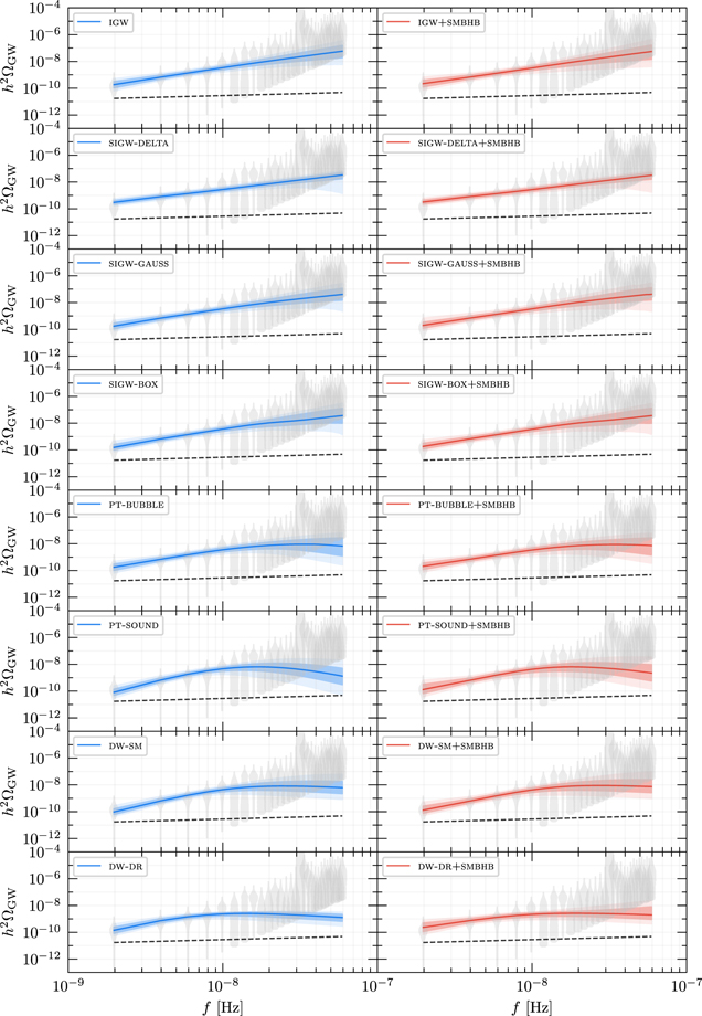
Figure 19. Median GWB spectra (solid lines) for all new-physics models considered in this work except for the cosmic-string models, together with their 68% and 95% posterior envelopes. Median GWB spectra for the cosmic-string models are shown in Figure 20. In the left column (blue shading), we show the median GWB spectra for the new-physics models alone; in the right column (red shading), we combine the new-physics signals with the signal from SMBHBs. The gray violins are symmetrical representations of the 1D marginalized posterior probability density distributions of the GW energy density at each sampling frequency of the data. The dashed black lines show the GWB spectrum produced by inspiraling SMBHBs (see caption of Figure 3).
Download figure:
Standard image High-resolution image
Figure 20. Same as Figure 19, but for the cosmic-string models considered in this work. See Appendix B for details.
Download figure:
Standard image High-resolution imageWe stress that the median GW spectra in Figures 3, 4, 19, and 20 represent effective power spectra that encapsulate global properties of the underlying distributions of actual GW spectra. In general, no individual GW spectrum at a given point in parameter space will exactly coincide with the median GW spectrum. For most models, the difference between the individual GW spectra and the median GW spectrum is rather mild. However, for some models, there can be noticeable differences, such as in the case of the SIGW models. Note, e.g., that the median GW spectrum of the sigw-delta model in Figure 4 does not have the characteristic double-peak structure that each individual GW spectrum in this model has. The reason for this is clear: the median GW spectrum follows from a distribution of many individual GW spectra whose peaks are located at different frequencies. The double-peak structure of the GW signal in the sigw-delta model is therefore washed out owing to the averaging over many individual GW spectra.
Another caveat is that median GW spectra violating an experimental bound (e.g., the LVK bound) do not automatically indicate that the corresponding model is ruled out. Again, as the median GW spectrum is constructed from a distribution of individual GW spectra, the violation of an experimental bound merely signals that some (maybe most) individual GW spectra are in conflict with the experimental data. It is, however, well possible that some fraction of the underlying distribution of individual GW spectra is not ruled out and is perfectly consistent with all experimental constraints. This is, e.g., true for the GW spectra from cosmic superstrings. The median GW spectrum of the super model violates the LVK bound (see Figure 4). However, at the level of the model parameter space, this merely means that some parameter regions are experimentally ruled out, while other regions remain viable (see Figure 11). Another example is the median GWB spectrum of the igw model, which appears to violate the Neff bound if it is extended to high frequencies beyond the NANOGrav band (see Figure 4). However, the igw model as a whole is not ruled out, as one can still choose the number of e-folds during reheating, Nrh, for each individual GW spectrum. In some regions of parameter space, the Neff bound then persists to pose a problem, despite this additional parametric freedom and even in the limit Nrh → 0; other regions, however, remain phenomenologically viable (see Appendix C.1 and Figure 22).

Figure 21. Same as Figure 5, but including the SMBHB parameters ABHB and γBHB. The black dashed lines in the three lower right panels show the prior distributions for ABHB and γBHB, i.e., one 2D Gaussian and two 1D Gaussian distributions.
Download figure:
Standard image High-resolution imageAppendix C: Supplementary Material
C.1. Cosmic Inflation
In Figure 22, we present constraints on the parameter space of IGWs, i.e., the igw model discussed in Section 5.1. This parameter space is spanned by four quantities: the tensor-to-scalar ratio r, the spectral index of the primordial tensor power spectrum nt
, the reheating temperature Trh, and the number of e-folds during reheating Nrh. However, because of the strong covariance between nt
and r in Figure 5, we are able to eliminate r and work on the 3D hypersurface in parameter space where r is given by the linear fit in Equation (22). The effective parameter space spanned by Trh, nt
, and Nrh is then subject to two constraints: (i) the upper limit on the allowed amount of extra relativistic radiation, ΔNeff, at the time of BBN and CMB decoupling (see Equation (23)), and (ii) the upper limit on the amplitude of the SGWB set by the LVK Collaboration based on their first three observing runs (see Equation (24)). The Neff bound can be saturated for a critical value of the cutoff frequency fend in the GW spectrum, which, for given Trh, is solely controlled by the Hubble rate at the end of inflation, Hend. This means that the Neff bound can be translated to a maximally allowed cutoff frequency  , which can then be converted to a maximally allowed Hubble rate
  and ultimately an upper limit
  on the allowed number of e-folds during reheating. Similarly, if the predicted GW signal at flvk = 25 Hz should exceed the LVK bound, we can derive upper limits
  and
and  by requiring fend not to exceed the lower end of the LVK band; for definiteness, we use
  .
.

Figure 22. Constraints on the parameters of IGWs, i.e., the igw model discussed in Section 5.1. The black solid lines refer to the Neff bound, while the maroon dashed lines refer to the LVK bound. The left panel shows the results for  , while the right panel compares
  to the duration of reheating that one would naively expect in models of standard single-field slow-roll inflation. The blue points correspond to the sampled points used to obtain the 2D marginalized posterior probability density for the model parameters Trh and nt
in Section 5.1. See Appendix C.1 for details.
to the duration of reheating that one would naively expect in models of standard single-field slow-roll inflation. The blue points correspond to the sampled points used to obtain the 2D marginalized posterior probability density for the model parameters Trh and nt
in Section 5.1. See Appendix C.1 for details.
Download figure:
Standard image High-resolution imageOur results for  obtained in this analysis are presented in Figure 22 in terms of black and maroon contour lines, where the black solid lines refer to the Neff bound, while the maroon dashed lines refer to the LVK bound. In the left panel we show our results for
  itself, while in the right panel we compare
  to the duration of reheating that one would naively expect in models of standard single-field slow-roll inflation (see Equations (15) and (16)),
where  denotes the minimal Hubble rate that is necessary to realize the desired value of Trh after inflation,
In other words, for given Trh,  represents the Hubble rate in the limit of instantaneous reheating, Nrh = 0. In terms of the maximally allowed number of e-folds
  and the naive expectation
  , we can then construct
which is the quantity shown in the right panel of Figure 22. In addition to the contour lines for  and ΔNrh, we also display the samples in the Trh–nt
plane that we obtain from our MCMC chains. The density of these blue points approximates the 2D marginalized posterior probability density for the model parameters Trh and nt
.
and ΔNrh, we also display the samples in the Trh–nt
plane that we obtain from our MCMC chains. The density of these blue points approximates the 2D marginalized posterior probability density for the model parameters Trh and nt
.
In view of the results in Figure 22, we can draw several conclusions: (i) Both the Neff bound and the LVK bound are only relevant at large values of the spectral index. At Trh ∼ 10−3 GeV, the number of e-folds during reheating is only constrained as long as nt
≳ 2.5, while at Trh ∼ 103 GeV, the bounds on Nrh only appear at nt
≳ 1. At f ≫ frh, these nt
values translate to a slope of the GW spectrum α in the range from α ∼ −1 to α ∼ 0.5, which is in the regime where we expect the approximate expression in Equation (25) to be valid (see also the discussion in Kuroyanagi et al. 2015). (ii) The LVK bound only depends on Trh. This follows from the fact that it is derived from the requirement  , which is independent of r and nt
. Typically, the LVK bound on Nrh is much weaker than the Neff bound on Nrh; only in the parameter region where the Neff bound begins to disappear,
, which is independent of r and nt
. Typically, the LVK bound on Nrh is much weaker than the Neff bound on Nrh; only in the parameter region where the Neff bound begins to disappear,  , does the LVK bound become competitive. (iii) The Neff bound is particularly strong at large reheating temperatures and large values of the spectral index, where
  can become even negative. This region, which we indicate by a dark-gray shading, is phenomenologically not viable and hence ruled out (see also the regions labeled Neff in Figure 5). In the excluded region, we also find ΔNrh ≪ 0, which indicates that reheating lasting for the naive number of e-folds
  will definitely result in a violation of the Neff bound. (iv) Farther away from the excluded region, the upper limits on Nrh become weak very fast,
  . In realistic models of inflation and reheating, where we typically expect
  , these bounds should be easy to satisfy. We therefore conclude that most of the region shaded in light gray, as well as the entire white region in Figure 22, can host viable realizations of the igw model. This includes, in particular, scenarios with a low reheating temperature, Trh ∼ 10−(3⋯0) GeV, and a large spectral index of the primordial tensor power spectrum, nt
∼ 3 ⋯ 4.
, these bounds should be easy to satisfy. We therefore conclude that most of the region shaded in light gray, as well as the entire white region in Figure 22, can host viable realizations of the igw model. This includes, in particular, scenarios with a low reheating temperature, Trh ∼ 10−(3⋯0) GeV, and a large spectral index of the primordial tensor power spectrum, nt
∼ 3 ⋯ 4.
In Figure 21, we show an extended version of the corner plot in Figure 5 including the SMBHB parameters ABHB and γBHB.
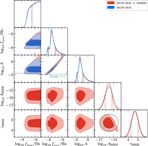
Figure 23. Same as Figure 6, but including the SMBHB parameters ABHB and γBHB.
Download figure:
Standard image High-resolution image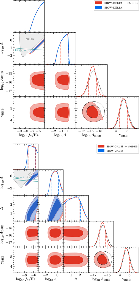
Figure 24. Same as Figure 7, but including the SMBHB parameters ABHB and γBHB.
Download figure:
Standard image High-resolution imageC.2. Scalar-induced Gravitational Waves
The generation of SIGWs relies on enhanced scalar perturbations on small scales, which can simultaneously lead to the production of PBHs. The parameter space of the SIGW models considered in this work is therefore subject to the constraint that the PBH mass density must not exceed the relic density of DM, fPBH ≤ 1 (see Equation (32)). This appendix explains how we evaluate this bound on the SIGW model parameters. We use the Press–Schechter formalism for spherical collapse (Press & Schechter 1974; Carr 1975) and mainly follow Inomata et al. (2017b) and Ando et al. (2018). The main quantity of interest is fPBH, which denotes the total fraction of PBH DM,

with PBH mass function f given as (Ando et al. 2018)
Here M is the mass of the PBH, T is the temperature at the time of PBH formation, γ is the ratio between the PBH mass and the horizon mass, and β(M) is the PBH production rate. In this work, we only focus on PBHs produced during the radiation-dominated era. We choose γ = 0.356, following Choptuik (1993), Koike et al. (1995), and Niemeyer & Jedamzik (1998), and assume that the mass of the PBH is proportional to the horizon mass when k = aH,
We can then express the PBH mass as a function of the temperature using the standard temperature–wavenumber relation in ΛCDM. Assuming that the density perturbation follows Gaussian statistics, β(M) is given by
where δc is the critical density perturbation for the PBH formation, whose exact value depends on the shape of the curvature power spectrum and satisfies 0.4 ≲ δc ≲ 0.6 (Musco et al. 2005, 2021), and σ2(M) is the variance of the coarse-grained density perturbation, which in the radiation domination era is given by
Here W(x) is some window function smearing over k−1 and
is the transfer function for the radiation-dominated era. In our work, we choose δc
= 0.45 as a fiducial value (Ando et al. 2018; Wang et al. 2019) and a Gaussian window function  .
.
Our analysis is subject to a few caveats. The correct value of the critical density δc depends on the choice of the power spectrum and the window function (Ando et al. 2018; Musco 2019; Young 2019; Escrivà 2020; Escrivà et al. 2020; Gow et al. 2021; Musco et al. 2021; Dandoy et al. 2023) and the nonlinear relation between density perturbations and density contrast (De Luca et al. 2019; Young et al. 2019; Escrivà 2020). In this work, we use a single value of δc for three different power spectra for computational reasons. We also disregard any corrections from the QCD equation of state, which are expected to be important at the frequency range probed by PTA observations (Abe et al. 2021; Escrivà et al. 2022a; Juan et al. 2022; Dandoy et al. 2023; Musco et al. 2023).
The statistics of the primordial scalar perturbations also strongly affect the abundance of PBHs since, in general, enhanced scalar perturbations come with different levels of non-Gaussianity. In this work, we focus on Gaussian primordial scalar perturbations. With non-Gaussianities, the same PBH abundance can be produced with scalar perturbations whose amplitudes are orders of magnitude smaller than those produced with Gaussian scalar perturbations. Therefore, primordial non-Gaussianity can dramatically affect the PBH bounds (Young & Byrnes 2013; Garcia-Bellido et al. 2017; Nakama et al. 2017; Pattison et al. 2017; Franciolini et al. 2018; Cai et al. 2019; De Luca et al. 2019; Young et al. 2019; Iacconi & Mulryne 2023). In the parameter region where SIGWs manage to explain the NANOGrav signal, this would notably aggravate the PBH overproduction problem, which means that sizable non-Gaussianities could completely rule out the SIGW interpretation of the signal. In this work, we also neglect evolutionary effects on the PBH mass function, namely accretion and mergers, where accretion effects are expected to be small for sub-solar-mass PBHs (Ali-Haïmoud & Kamionkowski 2017; Raidal et al. 2019; De Luca et al. 2020; Vaskonen & Veermäe 2020).
In summary, the final PBH DM fraction is quite sensitive to the assumptions discussed above. The bounds presented in the main text should be taken with a grain of salt owing to the uncertainties in the computation of fPBH.
In Figures 23 and 24, we show extended versions of the corner plots in Figures 6 and 7 including the SMBHB parameters ABHB and γBHB.
C.3. Cosmological Phase Transitions
In the phase transition analysis discussed in the main text, we allow the low-frequency spectral index to float despite that causality predicts a = 3. We do this to capture possible double-peak spectral features with our simple power-law parameterization. However, it is not clear whether or not a strong and fast phase transition like the one needed to explain the observed signal could produce such a double-peak structure (Hindmarsh et al. 2017; Hindmarsh & Hijazi 2019). Therefore, in Figure 25 we report the results of a phase transition analysis where we assume a = 3. Figure 25 shows the reconstructed posterior distributions for the parameters α*, T*, and H* R* of the pt-sound and pt-bubble models, both for the case where the PT is assumed to be the only source of GWs (blue contours) and for the scenario where we consider the superposition of the PT and SMBHB signal (red contours). For the analyses where the SMBHB signal is included, we also report the posterior distributions for ABHB and γBHB. For the pt-sound model we notice very minor differences compared to the analysis in the main text. However, for the pt-bubble model we notice how the posterior for T* is peaked to slightly smaller values for the reasons explained in the main text.
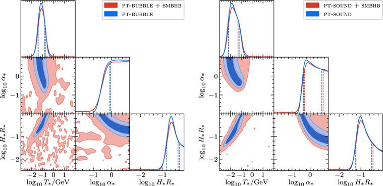
Figure 25. Same as in Figure 5, but for the pt-sound (left panel) and pt-bubble models with a low-frequency slope fixed to the value predicted by causality, i.e., a = 3.
Download figure:
Standard image High-resolution imageIn Figures 26 and 27, we report the posterior distributions for all the parameters of the phase transition models, including the spectral shape parameters a, b, and c that were excluded from Figure 8. As expected for the pt-bubble model, the low-frequency slope is peaked around a ∼ 2, which is the reconstructed slope of the GWB signal, while the posteriors for b and c are approximately flat. For the pt-sound model, the posterior for a is peaked around the lower limit of the prior range a = 3, and there is also a mild preference for larger values of the width parameter, as this would flatten the spectrum close to the peak.
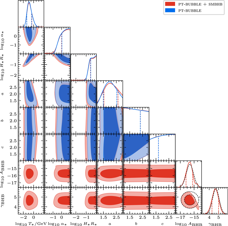
Figure 26. Same as Figure 8, but including the spectral shape parameters a, b, c and SMBHB parameters ABHB and γBHB.
Download figure:
Standard image High-resolution image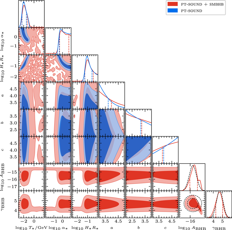
Figure 27. Same as Figure 26, but for the pt-sound model.
Download figure:
Standard image High-resolution imageC.4. Cosmic Strings
In our discussion of stable cosmic strings in the main text, we only present the reconstructed marginalized 1D posterior distributions for the dimensionless cosmic-string tension, G μ (see Figure 9). The four strings-plus-SMBHBs models stable-c+smbhb, stable-k+smbhb, stable-m+smbhb, and stable-n+smbhb, however, feature three model parameters in total: G μ, ABHB, and γBHB. In this appendix, we complement the discussion in Section 5.4 and show the corner plots for these parameters (see Figure 28). A notable feature of these corner plots is that the plateau region at small values of G μ, which we had already observed in Figure 9, now also appears in the form of flat directions in the 2D posterior distributions for G μ and ABHB, as well as for G μ and γBHB. Meanwhile, the 2D posterior distributions for ABHB and γBHB represent distorted versions of the 2D Gaussian prior distribution that we employ in our analysis, peaking at large ABHB and small γBHB, where SMBHBs yield the dominant contribution to the signal. All four corner plots in Figure 28 are qualitatively identical and only display slight numerical differences.

Figure 28. Posterior distributions for the stable+smbhb strings models including the SMBHB parameters ABHB and γBHB. We also report the marginalized  posterior distributions for the stable string models (blue lines).
Download figure:
Standard image High-resolution imageNext, let us turn to metastable strings. In the main text, we discuss the number density of closed string loops for the case of stable strings (see Equation (43)), as well as for metastable strings (see Equation (46)). In the meta-ls model, we need in addition the number density of string segments that form when long strings and closed loops break apart as a consequence of monopole nucleation. In order to compute the GW signal from segments, we use again Equations (40) and (42), where we replace the loop number density nl by the segment number density ns and the GW power spectrum Pk in Equation (41) by Pk = 4/k, which was derived by Martin and Vilenkin in the approximation of a straight string segment in Martin & Vilenkin (1997). Meanwhile, all relevant expressions for the segment number density ns were computed in Leblond et al. (2009) and Buchmuller et al. (2021), which we shall summarize in this appendix. For more details, we refer to Leblond et al. (2009) and Buchmuller et al. (2021).
First, we consider segments that form when long strings break apart. We denote their number density by  , which we decompose into three different contributions that are relevant at different times and in different parameter regimes,

Here  is the number density of segments that originate from long strings, assuming the scaling regime to end during radiation domination, evaluated during radiation domination and after the onset of the decay regime,
where  is the number density of segments that originate from long strings, assuming that the scaling regime ends during radiation domination, evaluated during matter domination and after the onset of the decay regime,
and  is the number density of segments that originate from long strings, assuming that the scaling regime ends during matter domination, evaluated during matter domination and after the onset of the decay regime,
In view of these expressions, several comments are in order: (i) Throughout our analysis, we assume that GW emission by segments is as efficient as GW emission by loops, i.e., we work with Γ = 50 for both loops and segments. (ii) All three expressions depend on the dimensionless correlation length of the long-string network, for which we use the attractor values in the VOS model, ξr
= 0.27 and ξm
= 0.63 during radiation and matter domination, respectively. (iii) For a given choice of parameter values,  ,
,  , and
, and  never contribute simultaneously to the segment number density. For teq > ts
only
never contribute simultaneously to the segment number density. For teq > ts
only  and
and  yield nonvanishing contributions (first
  at t < teq and then
  at t > teq), whereas for teq < ts
the number density of segments from long strings is solely determined by
at t > teq), whereas for teq < ts
the number density of segments from long strings is solely determined by  at all times t > ts
.
at all times t > ts
.
In addition to segments from long strings, there is also a population of segments that form when closed string loops begin to break apart because of monopole nucleation. We denote the number density of this population by  , where the index refers to the fact that
  only describes the first generation of segments that form when closed loops break apart for the first time. This first generation then gives rise to a second generation of segments that follow from monopole nucleation on first-generation segments, and so on and so forth. We comment on these higher generations further below. Before that, however, we discuss
  , which we decompose again into three contributions,

Here  is the number density of first-generation segments that originate from closed loops that formed during radiation domination, evaluated during radiation domination and after the onset of the decay regime,
where  is the number density of first-generation segments that originate from closed loops that formed during radiation domination, evaluated during matter domination and after the onset of the decay regime,
and  is the number density of first-generation segments that originate from closed loops that formed during matter domination, evaluated during matter domination and after the onset of the decay regime,
where F2 and F1 are shorthand notations for the following expressions involving the hypergeometric function 2 F1:
These results were derived in Buchmuller et al. (2021) based on the loop number densities in the so-called BOS model (Blanco-Pillado et al. 2014), which explains the occurrence of factors such as 0.27, 0.45, and 0.31 in Equations (C17) and (C18) (see Buchmuller et al. 2021 for more details).
Finally, the expressions in Equations (C15), (C16), and (C17) enable us to estimate the total number densities of all generations of segments that descend from closed loops breaking apart because of monopole nucleation. In principle, these number densities are described by a partial integro-differential equation where the abundance of the nth segment generation acts as a source term for the (n + 1)th generation. Formally, this partial integro-differential equation can be solved analytically in terms of an infinite recursive series (Buchmuller et al. 2021). The numerical evaluation of this series is, however, technically demanding, which is why we choose to follow a different approach for the purposes of this paper. As shown in Buchmuller et al. (2021), it turns out that the total number densities for segments from closed loops result in predictions for the GW spectrum that are very similar to those obtained from the corresponding first-generation number densities in Equations (C15), (C16), and (C17)—up to a numerical fudge factor of  . At the level of the number densities, it therefore suffices to rescale all first-generation number densities by a constant factor in order to obtain effective number densities for all generations of segments that descend from closed loops breaking apart,
We stress that the functional dependence on ℓ and t is typically not the same for the first-generation and total number densities; the rescaling in Equation (C20), however, achieves comparable results at the level of the GW spectrum. In our analysis, we consistently use a fudge factor of 5, which is a characteristic value across large regions of parameter space.
In Figures 29 and 30, we show extended versions of the corner plots in Figures 10 and 11 including the SMBHB parameters ABHB and γBHB.
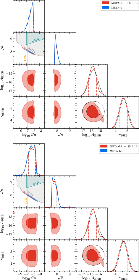
Figure 29. Same as Figure 10, but including the SMBHB parameters ABHB and γBHB.
Download figure:
Standard image High-resolution image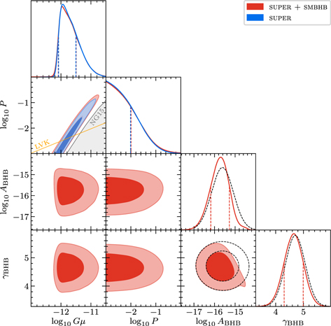
Figure 30. Same as Figure 11, but including the SMBHB parameters ABHB and γBHB.
Download figure:
Standard image High-resolution imageC.5. Domain Walls
In Figure 31, we report the posterior distribution for all the parameters of the domain wall models, including the spectral shape parameters b and c that were excluded from Figure 12. For both the dw-sm and dw-dr models we find a flat posterior for the high-frequency slope, b. This result is expected since most of the low frequency bins are fit by the low-frequency tail of the spectrum. For the width parameter, c, instead, both models prefer values near the upper range of our prior range. This preference for wider spectra derives from a mismatch between the reconstructed slope of the GWB, a ∼ 2, and the one predicted by causality, a ∼ 3. Larger width parameters make the spectrum from domain walls flatter near the peak and allow for a better fit to the data.
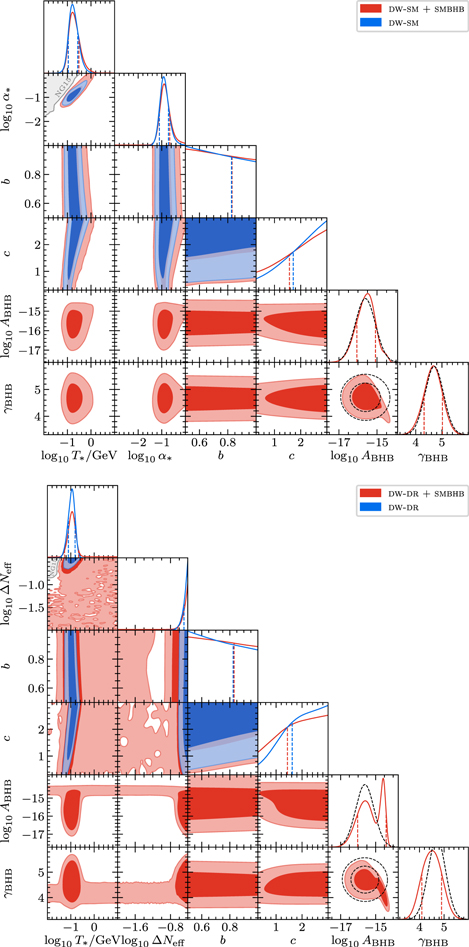
Figure 31. Same as Figure 12, but including the spectral shape parameters b, c and the SMBHB parameters ABHB and γBHB.
Download figure:
Standard image High-resolution imageC.6. Dark Matter Substructures
In this appendix we provide more details on the procedure that we followed to derive the constraints on fPBH reported in Section 6.2.
Given a PBH with position relative to the pulsar given by r (t) = r 0 + v t, where r 0 and v are the initial PBH position and velocity, respectively, we can write the Doppler and Shapiro signals as


where xD ≡ (t − tD,0)/τD and xS ≡ (t − tS,0)/τS. These expressions only include cubic terms in time t and have been previously derived in Dror et al. (2019) and Lee et al. (2021b). For the static limit in which τ ≫ Tobs, these expressions can be expanded in series of t0/τ. Since the  terms would be degenerate with the timing model, the measurable new-physics signal can then be parameterized as a term ∝t3 as
where AD(S),sta for both the Doppler and Shapiro static signal cases are dimensionless amplitudes given by
For the Doppler case, in the dynamic limit when τ ≪ Tobs, the dominant contribution would come from the first term in Equation (C21) where  . Up to linear order in xD, we can write

where AD,dyn is the dimensionless amplitude given by

Given the expressions in Equations (C21) and (C22) for the Doppler and Shapiro signals, we use the MC developed in Lee et al. (2021a) to derive the distributions  . Specifically, we proceed as follows:
- 1.For each pulsar we generate a population of NPBH PBHs, where NPBH is implicitly defined by the relationwhere the simulation volume, V, is a sphere of radius centered around the pulsar position for the Doppler signal and a cylinder with the same radius and height given by the Earth−pulsar distance for the Shapiro signal. Here is the average PBH velocity, and Tobs,I
is the observation time of the Ith pulsar.
- 2.For each of these PBHs we generate a random initial position and velocity. Since PTA searches are only sensitive to DM subhalos in the neighborhood of the solar system, we expect the position distribution to be uniform. Therefore, we use the probability density function f( r ) = 1/V to sample initial positions. To sample PBHs' velocity, we use a Maxwell–Boltzmann distribution with v0 = 325 km s−1, vesc = 600 km s−1, and the angular dependence assumed to be isotropic.
- 3.The PBHs' signals are then classified as dynamic if they satisfy the condition Tobs,I − τ > t0 > τ and static otherwise.
- 4.To evaluate Astat, we sum the static signals of all PBHs computed by using Equations (C21) and (C22), and we fit the resulting signal to a cubic polynomial in time to extract the t3 term. To compute AD,dyn, we take the closest transiting object and compute the signal amplitudes using Equation (C27).


All the previous points are repeated for 2.5 × 10³ realizations to obtain the distributions  . Given the conditional distributions
  and the posterior distribution
  derived by analyzing our data, we can write
Then, using Bayes's theorem, we can rewrite
Our priors on  and
and  are uniform, which allows us to eventually write Equation (C29) as
where the ∝ implies that the p(fPBH∣
δ
t
) would be subject to the normalization condition,  .
.
In the presence of a DM−baryon fifth force in the form of a Yukawa potential in Equation (72), assuming point-mass DM, the pulsar frequency shift due to Doppler effect is given by (Gresham et al. 2023)
The integral in Equation (C32) has to be computed numerically, and the signal due to the fifth force can be computed by performing an additional integration over time and subtracting away degeneracies with timing model parameters. The total signal is the sum of the gravitational and the fifth-force contribution, hD,total(t) = hD,fifth(t) + hD(S)(t). In this analysis of the fifth-force constraint, we only consider the scenario where the DM substructure makes up the entirety of the DM local density, which is equivalent to taking fPBH = 1 for the gravitational contribution. Parameterizing the signal as  similar to the PBH case, the amplitude AD,total is a random variable dependent on λ and
  . The probability distribution function
  can be extracted again by Monte Carlo simulations and Bayes's theorem. Finally, the posterior distribution of
  and λ,
  , is given by the analog of Equation (C31),
Footnotes
- 81
The noise in the 95% credible interval for the nt –
posterior distribution of the igw+smbhb model is due to the presence of an extended plateau region in the posterior distribution, which renders the kernel density reconstruction sensitive to Poisson fluctuations in the binned MCMC data. - 82
The scalar field can either be an elementary field of a weakly coupled theory or correspond to the vacuum condensate of a strongly coupled theory. Scenarios with several scalars are also possible.
- 83
Turbulent motion of the plasma can also source GWs; however, its contribution is usually subleading compared to the two other contributions (see the discussion in Caprini et al. 2020). Therefore, we ignore GWs sourced by turbulence in our analysis.
- 84
Causality fixes the spectral index of the phase transition GWB signal to a = 3 in the low-frequency limit. However, given the simple power-law parameterization adopted in this work, double-peak features observed in the results of numerical simulations (Hindmarsh et al. 2017; Hindmarsh & Hijazi 2019) can appear as a deviation from this behavior near the peak frequency. Nonetheless, in Appendix C.3, we also report the results of an analysis in which the low-frequency slope is fixed to a = 3.
- 85
The noise in the 95% credible regions of the posterior distributions of the pt-sound+smbhb model is due to the presence of an extended plateau region in the posterior distribution, which renders the kernel density reconstruction sensitive to Poisson fluctuations in the binned MCMC data.
- 86
In the case of the four strings-plus-SMBHBs models, the probability density threshold for this procedure may coincide with the height of the plateau at low frequencies. If this happens, sampling fluctuations in the plateau region will lead to a set of disjoint intervals. To avoid these fictitious intervals, we set the upper limit where the posterior probability density falls to the level of the plateau and adjust the lower limit within the plateau so that the intervals contain 95% of the posterior probability.
- 87
In our analysis, we work with the upper limit on the amplitude of a generic isotropic and stochastic GWB that was reported by the LVK Collaboration in Abbott et al. (2021a). Combining this limit with our own GW spectra, we find G μ ≲ 2 × 10⁻⁷. This bound needs to be compared to the results of Abbott et al. (2021b), a dedicated search for GWs from stable cosmic strings by the LVK Collaboration. The analysis in Abbott et al. (2021b) models the GW spectrum from cosmic strings based on slightly different assumptions. Model A in Abbott et al. (2021b) is, however, similar to our approach and leads the same bound on G μ in the limit of a large number of kinks, Nk ≫ 1 (see the panel for model A in Figure 3 of Abbott et al. 2021b at Nk ∼ 100 ⋯ 200).
- 88
- 89
Here we focus on signals from scalar (spin-0) and vector (spin-1) ULDM. We leave the search for the effects of spin-2 ULDM (Marzola et al. 2018; Armaleo et al. 2020a, 2020b; Xia et al. 2023) to future work. For scalar DM, i is absent, since the field has only one component. For vector DM, i ∈ {1, 2, 3} for each massive vector polarization.
- 90
A similar approach could be applied to set constraints on the local abundance of DM subhalos. However, we do not consider this case, since our constraints for PBHs are already quite weak. Constraints on DM subhalos would likely be even weaker, making it a less promising target for future PTAs.
- 91
From now on, we suppress the PBH mass, M, in the expressions for the conditional probabilities for the sake of notation.


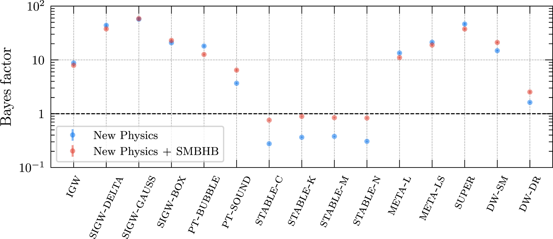
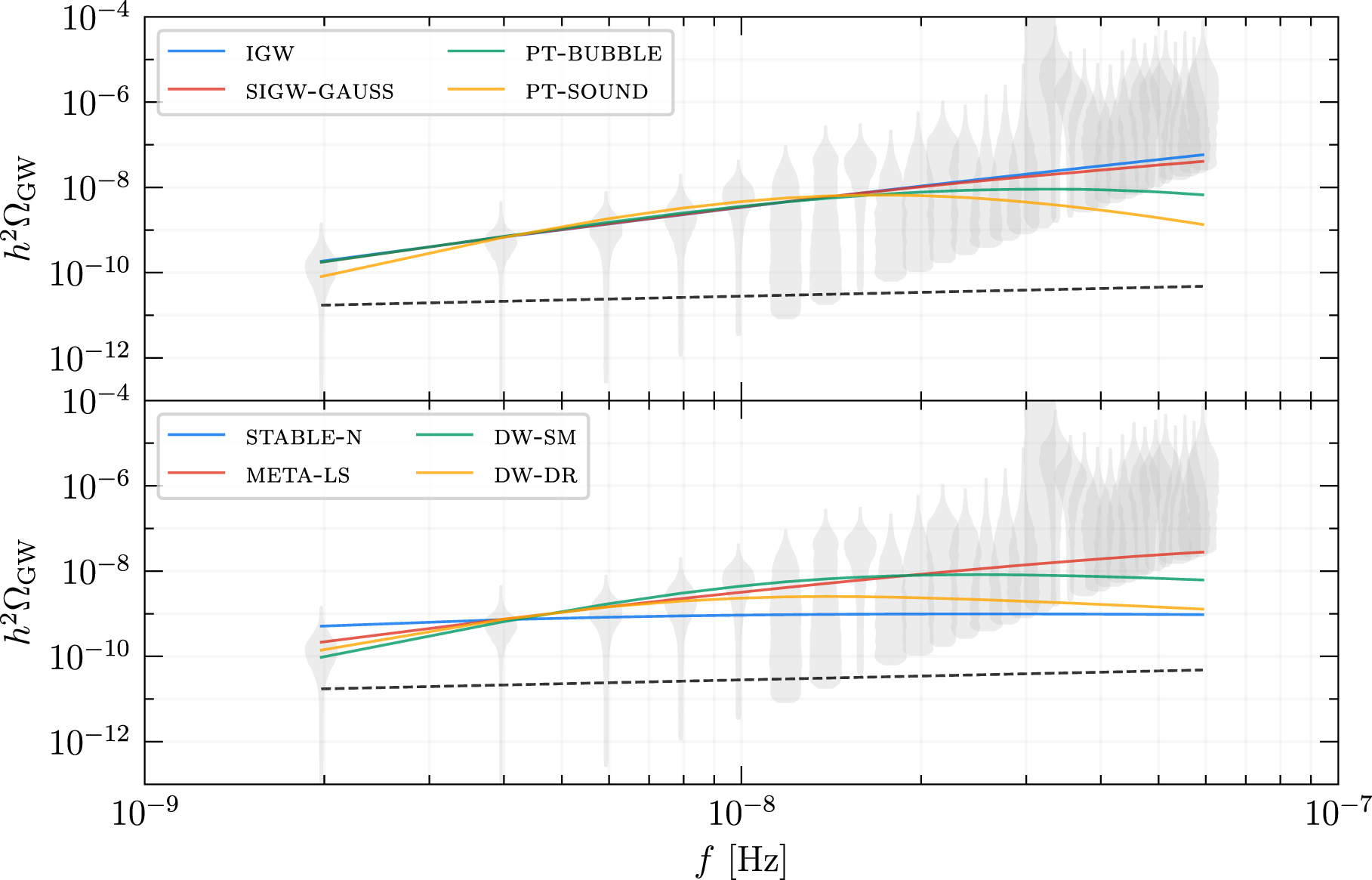
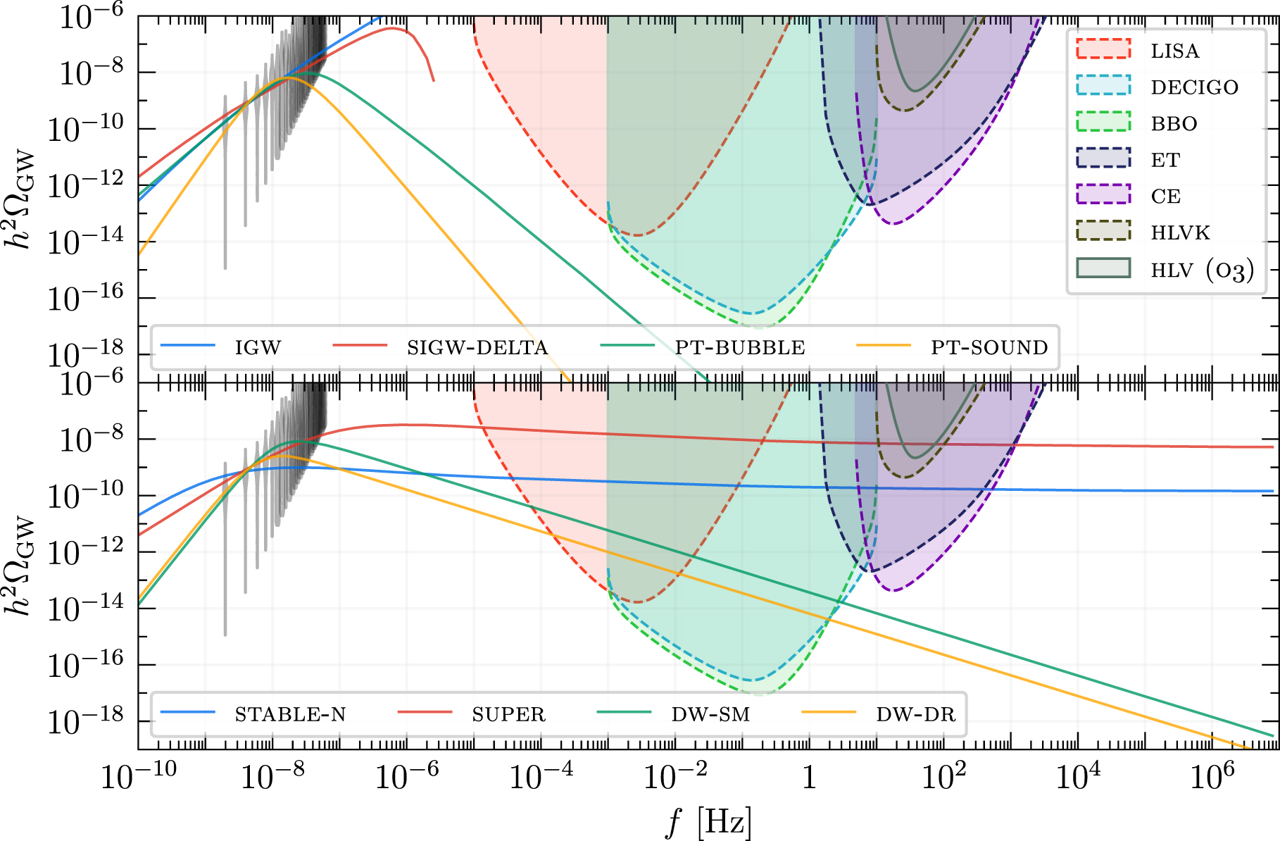
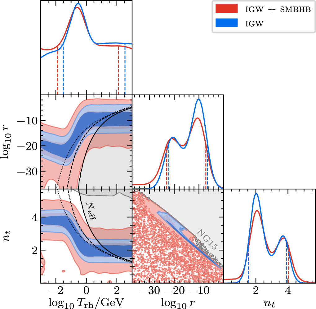
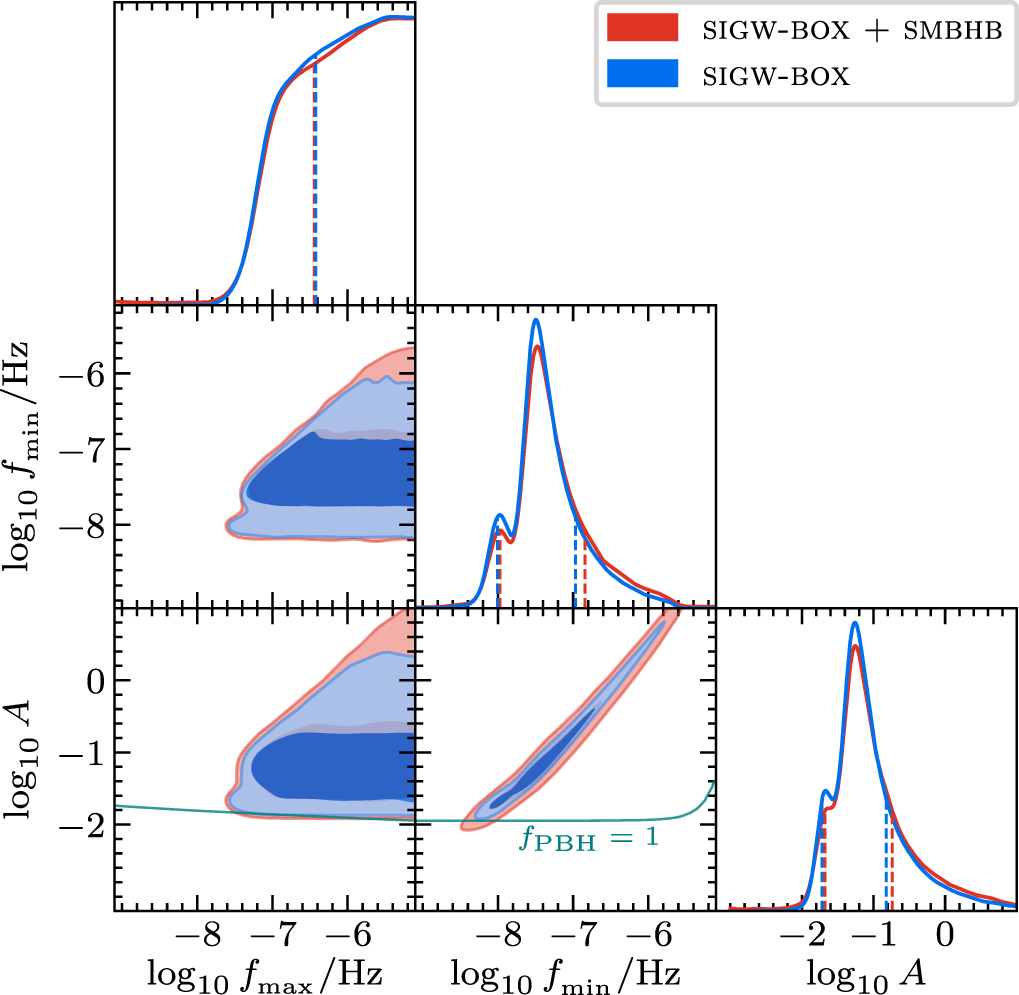
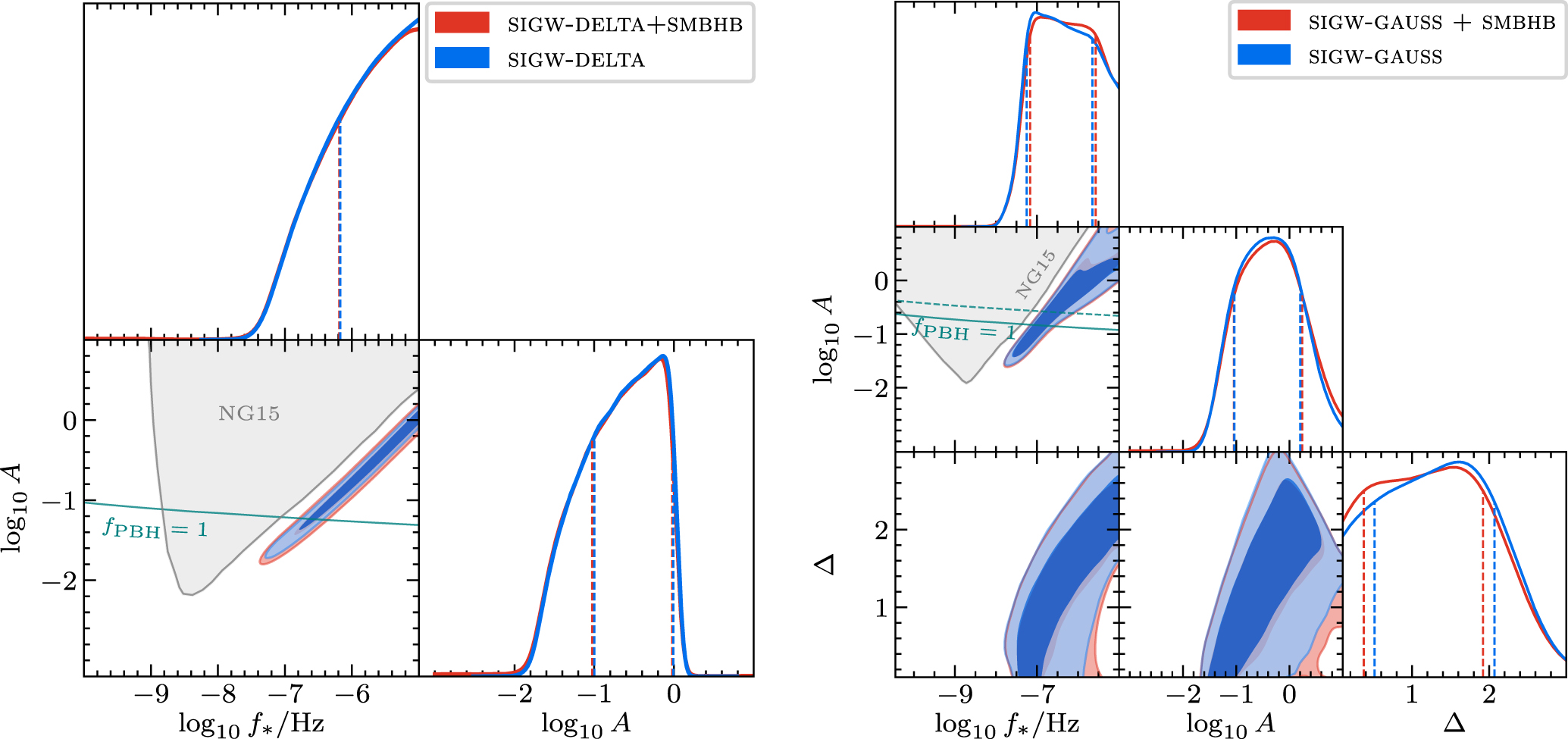
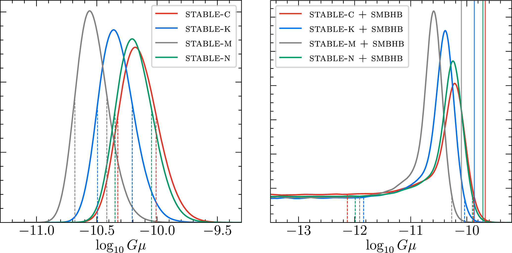
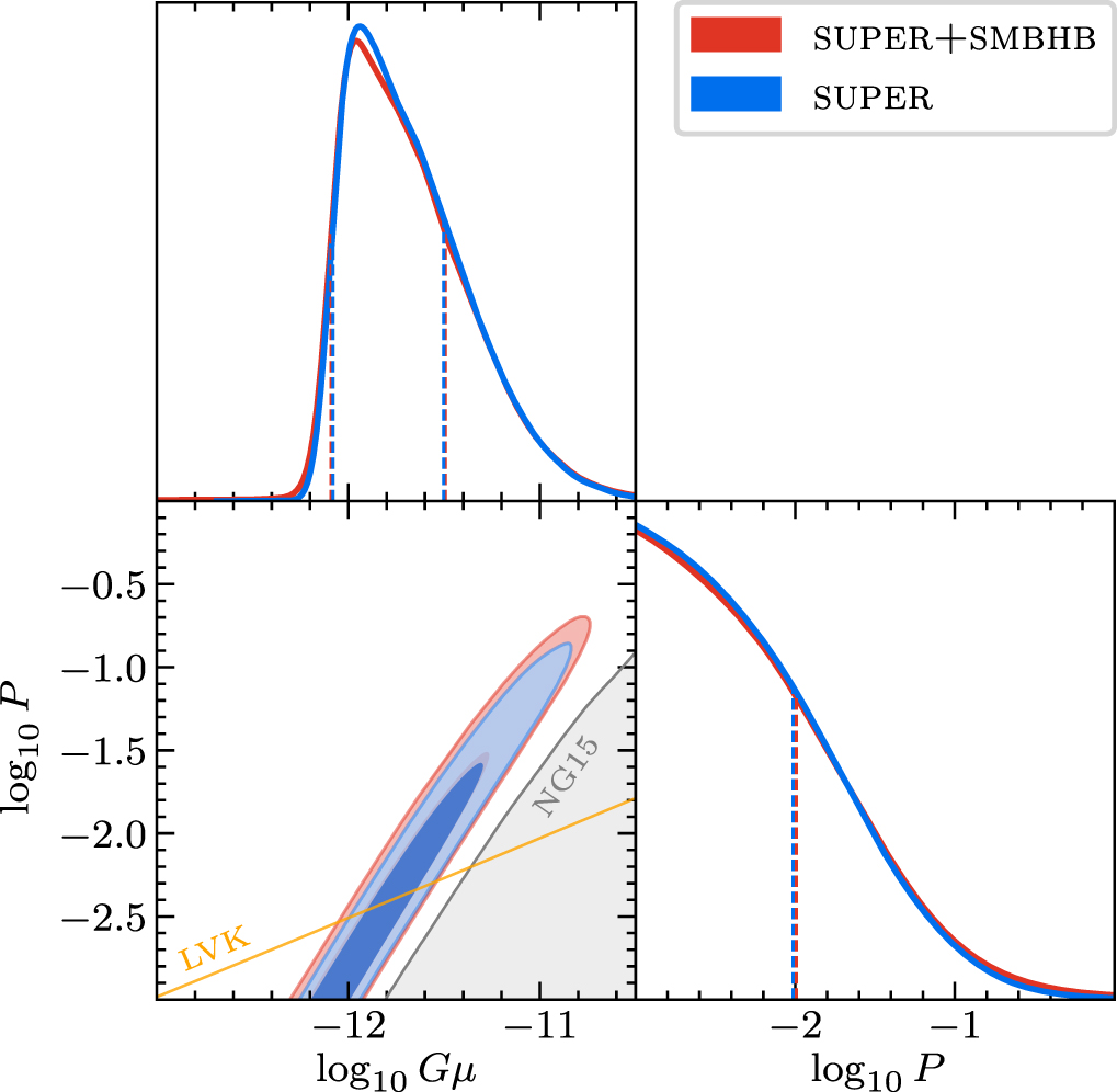
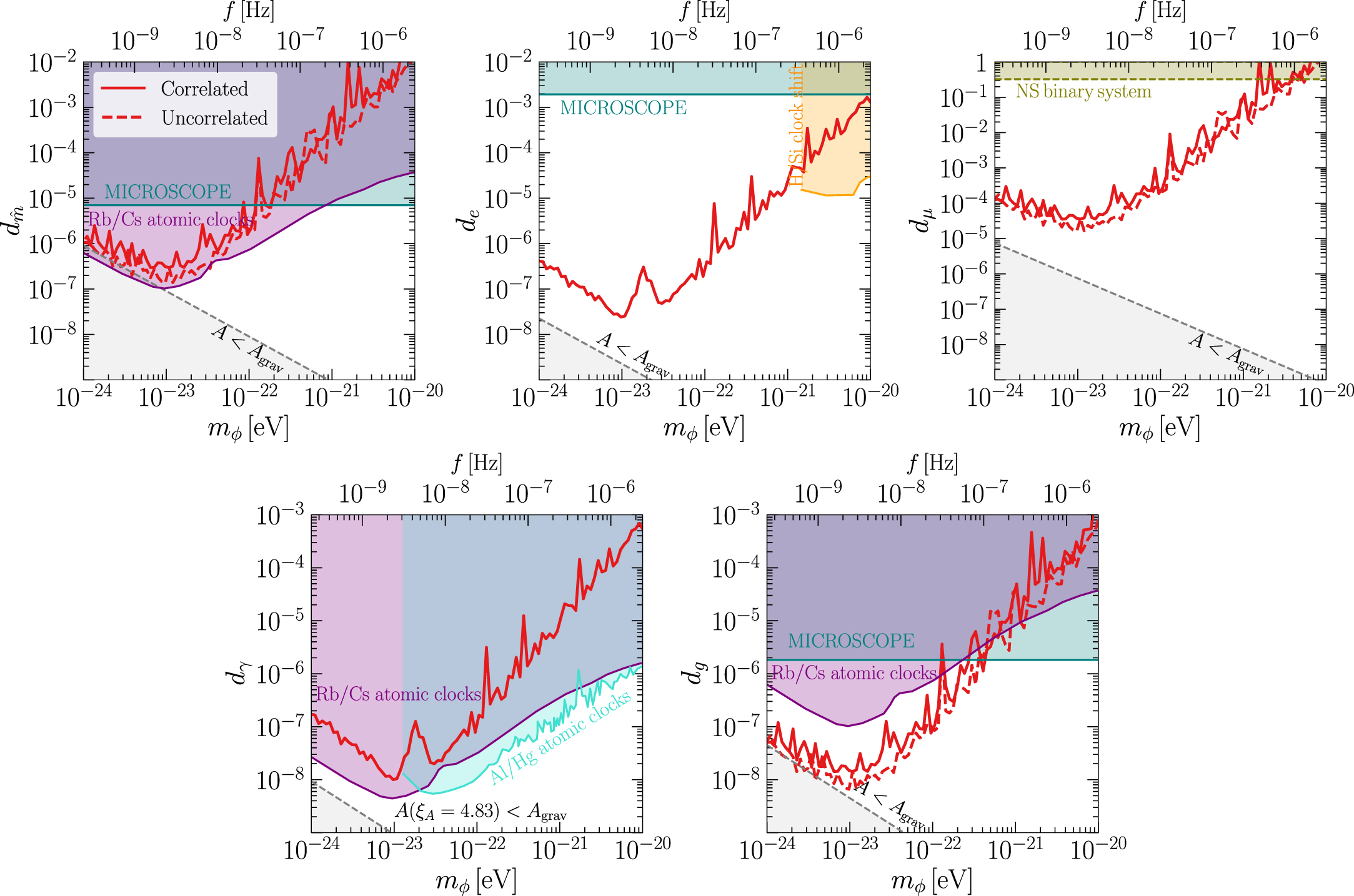
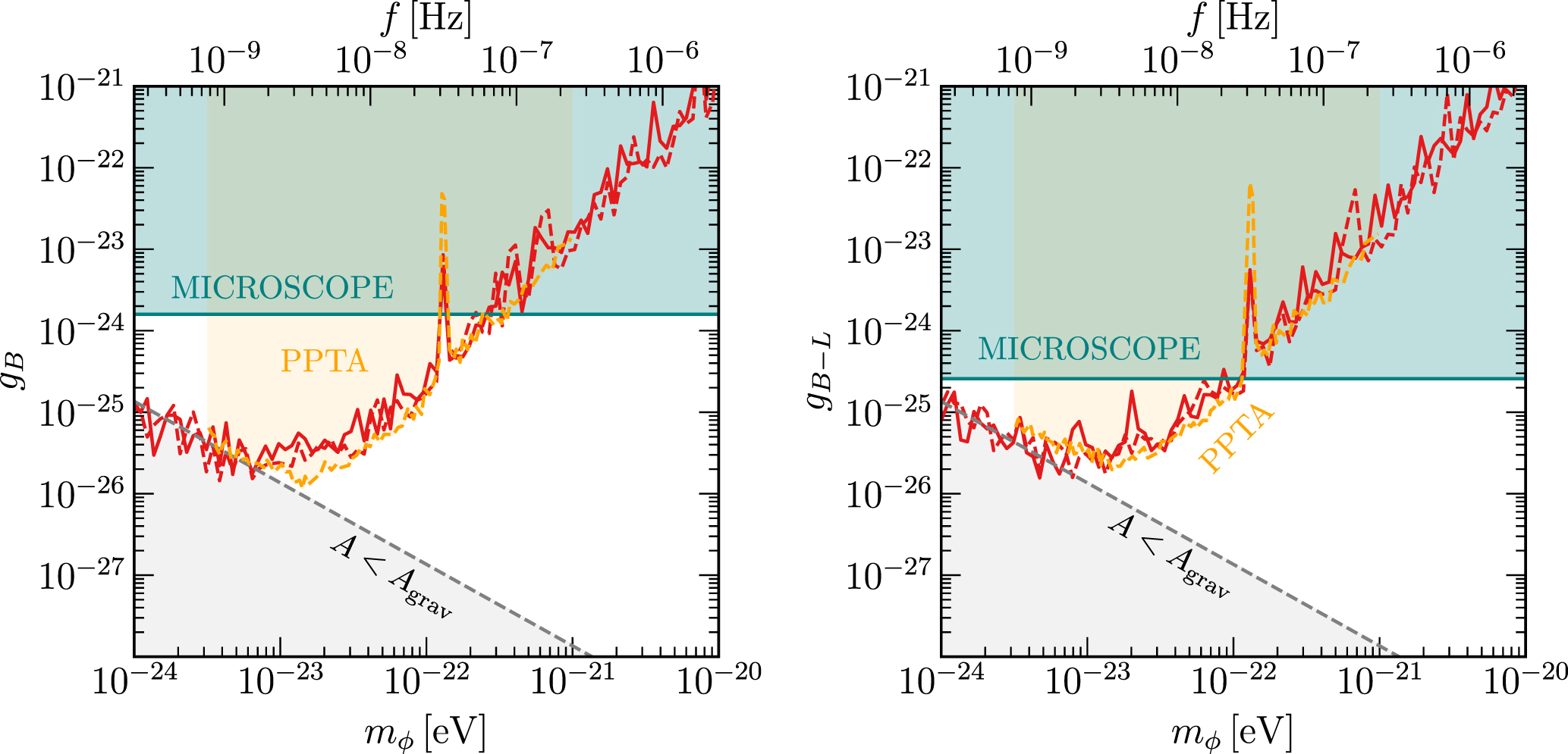
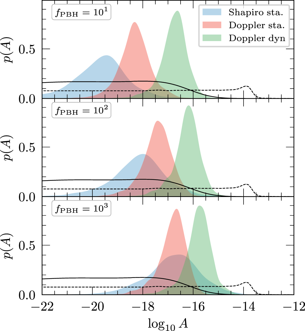
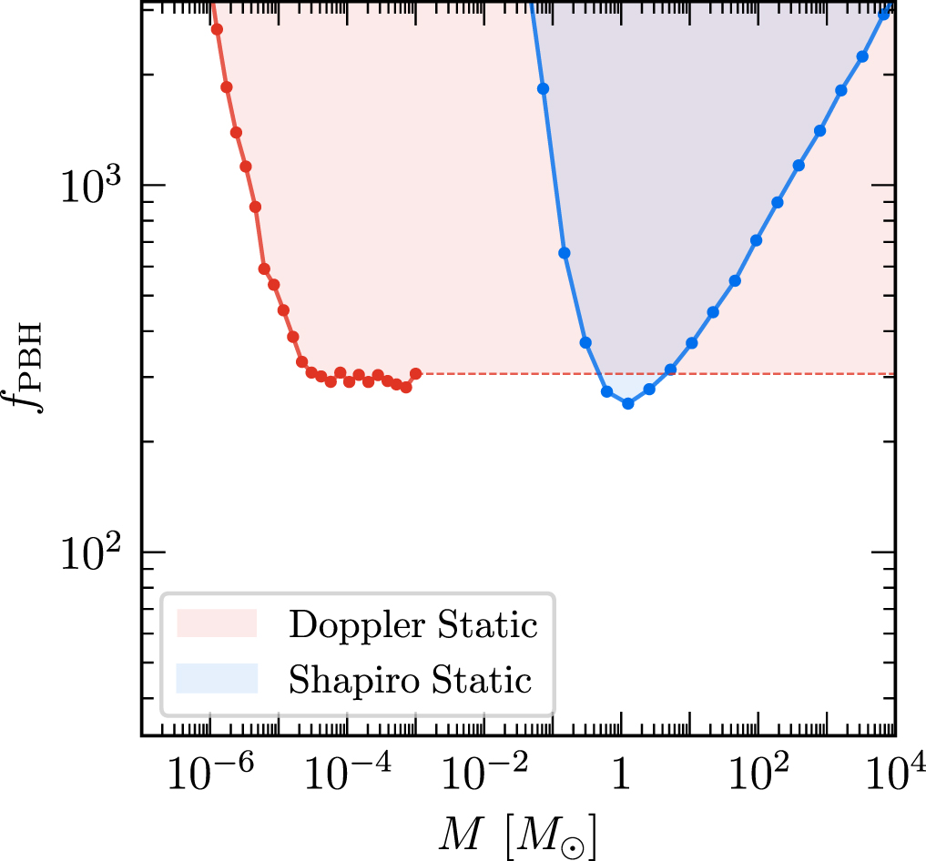
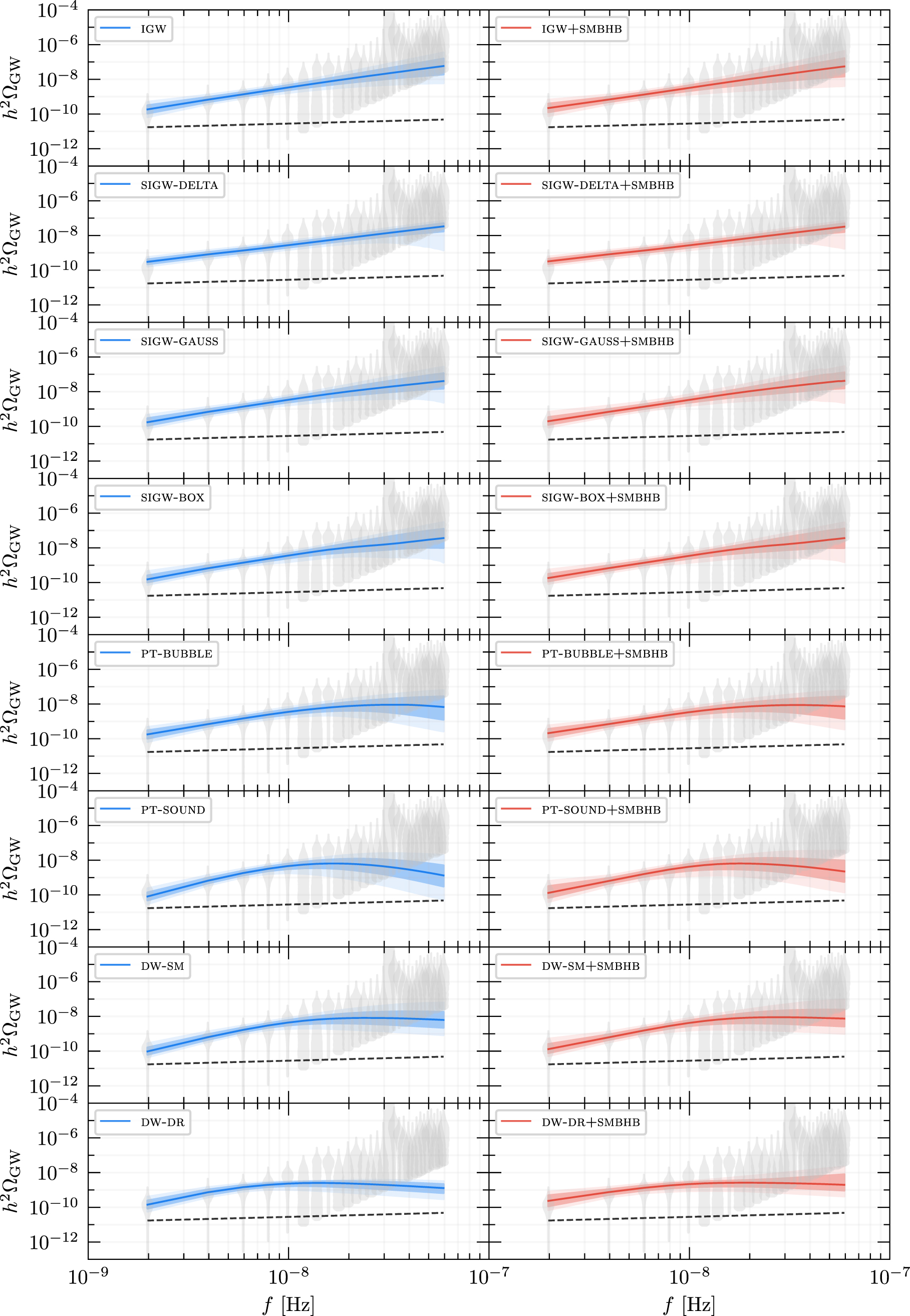
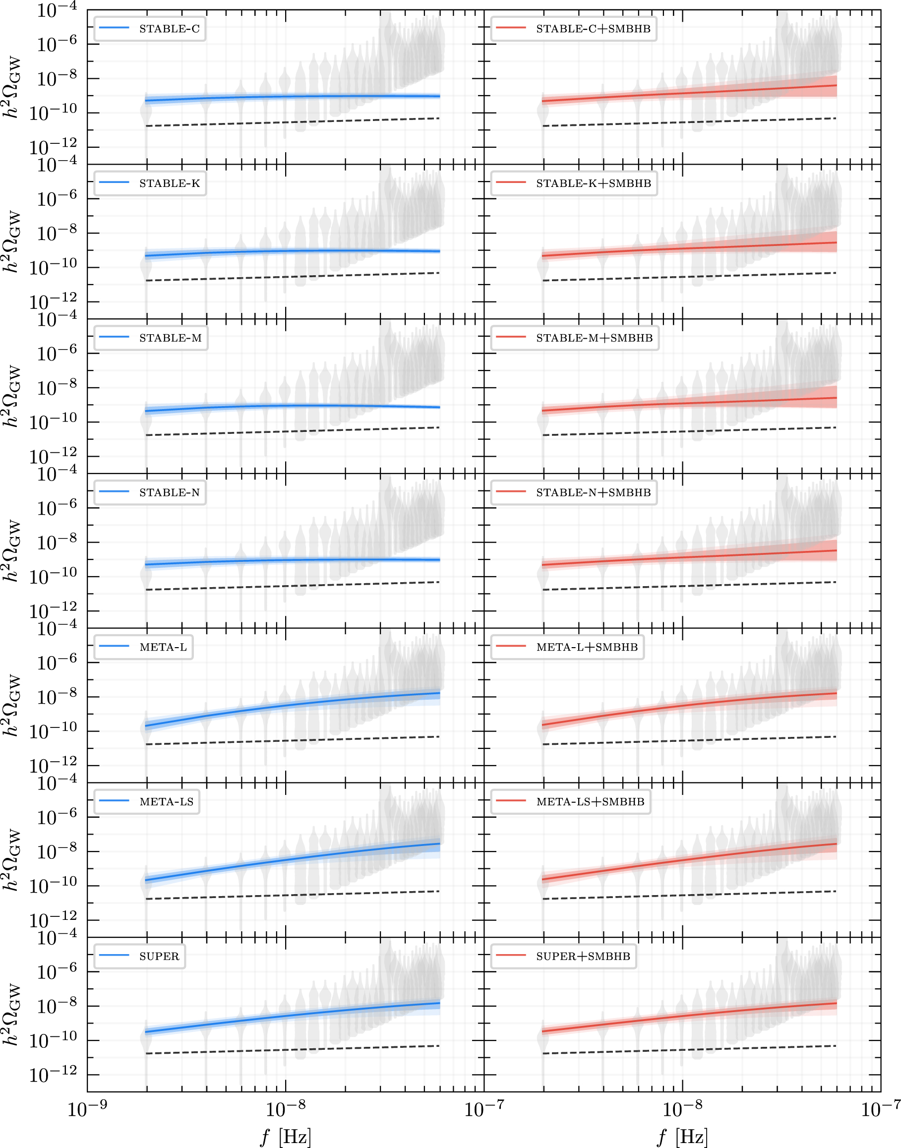
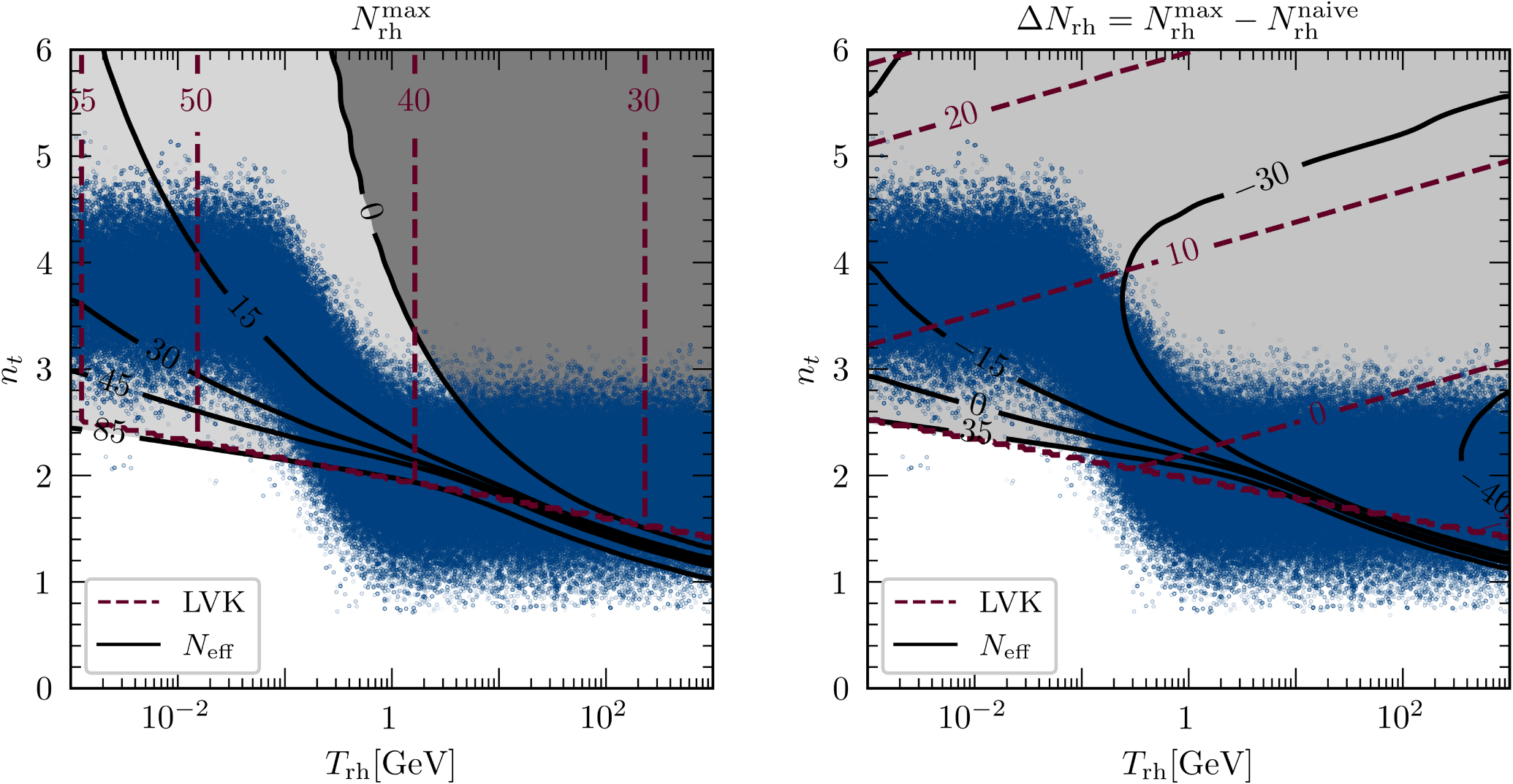
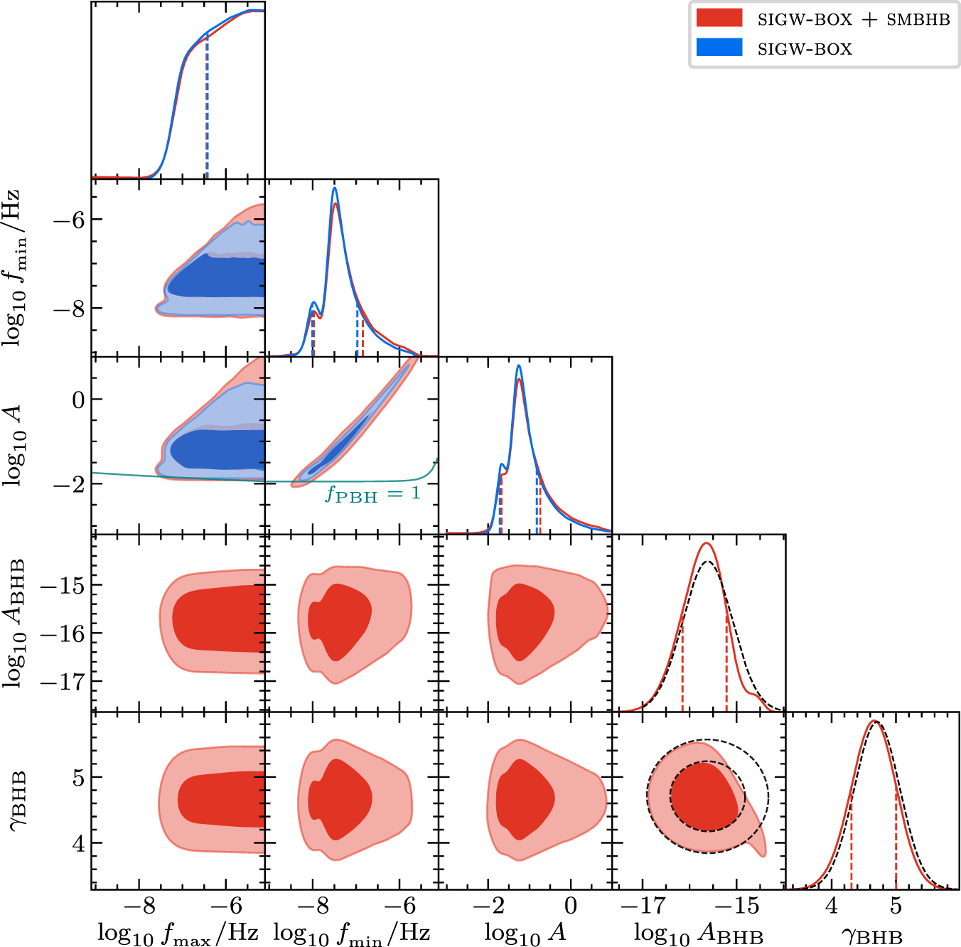
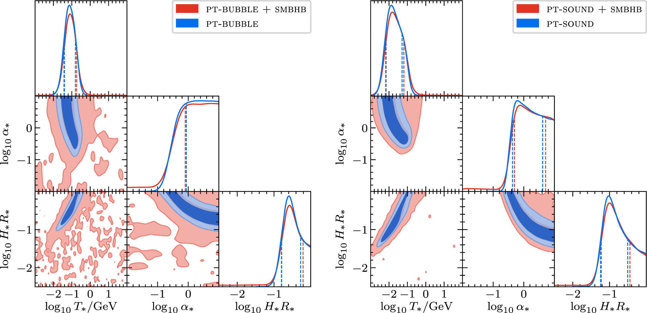