Discovery of the 5 keV Cyclotron Line Followed by Three Harmonics in Swift J1626.6-5156

Swift J1626.6–5156 is a transient X-ray pulsar (XRP) with a spin period of ∼15 s discovered on 2005 December 18 by the Swift Burst Alert Telescope (BAT) during a giant outburst (Krimm et al. 2005). The outburst lasted for approximately half a year and was followed by a longer period of a few years during which the object remained active and strongly variable on timescales from 45 to 95 days (Reig et al. 2008; Baykal et al. 2010).

The most complete study of the system to date has been conducted by Reig et al. (2011), who, based on multi-frequency observations, concluded that Swift J1626.6–5156 is a Be/X-ray binary (BeXRB) with a B0Ve companion located at a distance of D ∼ 10 kpc. This estimate is rather uncertain, and the Gaia Third Early Data Release (EDR3) estimates are in the range of 5.8–12 kpc (Bailer-Jones et al. 2021). Here we adopt 10 kpc distance for easier comparison with previous results. The counterpart (2MASS16263652-5156305) shows strong Hα emission (Negueruela & Smith 2006), typical of a Be star. The ∼15.3 s spin period of the neutron star (Markwardt & Swank 2005; Palmer et al. 2005) and the 132.9 days orbital binary period (Baykal et al. 2010) are also typical for Be-systems (see e.g., Corbet 1986). At the same time, the binary orbit is near circular, unlike most other BeXRBs. The optical counterpart is also rather faint in the infrared for a Be star (Rea et al. 2006). Finally, the observed outburst light curve is also not typical for BeXRBs, so the system is not without peculiarities.

In the X-ray band the source was extensively studied using Rossi X-ray Timing Explorer (RXTE) observations. The main result was a significant detection in the energy spectra of two cyclotron resonance scattering features (CRSFs) at E ∼ 10 keV and E ∼ 18 keV (DeCesar et al. 2013), which implied a magnetic field of ∼10¹² G in the line-forming region.

In 2008 the pulsar went into a low state characterized by a lowest observed luminosity of ∼(3–4) × 10³³ erg s⁻¹ in the 0.5–10 keV energy band (Tsygankov et al. 2017) and remained undetected by all-sky monitors until 2021. On 2021 March, Monitor of All-sky X-ray Image/Gas Slit Camera (MAXI/GSC) significantly detected the source (Negoro et al. 2021a), suggesting that Swift J1626.6–5156 had started a new giant outburst after 15 years of relative quiescence (Figure 1). However, in the subsequent few weeks, no giant outburst developed and only a modest flux enhancement was observed (Molkov et al. 2021). Moreover, the analysis of archival MAXI data revealed that the source actually shows flaring activity from time to time (Negoro et al. 2021b), i.e., confirming likely accretion in quiescence (Tsygankov et al. 2017).

Zoom In Zoom Out Reset image size

Here we report results of observations of Swift J1626.6–5156 performed in 2021 March with the Spektrum–Roentgen–Gamma (SRG), NuSTAR, and NICER missions covering a broad energy range from 0.2 to 78 keV.

As already mentioned, Swift J1626.6–5156 remained in a state of relative quiescence until 2021, after the end of the giant outburst and following activity in 2005–2008. The first evidence for a renewed activity of the source was reported by Negoro et al. (2021a) using MAXI (Matsuoka et al. 2009) data. Initially, it was proposed that the source was entering into a new giant outburst, but the follow-up monitoring campaigns revealed that this was not the case.

To follow the flux evolution of the source in this flare, we used publicly available data from MAXI. ⁵ The resulting light curve re-binned to 2 day time intervals is shown on Figure 1, where all fluxes are given in mCrab units in the 2–10 keV range. The source flux measured with the Neutron star Interior Composition Explorer (NICER; Gendreau & Arzoumanian 2017) is plotted in the same figure. The public data were downloaded from the HEASARC archive system and processed with heasoft v.6.28, using the NICER Calibration Database (CALDB) version 20200722. For background estimation we used the nibackgen3C50 tool.

As shown in Figure 1, NICER performed many observations covering a large part of the outburst of 2021. Since in this article we focus on the broadband spectral analysis, we only report the analysis of the first observation (ID:4202070101) performed on 2021 March 11, temporally close and at similar flux level of the NuSTAR observation (see below).

We used data obtained by the SRG observatory (Sunyaev et al. 2021) during the third all sky survey to assess source flux at early stages of the outburst and improve the low-energy coverage for phase-averaged spectra (Figure 1). The sky region around Swift J1626.6–5156 was scanned by SRG on 2021 March 12. Both the Mikhail Pavlinsky Astronomical Roentgen Telescope X-ray Concentrator (ART-XC) telescope (Pavlinsky et al. 2021) and the extended ROentgen Survey with an Imaging Telescope Array (eROSITA; Predehl et al. 2021) on board the SRG observatory detected the source with the high significance (Molkov et al. 2021). The source flux in the 2–10 keV energy band resulted from the joint fit of the ART-XC and eROSITA spectra is shown in Figure 1.

Based on the above data we requested follow-up observations with the Nuclear Spectroscopic Telescope ARray (NuSTAR) observatory. It consists of two X-ray telescope modules, to which we refer to as FPMA and FPMB (Harrison et al. 2013). It provides X-ray imaging, spectroscopy, and timing in the energy range of 3–79 keV with an angular resolution of 18'' (FWHM) and spectral resolution of 400 eV (FWHM) at 10 keV. NuSTAR performed one observation of Swift J1626.6–5156 on 2021 March 13–14, near the peak of the flare (ObsIDs:90701311002) with the on-source exposure of ∼56 ks (see Figure 1). NuSTAR data were processed with the standard NuSTAR Data Analysis Software (nustardas_19Jun20_v2.0.0) provided by heasoft v6.28 with caldb version 20201217.

All NuSTAR and NICER spectra were grouped to have at least 25 counts per bin and at least three detector channels, in order to ensure that the binning of the spectra matches the energy resolution of the detectors. The final data analysis (timing and spectral) was performed with the heasoft 6.28 software package. All uncertainties are quoted at the 1σ confidence level, if not stated otherwise.

In this section we present the detailed results of spectral (including pulse-phase-resolved) and timing analysis of NuSTAR and NICER data.

3.1. Energy-resolved Pulse Profile

The orbital ephemerides for Swift J1626.6–5156 are not well known (see Içdem et al. 2011, and references therein). This is not relevant for the current work as the duration of the NuSTAR observation is much shorter than the expected orbital period. Therefore, only barycentric correction was applied to the light curves and the pulse period of P = 15.33962(1) s used for phase-resolved spectroscopy was determined. Uncertainty for the pulse period value was calculated from the Monte-Carlo simulations (Boldin et al. 2013).

Energy-resolved pulse profiles obtained with NuSTAR in the 3–40 keV energy interval and with NICER in the 1–3 keV energy interval, folded with the aforementioned period, are presented in Figure 2. Phase "0" corresponds to the minimum of the light curve folded in the whole NuSTAR energy band. The source pulse profile is mainly characterized by one rather broad peak and demonstrates some evolution of both the shape and pulsed amplitude with the phase. For softer energies in particular, the profile shows two sub-peaks near phases 0.1 and 0.4. As the energy increases, the features disappear.

Zoom In Zoom Out Reset image size

The pulsed fraction gradually increases with the energy from ∼40% at 3–5 keV to ∼60% at 30–40 keV (Figure 3). Such a behavior is typical for the majority of bright XRPs (see, e.g., Lutovinov & Tsygankov 2009). Furthermore, a sharp decrease of the pulsed fraction is observed around 20 keV, which roughly corresponds to the energy of the cyclotron-line harmonic reported by DeCesar et al. (2013). Hints of decrease in the pulse fraction are also observed around ∼10 keV, reported by those authors as a fundamental energy of cyclotron line, and at even lower energies, i.e., below 10 keV. The counting statistics do not allow any significant conclusions to be made. It is worth noting that very similar decrease of the pulsed fraction near the first harmonic of the cyclotron line was early found by Ferrigno et al. (2009) in 4U 0115+63. Both of these findings are quite rare, as an increase of the pulsed fraction is usually observed near the cyclotron line and its harmonics (see, e.g., Tsygankov et al. 2007; Lutovinov & Tsygankov 2009; Shtykovsky et al. 2019).

Zoom In Zoom Out Reset image size

3.2. Phase-averaged Spectrum

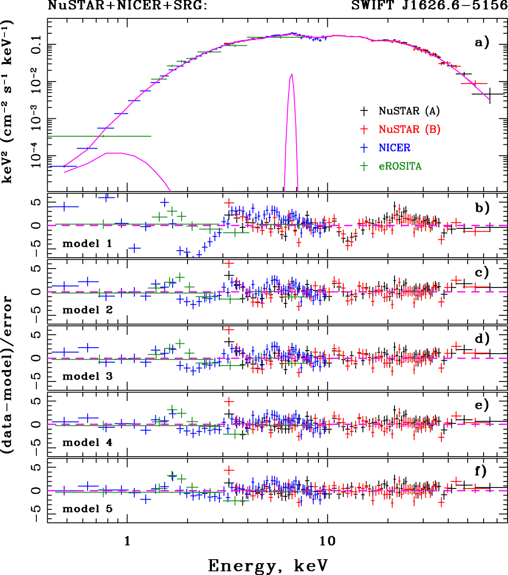
The spectrum of Swift J1626.6–5156 is typical for accreting XRPs (see, e.g., Nagase 1989; Filippova et al. 2005). It is characterized by an exponential cutoff at high energies (Figure 4), which can be explained in terms of the Comptonization processes in hot emission regions (see, e.g., Sunyaev & Titarchuk 1980; Meszaros & Nagel 1985; Titarchuk 1994). We modeled the broadband continuum spectrum with two commonly used phenomenological models: a power law with an exponential cutoff (cutoffpl in the xspec package, hereafter model1) and a thermal Comptonization model (comptt, hereafter model2). To take into account the uncertainty in calibrations of two modules of NuSTAR a cross-calibration constant C_modB was included in all spectral fits. Furthermore, two cross-calibration constants were added for NICER (C_NIC), and eROSITA (C_eRo) spectra, in order to compensate for some flux difference between the observations by these instruments (we assume that the spectrum shape does not change significantly). Depending on the continuum model, the inclusion of a soft blackbody component with the temperature of ∼0.1 keV improves the fit quality in the softer part of the spectrum (see also Iwakiri et al. 2021). We included in the fit a Gaussian function to model an emission of the neutral fluorescence iron line (Gauss), and the phabs component to take into account interstellar absorption. For both continua, an inclusion of two earlier reported absorption features around 10 and 20 keV was also necessary in order to obtain a meaningful fit (gabs). Results of the fit are presented in Figure 4(a) and Table. 1.

Zoom In Zoom Out Reset image size

Table 1. Best-fitting Results for the Swift J1626.6–5156 Averaged Spectrum for Five Models

	Model1	Model2	Model3	Model4	Model5
	pha×	pha×	pha×	pha×	pha×
	(bb+cutoff+ga)	(bb+comptt+ga)	(bb+comptt+ga)	(bb+comptt+ga)	(bb+comptt+ga)
	× 2 gabs	× 2 gabs	× 3 gabs	× 3 gabs	× 4 gabs
Parameter	Value	Value	Value	Value	Value
NH a	2.23 ± 0.02	0.77 ± 0.03	0.78 ± 0.03	0.61 ± 0.04	0.42 ± 0.05
kTBB, keV	0.08 ± 0.01	0.14 ± 0.01	0.14 ± 0.01	0.14 ± 0.01	0.13 ± 0.03
ABB b , ×103	654 ± 92	0.33 ± 0.06	0.34 ± 0.07	0.27 ± 0.03	0.03 ± 0.01
Γ	1.14 ± 0.01	⋯	⋯	⋯	⋯
Efold, keV	10.12 ± 0.12	⋯	⋯	⋯	−
Acut c , ×101	0.67 ± 0.01	⋯	⋯	⋯	⋯
T0, keV	⋯	0.89 ± 0.01	0.89 ± 0.01	0.99 ± 0.02	1.17 ± 0.08
Tp, keV	⋯	5.36 ± 0.04	5.32 ± 0.04	5.65 ± 0.07	5.74 ± 0.16
τp	⋯	4.22 ± 0.04	4.26 ± 0.04	3.83 ± 0.08	3.43 ± 0.25
Acomp, ×101	⋯	0.156 ± 0.002	0.157 ± 0.002	0.148 ± 0.002	0.157 ± 0.005
EFe, keV	6.38 ± 0.05	6.41 ± 0.03	6.41 ± 0.03	6.57 ± 0.03	6.59 ± 0.03
σFe, keV	0.61 ± 0.05	0.46 ± 0.03	0.46 ± 0.03	0.16 ± 0.05	0.13 ± 0.05
AFe d , ×103	0.64 ± 0.07	0.58 ± 0.05	0.58 ± 0.05	0.18 ± 0.03	0.16 ± 0.04
EWFe, eV	146	142	141	42	32
Ecyc1, keV	⋯	⋯	⋯	4.73 ± 0.05	4.82 ± 0.05
σcyc1, keV	⋯	⋯	⋯	0.58 ± 0.09	0.93 ± 0.09
τcyc1, keV	⋯	⋯	⋯	0.12 ± 0.03	0.47 ± 0.14
Ecyc2, keV	9.02 ± 0.06	8.94 ± 0.04	8.95 ± 0.05	8.78 ± 0.05	8.63 ± 0.06
σcyc2, keV	1.18 ± 0.08	0.77 ± 0.06	0.79 ± 0.06	1.00 ± 0.07	1.74 ± 0.20
τcyc2, keV	0.45 ± 0.03	0.21 ± 0.02	0.22 ± 0.02	0.38 ± 0.05	1.51 ± 0.56
Ecyc3, keV	⋯	⋯	12.96 ± 0.20	⋯	12.84 ± 0.11
σcyc3, keV	⋯	⋯	0.57 ± 0.26	⋯	0.97 ± 0.15
τcyc3, keV	⋯	⋯	0.06 ± 0.03	⋯	0.30 ± 0.11
Ecyc4, keV	17.00 ± 0.11	17.33 ± 0.10	17.37 ± 0.10	17.21 ± 0.10	17.09 ± 0.14
σcyc4, keV	1.06 ± 0.11	1.28 ± 0.11	1.45 ± 0.13	1.02 ± 0.11	1.65 ± 0.21
τcyc4, keV	0.37 ± 0.04	0.52 ± 0.05	0.63 ± 0.07	0.38 ± 0.04	0.82 ± 0.18
CmodB	1.064 ± 0.003	1.064 ± 0.003	1.064 ± 0.003	1.064 ± 0.003	1.064 ± 0.005
CNIC	0.917 ± 0.005	0.944 ± 0.005	0.944 ± 0.005	0.946 ± 0.005	0.948 ± 0.005
CeRo	0.772 ± 0.003	0.802 ± 0.003	0.802 ± 0.003	0.804 ± 0.003	0.805 ± 0.003
FX e , ×1010	5.5	5.5	5.5	5.5	5.5
χ2 (dof)	1604.0 (864)	1027.6 (863)	1015.4 (860)	930.3 (860)	906.9 (857)
goodness	100%	99%	99%	74%	54%
BIC	1657	1084	1080	995	981
Δ BIC	⋯	⋯	BICmodel2−	BICmodel2−	BICmodel4−
			BICmodel3 = 4	BICmodel4 = 89	BICmodel5 = 14

Notes. Here N_H is the column density, kT_BB is the blackbody temperature, Γ is the power-law photon index, E_fold is the folding energy of the cutoff power law. T₀, T_p, and τ_p are the seed photons temperature, the plasma temperature, and the plasma optical depth Comptonization model parameters, respectively. E_Fe, σ_Fe, and EW_Fe are the iron line energy, width, and equivalent width, respectively. E_cyc, σ_cyc, and τ_cyc are the energy, width, and optical depth of cyclotron lines, respectively.

^a Value of N_H is in units of 10²² atom cm⁻². ^b Normalization parameter calculated as L₃₉/D₁₀ ², where L₃₉ is the source luminosity in units of 10³⁹ erg s⁻¹ and D₁₀ is the distance to the source in units of 10 kpc. ^c Units are photons keV⁻¹ cm⁻² s⁻¹ at 1 keV. ^d Total photons cm⁻² s⁻¹ in the line. ^e Model flux in the 3–50 keV energy band in units of erg cm⁻² s⁻¹.

Download table as:  ASCIITypeset image

The quality of the fit, however, is not acceptable for both models. Although the reduced χ² value is around ∼1.2 for model2, an assessment of the fit quality using simulations (by means of a goodness command in Xspec) revealed an unsatisfactory quality of the fit (Table 1). Poor quality of the fit is also revealed by residuals that are observed around 5 and 13 keV (Figures 4(b), (c)). The quality of the fit could be improved by including additional absorption line features near 13 keV (model3, Figure 4(d)) or near 5 keV (model4, Figure 4(e)). We note, however, that including only one of the two lines does not result in a statistically acceptable fit. If we add only a 13 keV line, then neither fit-statistic nor Bayesian information criteria (appropriate for comparison of non-nested models) indicate significant improvement, and the goodness parameter remains at an unacceptable level. Adding only the 5 keV absorption feature leads to better approximation, and goodness parameter becomes closer to 50%. But only the inclusion of both lines (model5) dramatically improves the quality of the fit (Figure 4(f)) and makes it adequate both in terms of fit-statistics and Bayesian criteria, and as assessed with simulations using goodness command.

We finally conclude, therefore, that a statistically acceptable fit of the averaged spectrum can only be obtained if all four absorption features are included in the model. This, together with the fact that the centroid energies of these features appear to be harmonically spaced for a fundamental line energy at E ∼ 5 keV, strongly indicates that all four features have a physical origin.

On the other hand, also the best-fit discussed above has some issues. As can be seen in Table 1, the centroid of the iron line energy becomes significantly higher than the expected value of 6.4 keV in model4 and model5. We note that the equivalent width of this line is quite low, which might imply that the available statistics actually does not allow to significantly detect the line and constrain its parameters, so the increase of its apparent energy might be an artifact of the fit. Indeed, the shifted energy of the iron line appears in models with the addition of the soft absorption feature at E ∼ 5 keV (model4 and model5). Taking into account the fact that the both models contain an absorption line around E ∼ 9 keV, one can imagine the appearance of the emission-like feature in the region around 6–7 keV, especially if the centroid energies of these absorption features vary with the pulse phase. To investigate this issue in detail, we performed also the phase-resolved spectral analysis.

3.3. Pulse Phase-resolved Spectroscopy

It is well established that spectra of XRPs vary with the pulse phase. Parameters of the CRSFs are also know to change at such timescales (see, e.g., Burderi et al. 2000; Heindl et al. 2004; Kreykenbohm et al. 2004; Lutovinov et al. 2015, and references therein), and, in some cases, lines can only appear significantly at certain phase intervals (Molkov et al. 2019). Therefore, the pulse-phase-resolved spectroscopy can be considered as a tool for the study of the line properties, and ultimately for probing the geometry of the emission regions in the vicinity of the neutron star and its magnetic field structure. Here we focus on understanding whether the absorption features are detected at individual pulse phases in order to exclude the situation when the detection of the features in the averaged spectrum arises from the modeling of superimposed spectra variable across different pulse phases.

As a first step, we fitted phase-resolved NuSTAR and NICER spectra extracted from the 0.2 phase length intervals with the Comptonization model continuum modified by the interstellar absorption but without absorption or emission like features and soft blackbody component. Residuals of the fits relative to the absorption lines (Figure 5) are observed throughout the pulse, although the depth of the individual features appears to be variable and is most clearly seen at the phase interval 0.65–0.85.

Zoom In Zoom Out Reset image size

In the next step, we fitted these spectra, adding up to four absorption-like features. Unlike to the phase-averaged analysis, we did not include the soft blackbody component (fits are not sensitive to this, probably due to the lack of statistics in phase-resolved spectra) and the iron line. At all phases, the inclusion the two absorption features at E ∼ 5 keV and E ∼ 9 keV is necessary to obtain significant fits. For phases 0.05–0.25 and 0.25–0.45, these two components are actually sufficient. For phases 0.45–0.65 and 0.85–1.05 the inclusion of an additional absorption line at E ∼ 17 keV strongly improves the fit quality. In first case, the value of the χ² changes from 730 (650 dof) to 681 (647 dof), and in the second, from 671 (579 dof) to 644 (576 dof). In terms of Bayesian criteria, we obtain ΔBIC = 41 and ΔBIC = 19 for the first and the second cases, respectively, which implies (since both values are >10) that the strength of statement that the model with three lines is better than with two lines is "Very strong." Finally, to achieve an acceptable fit for the spectrum at phase 0.65–0.85, all four absorption lines have to be included. More specifically, the χ² value changes from 796 (660 dof) to 704 (657 dof) after adding the line at ∼17 keV, and reduces to 630 (564 dof) after a fourth absorption line feature at ∼13 keV is included (see Figure 6). Bayesian information criterion decreases on 83 and 65, respectively. Results of the approximation of the phase-resolved spectra are summarized in Table 2.

Zoom In Zoom Out Reset image size

Table 2. Best Parameters of the Swift J1626.6–5156 Phase-resolved Spectra Fitting with the Comptonization Model Modified by Interstellar Absorption and with Inclusion of up to Four Cyclotron-line Absorption Features

Phase	0.05–0.25	0.25–0.45	0.45–0.65	0.65–0.85	0.85–1.05
Parameter	Value	Value	Value	Value	Value
NH	0.37 ± 0.02	0.44 ± 0.03	0.43 ± 0.02	0.42 ± 0.02	0.28 ± 0.03
T0, keV	1.14 ± 0.03	1.10 ± 0.03	1.17 ± 0.03	1.18 ± 0.03	1.21 ± 0.08
Tp, keV	6.38 ± 0.37	6.25 ± 0.25	6.24 ± 0.28	6.06 ± 0.21	6.57 ± 0.58
τp	2.86 ± 0.23	3.19 ± 0.20	3.13 ± 0.21	3.38 ± 0.19	2.85 ± 0.40
Acomp × 101	0.114 ± 0.002	0.142 ± 0.005	0.180 ± 0.007	0.191 ± 0.006	0.103 ± 0.007
Ecyc1, keV	4.88 ± 0.06	4.99 ± 0.05	5.00 ± 0.06	4.90 ± 0.06	4.61 ± 0.08
σcyc1, keV	0.75 ± 0.10	0.72 ± 0.08	0.95 ± 0.07	1.02 ± 0.10	0.87 ± 0.11
τcyc1, keV	0.30 ± 0.08	0.33 ± 0.08	0.53 ± 0.08	0.47 ± 0.12	0.42 ± 0.12
Ecyc2, keV	8.79 ± 0.08	9.22 ± 0.12	8.54 ± 0.05	8.39 ± 0.04	9.02 ± 0.16
σcyc2, keV	1.46 ± 0.16	1.73 ± 0.19	1.41 ± 0.09	1.09 ± 0.09	2.19 ± 0.42
τcyc2, keV	0.93 ± 0.21	0.98 ± 0.24	1.20 ± 0.15	0.91 ± 0.17	1.64 ± 0.90
Ecyc3, keV	⋯	⋯	⋯	12.56 ± 0.08	⋯
σcyc3, keV	⋯	⋯	⋯	0.64 ± 0.13	⋯
τcyc3, keV	⋯	⋯	⋯	0.28 ± 0.07	⋯
Ecyc4, keV	⋯	⋯	17.55 ± 0.22	16.86 ± 0.09	16.90 ± 0.26
σcyc4, keV	⋯	⋯	1.34 ± 0.26	0.84 ± 0.11	1.23 ± 0.35
τcyc4, keV	⋯	⋯	0.56 ± 0.13	0.58 ± 0.08	0.54 ± 0.21
CmodB	1.063 ± 0.006	1.067 ± 0.006	1.075 ± 0.005	1.075 ± 0.005	1.074 ± 0.007
CNIC	0.933 ± 0.011	0.960 ± 0.011	0.979 ± 0.010	0.976 ± 0.010	0.917 ± 0.012
FX × 1010	3.6	4.5	5.7	6.1	3.1
χ2 (dof)	601.3 (592)	745.6 (626)	681.2 (647)	630.1 (654)	643.8 (576)

Note. See notes to Table 1.

Download table as:  ASCIITypeset image

Thus, we have confirmed presence of all four absorption features in the phase-resolved spectra as well. However, not all lines are detected in all phase bins. We also note that their energies vary slightly with the pulse phase. In addition, we note that to describe the phase-resolved spectra, it is not necessary to include a component for the iron line.

Most of the known cyclotron-line sources exhibit either only the fundamental CRSF or the fundamental one and its first harmonic. This is likely a selection effect associated with the difficulty of detecting such features at higher energies. In fact, most accreting pulsars are strongly magnetized with fundamental line energies typically above the cutoff energy at around 20 keV (see e.g., Staubert et al. 2019 for a recent review). The detection of the first, and certainly of the second, harmonics is challenging due to the lack of photons well above the cutoff.

In our analysis, we not only confirm the CRSFs at 8.6 and 17.1 keV in the spectrum of Swift J1626.6–5156 already reported in literature, but also discover two additional features around ∼4.9 keV and ∼13 keV. We conclude, therefore, that four CRSFs characterize the spectrum of Swift J1626.6–5156, with the fundamental line at E ∼ 4.9 keV, and that the other three features are harmonics. This implies that Swift J1626.6–5156 has the lowest confirmed magnetic field among all XRPs, and is only second to 4U 0115+63 (Santangelo et al. 1999) by the total number of observed cyclotron lines.

In the case of Swift J1626.6–5156, the detection of four lines is only possible due to the low energy of the fundamental one. The strength of the neutron star magnetic field is thus estimated to be B ∼ 4.1(1+z) × 10¹¹ G. The only other XRP with a comparable field is the peculiar "bursting pulsar" GRO J1744–28 (D'Aì et al. 2015; Doroshenko et al. 2015). Our result is rather unexpected and it is interesting to compare the magnetic field strength estimated through the CRSF with other indirect estimates.

First, as previously mentioned, we note that the source continues to accrete in quiescence (Tsygankov et al. 2017) down to a bolometric luminosity of ≃5.9 × 10³³ d₁₀ ² erg s⁻¹ (here we recalculated the lowest observed luminosity in the 0.5–10 keV energy band to the bolometric one based on our knowledge of the source broadband spectrum and d₁₀ is distance to the source scaled to 10 kpc). This is consistent with the observed eROSITA flux and the source flux variability at low luminosities as illustrated by Figure 7. If the accretion continues, then the lowest luminosity value must have been higher than the limiting luminosity for the transition to the propeller regime (Tsygankov et al. 2016):

$$\begin{eqnarray*}&&{L}_{\mathrm{lim}}=4\times {10}^{37}{k}^{7/2}{B}_{12}^{2}{P}^{-7/3}{M}_{1.4}^{-2/3}{R}_{6}^{5}\leqslant {L}_{10}{d}_{10}^{2}.\end{eqnarray*}$$

Here k is a factor relating to the size of the magnetosphere for a given accretion configuration to the Alfvén radius, B₁₂ is the magnetic field in units of 10¹² G, and L₁₀ is a lowest measure bolometric flux of the source calculated in assumption of 10 kpc distance. Assuming canonical neutron star parameters of M = 1.4M_☉, R = 10⁶ cm and k = 0.5, the measured source minimal luminosity L₁₀ = 5.9 × 10³³ erg s⁻¹, and the spin period of 15.4 s, one obtains the magnetic field value B₁₂ ≤ 1 × d₁₀. Considering the limits on distance from Gaia EDR3 of 5.8–12 kpc (Bailer-Jones et al. 2021), B₁₂ ≤ (0.58–1.2) × 10¹² G. Although formally consistent with interpretation of either 4.9 keV and 9 keV lines as fundamental, the line at 9 keV is already at the edge of the allowed distance range and inconsistent with the best photogeometric Gaia estimate of 6.6 kpc. We conclude, therefore, that also observed properties of Swift J1626.6–5156 in quiescence favor the low field implied by ∼4.9 keV fundamental cyclotron-line energy.

Zoom In Zoom Out Reset image size

This makes Swift J1626.6–5156 the weakest magnetized classical XRP among all cyclotron-line sources, and might have relevant consequences for the science program of upcoming X-ray polarimeters such as the Imaging X-ray Polarimetry Explorer (IXPE; Weisskopf et al. 2016), and the polarization focusing array on board the enhanced X-ray Timing and Polarimetry (eXTP) mission (Zhang et al. 2016; Santangelo et al. 2019). Indeed, those instruments operate in the soft X-ray band where the emission of XRPs is expected to be strongly polarized due to the birefringence induced by a Compton scattering in the strong magnetic field (Meszaros et al. 1988) for ordinary and extraordinary mode photons. The cross-sections for photons with both modes become comparable around the cyclotron resonance energy, which makes this energy extremely interesting. For the vast majority of XRPs the cyclotron resonance energy lies outside of the operational range of the gas pixel detectors used in IXPE/eXTP polarimeters. The only exceptions are Swift J1626.6–5156 and GRO J1744–28. However, GRO J1744–28 has a very low outburst duty cycle, and thus it is unlikely that it will be observed. On the other hand, Swift J1626.6–5156 appears to be regularly detectable by all sky monitors and wide field X-ray instruments, and thus is the ideal target for the forthcoming X-ray polarimeters, especially if it undergoes another giant outburst.

We thank the NuSTAR team for the help with organizing prompt observation. This work was financially supported by the Russian Science Foundation (grant 19-12-00423).