


Abstract
We search for an isotropic stochastic gravitational-wave background (GWB) in the 12.5 yr pulsar-timing data set collected by the North American Nanohertz Observatory for Gravitational Waves. Our analysis finds strong evidence of a stochastic process, modeled as a power law, with common amplitude and spectral slope across pulsars. Under our fiducial model, the Bayesian posterior of the amplitude for an f−2/3 power-law spectrum, expressed as the characteristic GW strain, has median 1.92 × 10⁻¹⁵ and 5%–95% quantiles of 1.37–2.67 × 10⁻¹⁵ at a reference frequency of  the Bayes factor in favor of the common-spectrum process versus independent red-noise processes in each pulsar exceeds 10,000. However, we find no statistically significant evidence that this process has quadrupolar spatial correlations, which we would consider necessary to claim a GWB detection consistent with general relativity. We find that the process has neither monopolar nor dipolar correlations, which may arise from, for example, reference clock or solar system ephemeris systematics, respectively. The amplitude posterior has significant support above previously reported upper limits; we explain this in terms of the Bayesian priors assumed for intrinsic pulsar red noise. We examine potential implications for the supermassive black hole binary population under the hypothesis that the signal is indeed astrophysical in nature.
Export citation and abstract BibTeX RIS
1. Introduction
Pulsar-timing arrays (PTAs; Sazhin 1978; Detweiler 1979; Foster & Backer 1990) seek to detect very-low-frequency (∼1–100 nHz) gravitational waves (GWs) by monitoring the spatially correlated fluctuations induced by the waves on the times of arrival of radio pulses from millisecond pulsars (MSPs). The dominant source of gravitational radiation in this band is expected to be the stochastic background generated by a cosmic population of supermassive black hole binaries (SMBHBs; Sesana et al. 2004; Burke-Spolaor et al. 2019). Other more speculative stochastic GW sources in the nanohertz frequency range include cosmic strings (Siemens et al. 2007; Blanco-Pillado et al. 2018), phase transitions (Caprini et al. 2010; Kobakhidze et al. 2017), and a primordial GW background (GWB) produced by quantum fluctuations of the gravitational field in the early universe, amplified by inflation (Grishchuk 1975; Lasky et al. 2016).
The North American Nanohertz Observatory for Gravitational Waves (NANOGrav; Ransom et al. 2019) has been acquiring pulsar-timing data since 2004. NANOGrav is one of three major PTAs along with the European Pulsar Timing Array (EPTA; Desvignes et al. 2016) and the Parkes Pulsar Timing Array (PPTA; Kerr et al. 2020). Additionally, there are growing PTA efforts in India (Joshi et al. 2018) and China (Lee 2016), as well as some telescope-centered timing programs (Bailes et al. 2016; Ng 2018). In concert, these collaborations support the International Pulsar Timing Array (IPTA; Perera et al. 2019). Over the last decade, PTAs have produced increasingly sensitive data sets, as seen in the steady march of declining upper limits on the stochastic GWB (van Haasteren et al. 2011; Demorest et al. 2013; Shannon et al. 2013; Lentati et al. 2015; Shannon et al. 2015; Arzoumanian et al. 2016, 2018a; Verbiest et al. 2016). It was widely expected that the first inklings of a GWB would manifest in the stagnation of improvement in upper limits, followed by the emergence of a spatially uncorrelated common-spectrum red process in all pulsars, and culminate in the detection of interpulsar spatial correlations with the quadrupolar signature described by Hellings & Downs (1983). In practice, it appears that early indications of a signal may have been obscured by systematic effects due to incomplete knowledge of the assumed position of the solar system barycenter (Vallisneri et al. 2020).
In this article, we present our analysis of NANOGrav's newest "12.5 yr" data set (Alam et al. 2021a, hereafter NG12). We find a strong preference for a stochastic common-spectrum process, modeled as a power law, in the timing behaviors of all pulsars in the data set. Building on the statistical-inference framework put in place during our GW study of the 11 yr data set (Arzoumanian et al. 2018a, hereafter NG11gwb), we report Bayes factors from extensive model comparisons. We find the log10 Bayes factor for a spatially uncorrelated common-spectrum process versus independent red-noise processes in each pulsar to range from 2.7 to 4.5, depending on which solar system ephemeris (SSE) modeling scheme we employ. We model a spatially uncorrelated common-spectrum process to have the same power spectral density across all pulsars in the data set, but with independent realizations in the specific timing behavior of each pulsar. The evidence is only slightly higher for a common-spectrum process with quadrupolar correlations, with a log10 Bayes factor against a spatially uncorrelated common-spectrum process ranging from 0.37 to 0.64, again depending on SSE modeling. Correspondingly, the Bayesian–frequentist hybrid optimal-statistic analysis (Anholm et al. 2009; Demorest et al. 2013; Chamberlin et al. 2015; Vigeland et al. 2018), which measures interpulsar correlated power only, is unable to distinguish between different spatially correlated processes. Thus, lacking definitive evidence of quadrupolar spatial correlations, the analysis of this data set must be considered inconclusive with regard to GW detection.
With an eye toward searches in future, more informative data sets, we perform a suite of statistical tests on the robustness of our findings. Focusing first on the stochastic common-spectrum process, we examine the contribution of each pulsar to the overall Bayes factor with a dropout analysis (Aggarwal et al. 2019; S. Vigeland et al. 2020, in preparation) and find broad support among the pulsars in the data set. Moving on to spatial correlations, we build null background distributions for the correlation statistics by applying random phase shifts and sky scrambles to our data (Cornish & Sampson 2016; Taylor et al. 2017a) and find that the no-correlations hypothesis is rejected only mildly, with p values ∼5% (i.e., 2σ).
The posterior on the amplitude of the common-spectrum process,  , modeled with an f−2/3 power-law spectrum, has a median of 1.9 × 10⁻¹⁵, with 5%–95% quantiles of 1.4–2.7 × 10⁻¹⁵ at a reference frequency of
  , based on a log-uniform prior and using the latest JPL SSE (DE438, Folkner & Park 2018), which we take as our fiducial model in this paper. This refined version of the SSE incorporates data from the NASA orbiter Juno
45
and claims a Jupiter orbit accuracy a factor of 4 better than previous SSEs, which is promising given that our previous analysis showed that errors in Jupiter's orbit dominated the SSE-induced GWB systematics (Vallisneri et al. 2020).
, based on a log-uniform prior and using the latest JPL SSE (DE438, Folkner & Park 2018), which we take as our fiducial model in this paper. This refined version of the SSE incorporates data from the NASA orbiter Juno
45
and claims a Jupiter orbit accuracy a factor of 4 better than previous SSEs, which is promising given that our previous analysis showed that errors in Jupiter's orbit dominated the SSE-induced GWB systematics (Vallisneri et al. 2020).
The fact that the median value of  is higher than the 95% upper limit reported for the 11 yr data set,
  (NG11gwb), requires explanation. While many factors contribute to this discrepancy, simulations show that the standard PTA data model (and most crucially, the uniform priors on the amplitude of pulsar-intrinsic red-noise processes) can often yield Bayesian upper limits lower than the true GWB level by shifting GWB power to pulsar red noise (Hazboun et al. 2020a). Once all factors are taken into account, the data sets can be reconciled. However, this accounting suggests that the astrophysical interpretation of past Bayesian upper limits from PTAs may have been overstated. Indeed, it is worth noting that while the source of the common-spectrum process in this data set remains unconfirmed, the posterior on
  is compatible with many models for the GWB that had previously been deemed in tension with PTA analyses.
This paper is laid out as follows: Section 2 describes the 12.5 yr data set. Our data model is presented in Section 3. In Section 4, we report on our search for a common-spectrum process in the data set and present the results from our extensive exploration for interpulsar correlations. Section 5 contains a suite of statistical checks on the significance of our detection metrics. In Section 6, we discuss the amplitude of the recovered process, addressing both the discrepancies with previous published upper limits and the potential implications for the SMBHB population, and we conclude with our expectations for future searches.
2. The 12.5 yr Data Set
The NANOGrav 12.5 yr data set has been released using two separate and independent analyses. The narrowband analysis, consisting of the time-of-arrival (TOA) data and pulsar-timing models presented in NG12, is very similar in its form and construction to our previous data sets in which many TOAs were calculated within narrow radio-frequency bands for data collected simultaneously across a wide bandwidth. A separate "wideband" analysis (Alam et al. 2021b) was also performed in which a single TOA is extracted from broadband observations. Both versions of the data set are publicly available online. 46 The data set consists of observations of 47 MSPs made between 2004 July and 2017 June. This is the fourth public NANOGrav data set and adds two MSPs and 1.5 yr of observations to the previously released 11 yr data set (NG11). Only pulsars with a timing baseline greater than 3 yr are used in our GW analyses (Arzoumanian et al. 2016, hereafter NG9gwb), and thus all results in this paper are based on the 45 pulsars that meet that criteria. This is a significant increase from the analyses in NG11gwb, which used 34 pulsars, and the analyses in NG9gwb, which used 18. Additionally, it is crucial to note that the 12.5 yr data set is more than just an extension of the 11 yr data set—changes to the data-processing pipeline, discussed below, have improved the entire span of the data. In the following section, we briefly summarize the instruments, observations, and data reduction process for the 12.5 yr data set. A more detailed discussion of the data set can be found in NG12.
2.1. Observations
We used the 305 m Arecibo Observatory (Arecibo or AO) and the 100 m Green Bank Telescope (GBT) to observe the pulsars. Arecibo observed all sources that lie within its decl. range (0° < δ < +39°), while GBT observed those sources that lie outside of Arecibo's decl. range, plus PSRs J1713+0747 and B1937+21. Most sources were observed approximately once per month. Six pulsars were observed weekly as part of a high-cadence observing campaign, which began at the GBT in 2013 and at AO in 2015 with the goal of improving our sensitivity to individual GW sources (Burt et al. 2011; Christy et al. 2014): PSRs J0030+0451, J1640+2224, J1713+0747, J1909−3744, J2043+1711, and J2317+1439.
Early observations were recorded using the ASP and GASP systems at Arecibo and GBT, respectively, which sampled bandwidths of 64 MHz (Demorest 2007). Between 2010 and 2012, we transitioned to wideband systems (PUPPI at Arecibo and GUPPI at GBT) that can process up to 800 MHz bandwidths (DuPlain et al. 2008; Ford et al. 2010). At most observing epochs, the pulsars were observed with two different wideband receivers covering different frequency ranges in order to achieve good sensitivity in the measurement of pulse dispersion due to the interstellar medium. At Arecibo, the pulsars were observed using the 1.4 GHz receiver plus either the 430 MHz receiver or 2.1 GHz receiver, depending on the pulsar's spectral index and timing characteristics. (Early observations of one pulsar also used the 327 MHz receiver.) At GBT, the monthly observations used the 820 MHz and 1.4 GHz receivers. However, these two separate frequency ranges were not observed simultaneously; instead, the observations were separated by a few days. The weekly observations at GBT used only the 1.4 GHz receiver.
2.2. Processing and Time-of-arrival Data
Most of the procedures used to reduce the data, generate the TOAs, and clean the data set were similar to those used to generate previous NANOGrav data sets (NG9, NG11); however, several new steps were added. We improved the data reduction pipeline by removing low-amplitude artifact images from the profile data that are caused by small mismatches in the gains and timing of the interleaved analog-to-digital converters in the backends. We also excised radio-frequency interference (RFI) from the calibration files as well as the data files.
We used the same procedures as in NG9 and NG11 to generate the TOAs from the profile data. As we have done in previous data sets, we cleaned the TOAs by removing RFI, low signal-to-noise TOAs (NG9), and outliers (NG11). Compared to previous data sets, we reorganized and systematized the TOA cleaning and timing-model parameter selection processes to improve consistency of processing across all pulsars. We also performed a new test where observing epochs were removed one by one to determine whether removing a particular epoch significantly changed the timing model. This is essentially an outlier analysis for observing epochs rather than individual TOAs.
2.3. Timing Models and Noise Analysis
For each pulsar, the cleaned TOAs were fit to a timing model that described the pulsar's spin period and spin period derivative, sky location, proper motion, and parallax. For binary pulsars, the timing model also included five Keplerian binary parameters and additional post-Keplerian parameters if they improved the timing fit as determined by an F test. We modeled variations in the pulse dispersion as a piecewise constant through the inclusion of DMX parameters (NG9; Jones et al. 2017). The timing-model fits were primarily performed using the tempo timing software, and the software packages tempo2 and pint were used to check for consistency. The timing-model fits were done using the TT(BIPM2017) timescale and the JPL SSE model DE436 (Folkner & Park 2016). The latest JPL SSE (DE438; Folkner & Park 2018), which we take as our fiducial model for the analyses in this paper, was not available when TOA processing was being done. However, this does not affect the results presented later, as the corresponding changes in the timing parameters are well within their linear range, which is marginalized away in the analysis (NG9, NG9gwb).
We modeled noise in the pulsars' residuals with three white-noise components plus a red-noise component. The white-noise components are EQUAD, which adds white noise in quadrature; ECORR, which describes white noise that is correlated within the same observing epoch but uncorrelated between different observing epochs; and EFAC, which scales the total template-fitting TOA uncertainty after the inclusion of the previous two white-noise terms. For all of these components, we used separate parameters for every combination of pulsar, backend, and receiver.
Many processes can produce red noise in pulsar residuals. The stochastic GWB appears in the residuals as red noise; however, it appears specifically correlated between different pulsars (Hellings & Downs 1983). Other astrophysical sources of red noise include spin noise, pulse profile changes, and imperfectly modeled dispersion-measure variations (Cordes 2013; Jones et al. 2017; Lam et al. 2017). These red-noise sources are unique to a given pulsar. There are also potential terrestrial sources of red noise, including clock errors and ephemeris errors (Tiburzi et al. 2016), which are correlated differently than the GWB. We model the intrinsic red noise of each pulsar as a power law, similar to the GWB (see Section 3.1).
The changes to the data-processing procedure described above significantly improved the quality of the data. In order to quantify the effect of these changes, we produced an "11 yr slice" data set by truncating the 12.5 yr data set at the MJD corresponding to the last observation in the 11 yr data set and compared the results of a full noise analysis of this data set to those for the 11 yr data set. As discussed in NG12, we found a reduction in the amount of white noise in the 11 yr slice compared to the 11 yr data set. However, we also found that the red noise changed for many pulsars. Specifically, there is a slight preference for a steeper spectral index across most of the pulsars, indicating that for some pulsars, the reduction in white noise produced an increased sensitivity to low-frequency red-noise processes, like the GWB.
3. Data Model
The statistical framework for the characterization of noise processes and GW signals in pulsar-timing data is well documented (see e.g., NG9gwb; NG11gwb). In this section, we give a concise description of our probabilistic model of the 12.5 yr data set, focusing on the differences from earlier studies. The model attempts to represent every known deterministic and stochastic source of timing residuals that could be interpreted as GWs: it extends the individual timing models of the pulsars (discussed in Section 2.3) by adding common-spectrum processes with specific correlation structures between pulsars. In Section 3.1, we define our spectral models of time-correlated (red) processes, which include pulsar-intrinsic red noise and the GWB; in Section 3.2, we list the combinations of time-correlated processes included in our Bayesian model-comparison trials; and in Section 3.3, we discuss our prescriptions for the SSE. Our Bayesian and frequentist techniques of choice will be described alongside our results in Sections 4 and 5, with more technical details in Appendices B and C.
3.1. Models of Time-correlated Processes
The principal results of this paper are referred to a fiducial power-law spectrum of the characteristic GW strain:

with α = −2/3 for a population of inspiraling SMBHBs in circular orbits whose evolution is dominated by GW emission (Phinney 2001). We performed our analysis in terms of the timing-residual cross-power spectral density,

where γ = 3 − 2α (so the fiducial SMBHB α = −2/3 corresponds to γ = 13/3) and where Γab is the overlap reduction function (ORF), which describes average correlations between pulsars a and b in the array as a function of the angle between them. For an isotropic GWB, the ORF is given by Hellings & Downs (1983), and we refer to it casually as "quadrupolar" or "HD" correlations.
Other spatially correlated effects present with different ORFs. Systematic errors in the SSE have a dipolar ORF,  , where ζab
represents the angle between pulsars a and b, while errors in the timescale (the "clock") have a monopolar ORF, Γab
= 1. Pulsar-intrinsic red noise is also modeled as a power law; however, in that case, there is no ORF. The AGWB in Equation (2) is replaced with Ared, and γ with γred. There is a separate (Ared, γred) pair for each pulsar in the array.
, where ζab
represents the angle between pulsars a and b, while errors in the timescale (the "clock") have a monopolar ORF, Γab
= 1. Pulsar-intrinsic red noise is also modeled as a power law; however, in that case, there is no ORF. The AGWB in Equation (2) is replaced with Ared, and γ with γred. There is a separate (Ared, γred) pair for each pulsar in the array.
As in NG9gwb and NG11gwb, we implemented stationary Gaussian processes with a power-law spectrum in rank-reduced fashion by approximating them as a sum over a sine–cosine Fourier basis with frequencies k/T and prior (weight) covariance  , where T is the span between the minimum and maximum TOAs in the array (van Haasteren & Vallisneri 2014). We use the same basis vectors to model all red noise in the array, both pulsar-intrinsic noise and global signals, like the GWB. Using a common set of vectors helps the sampling and reduces the likelihood computation time. In previous work, the number of basis vectors was chosen to be large enough (with k = 1, ..., 30) that inference results (specifically the Bayesian upper limit) for a common-spectrum signal became insensitive to adding more components. However, doing so has the disadvantage of potentially coupling white noise to the highest-frequency components of the red-noise process, thus biasing the recovery of the putative GWB, which is strongest in the lowest frequency bins.
For this paper, we revisit the issue and set the number of frequency components used to model common-spectrum signals to five, on the basis of theoretical arguments backed by a preliminary analysis of the data set. We begin with the former. By computing a strain-spectrum sensitivity curve for the 12.5 yr data set using the hasasia tool (Hazboun et al. 2019) and obtaining the signal-to-noise ratio (S/N) of a γ = 13/3 power-law GWB, we observed that the five lowest frequency bins contribute 99.98% of the S/N, with the majority coming from the first bin. We also injected a γ = 13/3 power-law GWB into the 11 yr data set (NG11), and measured the response of each frequency using a 30-frequency free-spectrum model, in which we allowed the variance of each sine–cosine pair in the red-noise Fourier basis to vary independently. We observed that the lowest few frequencies are the first to respond as we raised the GWB amplitude from undetectable to detectable levels (see Figure 14 in Appendix A). The details of this injection analysis are described in Appendix A.
Moving on to empirical arguments, in Figure 1 we plot the power-spectrum estimates for a spatially uncorrelated common-spectrum process in the 12.5 yr data set, as computed for the following: a free-spectrum model (gray violin plots); variable-γ power-law models (Equation (2) with  and
and  ) with 5 and 30 frequency components (dashed lines, showing maximum a posteriori values, as well as 1σ/2σ posterior contours); and a broken power-law model (solid lines), given by

where γ and δ are the slopes at frequencies lower and higher than fbend, respectively, and κ controls the smoothness of the transition. In this paper, we set δ = 0 to appropriately capture the white noise coupled at higher frequencies and κ = 0.1, which is small enough to contain the transition between slopes to within an individual frequency bin. Both the free spectrum and the broken power law capture a steep red process at the lowest frequencies, in accordance with expectations for a GWB, which is accompanied by a flatter "forest" at higher frequencies. The 30-frequency power law is impacted by power at high frequencies (where we do not expect any detectable contributions from a GWB) and adopts a low spectral index that does not capture the full power in the lowest frequencies. By contrast, the five-frequency power law agrees with the free spectrum and broken power law in recovering a steep-spectral process.

Figure 1. Posteriors for a common-spectrum process in NG12, as recovered with four models: free spectrum (gray violin plots in left panel), broken power law (solid blue lines and contours), 5-frequency power law (dashed orange lines and contours), and 30-frequency power law (dotted–dashed green lines and contours). In the left panel, the violin plots show marginalized posteriors of the equivalent amplitude of the sine–cosine Fourier pair (i.e.,  , in units of seconds) at the frequencies on the horizontal axis; the lines show the mean reconstructed power laws in the left panel, and the 1σ (thicker) and 2σ posterior contours for the amplitude and spectral slope in the right panel. In the left panel, the shaded regions trace ±1σ ranges for the common-spectrum process power as a function of frequency, as implied by the Bayesian posteriors for the power-law parameters. The dotted vertical line in the left panel sits at
  , where PTA sensitivity is reduced by the fitting of timing-model parameters; the corresponding free-spectrum amplitude posterior is unconstrained. The dashed vertical line in the right panel sits at γ = 13/3, the expected value for a GWB produced by a population of inspiraling SMBHBs. For both the broken power-law and 5-frequency power-law models, the amplitude (
 ) posterior shown on the right is extrapolated from the lowest frequencies to the reference frequency
  . We observe that the slope and amplitude of the 30-frequency power law are driven by higher-frequency noise, whereas the 5-frequency power law recovers the low-frequency GWB-like slope of the free spectrum and broken power law.
Download figure:
Standard image High-resolution imageThe problem of pulsar-intrinsic excess noise leaking into the common-spectrum process at high frequencies has already been discussed for the 9 and 11 yr NANOGrav data sets (Aggarwal et al. 2019, 2020; Hazboun et al. 2020b), and we are addressing it through the creation of individually adapted noise models for each pulsar (J. Simon et al. 2020, in preparation). For this paper, we find a simpler solution by limiting all common-spectrum models to the five lowest frequencies. By contrast, we used 30 frequency components for all rank-reduced power-law models of pulsar-intrinsic red noise, 47 which is consistent with what is used in individual pulsar noise analyses and in the creation of the data set.
3.2. Models of Spatially Correlated Processes
We analyzed the 12.5 yr data set using a hierarchy of data models, which are compared in Bayesian fashion by evaluating the ratios of their evidence. All models include the same basic block for each pulsar, consisting of measurement noise, timing-model errors, pulsar-intrinsic white noise, and pulsar-intrinsic red noise described by a 30-frequency variable-γ power law, but they differ by the presence of one or two red-noise processes that appear in all pulsars with the same spectrum. As in previous work (NG9gwb; NG11gwb), we fixed all pulsar-intrinsic white-noise parameters to their maximum in the posterior probability distribution recovered from single-pulsar noise studies for computational efficiency.
The models are listed in Table 1, which also reports their labels as used in NG11gwb. The most basic variant (model 1 in NG11gwb) includes measurement noise and pulsar-intrinsic processes alone.
Table 1. Data Models
| NG11gwb Labels | 1 | 2A | 2B | 2D | 3A | (New) | 3B | 3D |
|---|---|---|---|---|---|---|---|---|
| Spatial Correlations | Single Common-spectrum Process | Two Common-spectrum Processes | ||||||
| Uncorrelated |

|

| ||||||
| Dipole |

|

| ||||||
| Monopole |

|

| ||||||
| HD |

|

|

|

| ||||
| Pulsar-intrinsic red-noise |

|

|

|

|

|

|

|

|
Note. The data models analyzed in this paper are organized by the presence of spatially correlated common-spectrum noise processes. Model names are added for a direct comparison to the naming scheme employed in NG11gwb.
Download table as: ASCIITypeset image
The next group of four models includes a single common-spectrum red-noise process. The first among them (model 2A of NG11gwb) features a GWB-like red-noise process with common spectrum, but without HD correlations. Because we expect the correlations to be much harder to detect than the diagonal Saa terms in Equation (2), due to the values of the HD ORF (Γab ) being less than or equal to 0.5, and because the corresponding likelihood, which does not include any correlations, is very computationally efficient, this model has been the workhorse of PTA searches. However, the positive identification of a GWB will require evidence of a common-spectrum process with HD correlations, which also belongs to this group (model 3A of NG11gwb). The group is rounded out by common-spectrum processes with dipolar and monopolar spatial correlations, which may represent SSE and clock anomalies. For a convincing GWB detection, we expect the data to favor HD correlations strongly over dipolar, monopolar, or no spatial correlations.
The last group includes an additional common-spectrum red-noise process on top of the GWB-like common-spectrum HD-correlated process. The second process is taken to have either no spatial correlations, dipolar correlations, or monopolar correlations.
3.3. Solar System Ephemeris
In the course of the GWB analysis of NANOGrav's 11 yr data set (NG11gwb), we determined that GW statistics were surprisingly sensitive to the choice of SSE, and we developed a statistical treatment of SSE uncertainties (BayesEphem; Vallisneri et al. 2020), designed to harmonize GW results for SSEs ranging from JPL's DE421 (published in 2009 and based on data up to 2007) to DE436 (published in 2016, and based on data up to 2015).
This was a rather conservative choice: it would be reasonable to expect that more recent SSEs, based on larger data sets and on more sophisticated data reduction, would be more accurate—an expectation backed by the (somewhat fragmentary) error estimates offered by SSE compilers. However, our analysis showed that errors in Jupiter's orbit (which create an apparent motion of the solar system barycenter and therefore a spurious Rømer delay) dominate the GWB systematics and that Jupiter's orbit has been adjusted across DE421–DE436 by amounts (≲50 km) comparable to or larger than the stated uncertainties. Thus, we decided to err on the side of caution, with the understanding that the Bayesian marginalization over SSE uncertainties would subtract power from the putative GWB process, as confirmed by simulations (Vallisneri et al. 2020).
Luckily, these circumstances have since changed. Jupiter's orbit is being refined with data from the NASA orbiter Juno: the latest JPL SSE (DE438, Folkner & Park 2018) fits the range and VLBI measurements from six perijoves and claims orbit accuracy a factor of 4 better than previous SSEs (i.e., ≲10 km). In addition, the longer time span of the 12.5 yr data set (NG12) reduces the degeneracy between a GWB and Jupiter's orbit (Vallisneri et al. 2020). Accordingly, we adopt DE438 as the fiducial SSE for the results reported in this paper. For completeness and verification, we also report statistics obtained with BayesEphem, adopting the same treatment of NG11gwb; and with the SSE INPOP19a (Fienga et al. 2019), which incorporates range data from nine Juno perijoves.
The DE438 and INPOP19a Jupiter orbit estimates are not entirely compatible, because the underlying data sets do not overlap completely and are weighted differently; nevertheless, the orbits differ in ways that affect GWB results only slightly, which further increases our confidence in DE438. In our analysis, we used DE438 and INPOP19a without uncertainty corrections: while it is technically straightforward to constrain BayesEphem using the orbital-element covariance matrices provided by the SSE authors, the resulting orbital perturbations are so small that GW results are barely affected (Vallisneri et al. 2020).
4. Gravitational-wave Background Estimates
Our Bayesian analysis of the 12.5 yr data set shows definitive evidence for the presence of a time-correlated stochastic process with a common amplitude ACP and a common spectral index γCP across all pulsars. Given this finding, we do not quote an upper limit on a GWB amplitude as in NG9gwb and NG11gwb, but rather report the median value and 90% credible interval of ACP, as well as the log10 Bayes factor for a common-spectrum process versus pulsar-intrinsic red noise only. Further details of our Bayesian methodology can be found in Appendix B. In addition, we characterize the evidence for HD correlations, which we take as the crucial marker of GWB detection, by obtaining the Bayes factors between the models of Table 1.
Our results are presented in Section 4.1 and summarized in Figures 2 and 3. In Sections 4.2 and 4.3, we explore the evidence for spatial correlations further, by way of the optimal statistic (Anholm et al. 2009; Demorest et al. 2013; Chamberlin et al. 2015) and of a novel Bayesian technique that isolates the cross-correlations in the Gaussian-process likelihood. The statistical significance of our results for both the common-spectrum process and HD correlations is examined in Section 5.

Figure 2. Bayesian posteriors for the ( ) amplitude
  of a common-spectrum process, modeled as a γ = 13/3 power law using only the lowest five-component frequencies. The posteriors are computed for the NANOGrav 12.5 yr data set using individual ephemerides (solid lines) and BayesEphem (dotted). Unlike similar analyses in NG11gwb and Vallisneri et al. (2020), these posteriors, even those using BayesEphem, imply a strong preference for a common-spectrum process. Results are consistent for both recent SSEs (DE438 and INPOP19a) updated with Jupiter data from the Juno mission. SSE corrections remain partially entangled with
  . Thus, when BayesEphem is applied, the distributions broaden toward lower amplitudes, shifting the peak of the distribution by ∼20%.
Download figure:
Standard image High-resolution image
Figure 3. A visual representation of Bayesian model comparisons on the 12.5 yr data set. Each box represents a model from Table 1; arrows are annotated with the log10 Bayes factor between the two models that they connect, computed for both fixed and BayesEphem-corrected SSE. Moving from left to right, we find strong evidence for a common-spectrum process, weak evidence for its HD correlations, moderately negative evidence for monopolar or dipolar correlations, and approximately even odds for a second common-spectrum process. The log10 Bayes factor between any two models can be approximated by summing the values along a path that connects them.
Download figure:
Standard image High-resolution image4.1. Bayesian Analysis
Figure 2 shows marginalized  posteriors obtained from the 12.5 yr data using a model that includes pulsar-intrinsic red noise plus a spatially uncorrelated common-spectrum process with a fixed spectral index γCP = 13/3. Following the discussion of Section 3.1, the common-spectrum process is represented by five sine–cosine pairs. The sine–cosine pairs are modeled to have the same power spectral density, but the values of the coefficients are independent across pulsars. By contrast, in the spatially correlated models, the coefficients are constrained to have the appropriate correlations according to the ORFs. Under fixed ephemeris DE438, the
  posterior has a median value of 1.92 × 10⁻¹⁵ with 5%–95% quantiles at 1.37–2.67 × 10⁻¹⁵; the INPOP19a posterior is very close—a reassuring finding, given that past versions of the JPL and INPOP SSEs led to discrepant results (NG11gwb).
If we allow for BayesEphem corrections to DE438, the  posterior shifts lower, with median value of 1.53 × 10⁻¹⁵ and 5%–95% quantiles at 0.79–2.38 × 10⁻¹⁵; the posterior for INPOP19a with BayesEphem corrections is again very close. It is well understood that BayesEphem will absorb power from a common-spectrum process (Roebber 2019; Vallisneri et al. 2020), but we note that this coupling weakens with increasing data set time span: it is weaker here than in the 11 yr analysis and would be even weaker with 15 yr of data (Vallisneri et al. 2020).
These peaked, compact  posteriors are accompanied by large Bayes factors in favor of a spatially uncorrelated common-spectrum process versus pulsar-intrinsic pulsar red noise alone:
  Bayes factor = 4.5 for DE438 and 2.7 with BayesEphem. Next, we assess the evidence for spatial correlations by computing Bayes factors between the models in Table 1. Our results are summarized in Table 2 and more visually in Figure 3. There is little evidence for the addition of HD correlations (log10 Bayes factor = 0.64 with DE438, 0.37 with BayesEphem), and the HD-correlated
  posteriors are very similar to those of Figure 2. By contrast, monopolar and dipolar correlations are moderately disfavored (log10 Bayes factor = −2.3 and −2.4, respectively, with DE438). The monopole is disfavored less under BayesEphem, which may be explained by the BayesEphem-reduced amplitude of the processes.
Table 2. Bayesian Model-comparison Scores
| Uncorr. Process | Dipole | Mono. | HD | HD+dip. | HD+mono. | HD+uncorr. | |
|---|---|---|---|---|---|---|---|
| Ephemeris | versus Noise Only | versus Uncorrelated Process | versus HD-correlated Process | ||||
| DE438 | 4.5(9) | −2.4(2) | −2.3(2) | 0.64(1) | −0.116(4) | 0.126(4) | 0.0164(1) |
| BayesEphem | 2.4(2) | −2.3(2) | −1.3(1) | 0.371(5) | −0.199(5) | 0.217(6) | 0.0621(4) |
Note. The log10 Bayes factors between pairs of models from Table 1 are also visualized in Figure 3. All common-spectrum power-law processes are modeled with a fixed spectral index γ = 13/3 and with the lowest five frequency components. The digit in the parentheses gives the uncertainty on the last quoted digit.
Download table as: ASCIITypeset image
The evidence for a second common-spectrum process on top of an HD-correlated process is inconclusive. Furthermore, the amplitude posteriors for additional monopolar and dipolar processes display no clear peaks, while the posterior for an additional spatially uncorrelated process shows that power is drawn away from the HD-correlated process (which is understandable given the scant evidence for HD correlations).
We completed the same analyses with a common-spectrum model where γCP was allowed to vary. As seen in Figure 1, the posteriors on γCP, while consistent with 13/3 (≈4.33), are very broad. Under fixed ephemeris DE438, the γCP posterior from a spatially uncorrelated process has a median value of 5.52 with 5%–95% quantiles at 3.76–6.78. The amplitude posterior is larger in this case, but that is due to the inherent degeneracy between  and γ. The evidence for spatial correlations in a varied-γCP model is almost identical to that reported in Table 2.
Altogether, the smaller Bayes factors in the discrimination of spatial correlations are fully expected, given that spatial correlations are encoded by the cross-terms in the interpulsar covariance matrix, which are subdominant with respect to the self-terms that drive the detection of a common-spectrum process. Nevertheless, if a GWB is truly present, the Bayes factors will continue to increase as data sets grow in time span and number of pulsars. Indeed, the trends on display here are broadly similar to the results of NG11gwb, but they have become more marked.
4.2. Optimal Statistic
The optimal statistic (Anholm et al. 2009; Demorest et al. 2013; Chamberlin et al. 2015) is a frequentist estimator of the amplitude of an HD-correlated process, built as a sum of correlations among pulsar pairs, weighted by the assumed pulsar-intrinsic and interpulsar noise covariances. It is a useful complement to Bayesian techniques, specifically for the characterization of spatial correlations. The statistic  is defined by Equation (7) of NG11gwb, and it is related to the GWB amplitude by
  , where the mean is taken over an ensemble of GWB realizations of the same
  . The statistical significance of an observed
  value is quantified by the corresponding S/N (see Equation (8) of NG11gwb).
Table 3 and Figure 4 summarize the optimal-statistic analysis of the 12.5 yr data set. As in NG11gwb, we computed two variants of the statistic: a fixed-noise version obtained by fixing the pulsar red-noise parameters to their maximum a posteriori values in Bayesian runs that include a spatially uncorrelated common-spectrum process; and a noise-marginalized version (Vigeland et al. 2018), which has proven more accurate when pulsars have intrinsic red noise, and which is sampled over 10,000 red-noise parameter vectors drawn from those same posteriors. For each variant, we computed versions of the statistic tailored to HD, monopolar, and dipolar spatial corrections.

Figure 4. Distributions of the optimal statistic and S/N for HD (blue), monopole (orange), and dipole (green) spatial correlations, as induced by the posterior probability distributions of pulsar-intrinsic red-noise parameters in a Bayesian inference run that includes a spatially uncorrelated common-spectrum process. The means of each distribution are the noise-marginalized  given in Table 3. The top panel also shows the posterior of an uncorrelated common red process
  (dashed gray) from Figure 2 for comparison. All three cross-correlation patterns are identified in the data with modest significance, but it is only for an HD-correlated process that the amplitude estimate is compatible with the posteriors of Figure 2.
Download figure:
Standard image High-resolution imageTable 3. Optimal Statistic  and Corresponding S/N
| Fixed Noise | Noise Marginalized | |||
|---|---|---|---|---|
| Correlation |

| S/N | Mean 
| Mean S/N |
| HD | 4 × 10⁻³⁰ | 2.8 | 2(1) × 10−30 | 1.3(8) |
| Monopole | 9 × 10⁻³¹ | 3.4 | 8(3) × 10−31 | 2.6(8) |
| Dipole | 9 × 10⁻³¹ | 2.4 | 5(3) × 10−31 | 1.2(8) |
Note. The optimal statistic,  , and corresponding S/N are computed from the 12.5 yr data set for an HD-, monopolar-, and dipolar-correlated common process modeled as a power law with fixed spectral index, γ = 13/3, using the five lowest frequency components. We show fixed intrinsic red-noise and noise-marginalized values. All are computed with fixed ephemeris DE438.
Download table as: ASCIITypeset image
We recovered similarly low S/N for all three correlation patterns, indicating that the optimal statistic cannot distinguish among them. Nevertheless, these results are markedly different from those of NG11gwb, which found no trace of correlations. The highest S/N is found for the monopolar process, which may seem to be in conflict with the Bayes factors of Table 2; however, Figure 4 shows that the corresponding amplitude estimate  is more than a factor of 2 lower than implied by the
  posterior, shown there by the dashed curve. A compatible amplitude estimate is found only for the HD process. In other words, the optimal-statistic analysis is consistent with the Bayesian analysis. They agree on the presence of an HD-correlated process at the common amplitude indicated by the Bayesian analysis, and both find it strongly unlikely that there are monopolar or dipolar processes of equal amplitude. These optimal-statistic results are robust with respect to changing γ within the range recovered in Figure 1.
Figure 5 shows the angular distribution of cross-correlated power for both NG11 and NG12, as obtained by grouping pulsar pairs into angular-separation bins (with each bin hosting a similar number of pairs). The error bars show the standard deviations of angular separations and cross-correlated power within each bin. The dashed and dotted lines show the values expected theoretically from HD- and monopolar-correlated processes with amplitudes set from the measured  (the first column of Table 3). While errors are smaller for NG12 than for NG11, neither correlation pattern is visually apparent.

Figure 5. Average angular distribution of cross-correlated power, as estimated with the optimal statistic on the 11 yr data set (top) and 12.5 yr data set (bottom). The number of pulsar pairs in each binned point is held constant for each data set. Due to the increase in pulsars in the 12.5 yr data set, the number of pairs per bin increases accordingly. Pulsar-intrinsic red-noise amplitudes are set to their maximum posterior values from the Bayesian analysis, while the SSE is fixed to DE438. The dashed blue and dotted orange lines show the cross-correlated power predicted for HD and monopolar correlations with amplitudes  and 9 × 10⁻³¹, respectively.
Download figure:
Standard image High-resolution image4.3. Bayesian Measures of Spatial Correlation
Inspired by the optimal statistic, we have developed two novel Bayesian schemes to assess spatial correlations. We report here on their application to the 12.5 yr data.
First, we performed Bayesian inference on a model where the uncorrelated common-spectrum process is augmented with a second HD-correlated process with autocorrelation coefficients set to zero. In other words, we decouple the amplitudes of the auto- and cross-correlation terms. The uncorrelated common-spectrum process regularizes the overall covariance matrix, which would not otherwise be positive definite with this new "off diagonal only" GWB. Figure 6 shows marginalized amplitude posteriors for the diagonal and off-diagonal processes, which appear consistent. It is however evident that cross-correlations carry much weaker information: as a matter of fact, the log10 Bayes factor in favor of the additional process (computed à la Savage–Dickey; see Dickey 1971) is 0.10 ± 0.01 with fixed DE438 and −0.03 ± 0.01 under BayesEphem. These factors are smaller than the HD versus uncorrelated values of Table 2, arguably because the off-diagonal portion of the model is given the additional burden of selecting the appropriate amplitude.

Figure 6. Bayesian amplitude posteriors in a model that includes a common-spectrum process and an off-diagonal HD-correlated process where all autocorrelation terms are set to zero (see main text of Section 4.3). The posteriors shown here are marginalized with respect to each other. The inference run includes BayesEphem.
Download figure:
Standard image High-resolution imageSecond, we performed Bayesian inference on a common-spectrum model that includes a parameterized ORF: specifically, interpulsar correlations are obtained by the spline interpolation of seven nodes spread across angular separations; node values are estimated as independent parameters with uniform priors in [−1, 1] (Taylor et al. 2013). Figure 7 shows the marginalized posteriors of the angular correlations and bears a direct comparison with Figure 5. The posteriors, although not very informative, are consistent with the HD ORF, which is overplotted in the figure. However, they are inconsistent with the monopolar ORF, also overplotted in the figure. This behavior is similar to the evidence reported in Table 2.

Figure 7. Bayesian reconstruction of interpulsar spatial correlations, parameterized as a seven-node spline. Violin plots show marginalized posteriors for node correlations, with medians, 5% and 95% percentiles, and extreme values. The dashed blue line shows the HD ORF expected for a GWB, while the dashed horizontal orange line shows the expected interpulsar correlation signature for a monopole systematic error, e.g., drifts in clock standards.
Download figure:
Standard image High-resolution image5. Statistical Significance
As described above, the 12.5 yr data set offers strong evidence for a spatially uncorrelated common-spectrum process across pulsars in the data set, but it favors only slightly the interpretation of this process as a GWB by way of HD interpulsar correlations. In this section, we test the robustness of the first statement by examining the contribution of each pulsar to the overall Bayes factor, and we characterize the statistical significance of the second by building virtual null distributions for the HD detection statistics. We expect that studies of both kinds will be important to establishing confidence in future detection claims.
5.1. Characterizing the Evidence for a Common-spectrum Process across the PTA
Under a model that includes a noise-like process of the common spectrum across all pulsars without interpulsar correlations, and in the absence of other physical effects linking observations across pulsars (such as ephemeris corrections), the PTA likelihood factorizes into individual pulsar terms:

where dj
and  denote the data set and the intrinsic-noise parameters for each pulsar j, and where
  denotes the amplitude of the common-spectrum process.
Table 4. Timing Properties of Pulsars with High Dropout Factors
| Pulsar | Dropout Factor | Obs Time | Timing rms a |
|---|---|---|---|
| (DE438) | (yr) | (μs) | |
| J1909−3744 | 17.6 | 12.7 | 0.061 |
| J2317+1439 | 14.5 | 12.5 | 0.252 |
| J2043+1711 | 6.0 | 6.0 | 0.151 |
| J1600−3053 | 5.3 | 9.6 | 0.245 |
| J1918−0612 | 3.4 | 12.7 | 0.299 |
| J0613−0200 | 3.4 | 12.3 | 0.178 |
| J1944+0907 | 3.3 | 9.3 | 0.365 |
| J1744+1134 | 2.5 | 12.9 | 0.307 |
| J1910+1256 | 2.4 | 8.3 | 0.187 |
| J0030+0451 | 2.4 | 12.4 | 0.200 |
Notes. The 10 pulsars that show the strongest evidence for a common-spectrum process include many pulsars with long observational baselines and low timing rms, as expected.
a Weighted rms of epoch-averaged postfit timing residuals, excluding red-noise contributions. See Table 3 of NG12.Download table as: ASCIITypeset image
Equation (4) suggests a trivially parallel approach to estimating the  posterior: we performed independent inference runs for each pulsar, sampling timing-model parameters, pulsar-intrinsic white-noise parameters, pulsar-intrinsic red-noise parameters, as well as
  . We adopted DE438 (without corrections) as the SSE, and we set log-uniform priors for all red-process amplitudes (as seen in Table 5). We then obtained
  by multiplying the individual
  posteriors (as represented, e.g., by kernel density estimators), while correcting for the duplication of the prior
  .
.
Table 5. Prior Distributions Used in All Analyses Performed in This Paper
| Parameter | Description | Prior | Comments |
|---|---|---|---|
| White Noise | |||
| Ek | EFAC per backend/receiver system | Uniform [0, 10] | single-pulsar analysis only |
| Qk (s) | EQUAD per backend/receiver system | log-uniform [−8.5, −5] | single-pulsar analysis only |
| Jk (s) | ECORR per backend/receiver system | log-uniform [−8.5, −5] | single-pulsar analysis only |
| Red Noise | |||
| Ared | log-Uniform [−20, −11] | one parameter per pulsar | |
| γred | red-noise power-law spectral index | Uniform [0, 7] | one parameter per pulsar |
| Common Process, Free Spectrum | |||
| ρi (s2) | power-spectrum coefficients at f = i/T | uniform in 
![${[{10}^{-18},{10}^{-8}]}^{a}$](https://content.cld.iop.org/journals/2041-8205/905/2/L34/revision3/apjlabd401ieqn65.gif)
| one parameter per frequency |
| Common Process, Broken-power-law Spectrum | |||

| broken power-law amplitude | log-uniform [−18, −14] ( ) ) | one parameter for PTA |
| log-uniform [−18, −11] (γCP varied) | one parameter for PTA | ||

| broken-power-law low-freq. spectral index | delta function (γcommon = 13/3) | fixed |
| uniform [0,7] | one parameter per PTA | ||
| δ | broken-power-law high-freq. spectral index | delta function (δ = 0) | fixed |
| fbend (Hz) | broken-power-law bend frequency | log-uniform [−8.7,−7] | one parameter for PTA |
| Common Process, Power-law Spectrum | |||

| common-process strain amplitude | log-uniform [−18, −14] (γCP = 13/3) | one parameter for PTA |
| log-uniform [−18, −11](γCP varied) | one parameter for PTA | ||

| common-process power-law spectral index | delta function (γCP = 13/3) | fixed |
| uniform [0,7] | one parameter for PTA | ||
| BayesEphem | |||
 (rad yr−1) (rad yr−1) | drift rate of Earth's orbit about the ecliptic z-axis | uniform [−10−9, 10−9] | one parameter for PTA |
 (M⊙) (M⊙) | perturbation to Jupiter's mass |

| one parameter for PTA |
 (M⊙) (M⊙) | perturbation to Saturn's mass |

| one parameter for PTA |
 (M⊙) (M⊙) | perturbation to Uranus' mass |

| one parameter for PTA |
 (M⊙) (M⊙) | perturbation to Neptune's mass |

| one parameter for PTA |
| PCAi | ith PCA component of Jupiter's orbit | uniform [−0.05, 0.05] | six parameters for PTA |
Download table as: ASCIITypeset image
As shown in Figure 8, the resulting posterior matches the analysis of Section 4, while sampling very low  values more accurately. We can then evaluate the
  Bayes factor in the Savage–Dickey approximation (see Dickey 1971), obtaining a value of ∼65,000, or a
  Bayes factor of ∼4.8, which is broadly consistent with the transdimensional sampling estimates reported in Table 2. The agreement of the two distributions in Figure 8 validates the approximation of fixing pulsar-intrinsic white-noise hyperparameters in the full-PTA analysis, which we accepted for the sake of sampling efficiency.

Figure 8. Marginalized  posterior of a common-spectrum process modeled with a fixed γ = 13/3 power law with five component frequencies and no interpulsar correlations, as evaluated with full-PTA sampling and with the factorized-likelihood approach of Section 5.1. We fixed the ephemeris to DE438 (without corrections) and varied the white-noise hyperparameters for the factorized likelihood, but not in the full-PTA run. Note the logarithmic vertical scale, which emphasizes the very-low-density tail of the distribution; full-PTA sampling has trouble accessing that region because low
  requires the fine-tuning of relatively high Ared in most pulsars.
Download figure:
Standard image High-resolution imageIn a dropout analysis (Aggarwal et al. 2019; S. Vigeland et al. 2020, in preparation) we perform inference on the joint PTA data set but introduce a binary indicator parameter for each pulsar that can turn off the common-spectrum process term in the likelihood of its data. These indicators are sampled in Monte Carlo fashion with all other parameters. The dropout factor (the number of "on" samples divided by "off" samples for a pulsar) quantifies the support offered by each pulsar to the common-signal hypothesis.
In this paper, we allow only a single pulsar to drop out at any time in the exploration of the posterior. We performed such dropout runs with fixed pulsar-intrinsic white-noise parameters and fixed ephemeris DE438; the resulting dropout factors are displayed by the blue dots of Figure 9, sorted by decreasing value. Of the 45 pulsars used in this analysis, roughly 10 have values significantly larger than 1 and (by implication) contribute most of the evidence toward the recovered common-spectrum process, 3 (notably PSR J1713+0747) disfavor that hypothesis, and prefer to "drop out," while the rest remain agnostic.

Figure 9. Characterizing the evidence from each pulsar in favor of a common-spectrum, no-correlations, stochastic process modeled as a γ = 13/3 power law. Direct dropout factors (see Equation (6)) from fixed pulsar-intrinsic white-noise fixed DE438 runs are shown as blue points; they match the estimates from variable white-noise, fixed DE438 factorized likelihoods indicated by green points. The orange points show dropout factors when we include BayesEphem corrections. Most of the evidence arises from the 10 pulsars on the left, while PSRs J2010−1323, J1614−2230, and J1713+0747 remain skeptical. All of these effects are diminished by BayesEphem, except for PSR J1713+0747. However, a factorized-likelihood analysis using the 11 yr version of PSR J1713+0747 shows modest evidence for the common process, as indicated by the hollow green point. This suggests that an unmodeled noise process in the 12.5 yr version of PSR J1713+0747 is preventing the pulsar from showing evidence for the common-spectrum process.
Download figure:
Standard image High-resolution imageThe dropout factor for each pulsar k is linked to the posterior predictive likelihood for the single-pulsar data set dk
, integrated over the  posterior from all other pulsars (Wang et al. 2019):

If the likelihood factorizes per Equation (4), then the dropout factor is

where  and
and  denote the Bayesian evidence for the common-spectrum model from all pulsars together and from all pulsars excluding k, respectively; and where
  is the evidence for the intrinsic-noise-only model in the data from pulsar k.
The posterior predictive likelihood quantifies model support by Bayesian cross-validation: namely, the  posterior obtained from n − 1 pulsars is used to compute the likelihood of the data measured for the excluded pulsar, which acts as an out-of-sample testing data set (Wang et al. 2019). In other words, single-pulsar data sets with dropout factor larger than 1 can be predicted successfully from the
  posterior from all other pulsars, lending credence to the common-spectrum process model as a whole. Small dropout factors indicate problematic single-pulsar data sets or deficiencies in the global model.
Equation (6) can be recast as

which allows the numerical evaluation of dropout factors from factorized likelihoods, where the Bayes factor can be computed à la Savage–Dickey from the single-pulsar analysis of each pulsar. The resulting dropoutk estimates are shown as the green dots in Figure 9, and they agree closely with the direct dropout estimates.
Unlike the factorized-likelihood approximation, the dropout analysis remains possible when model parameters that correlate the likelihoods are included, such as BayesEphem correction coefficients. Dropout factors for that case are shown as orange dots in Figure 9, and they can still be interpreted as indicators of the positive or negative evidence contributed by each pulsar toward the common-spectrum process hypothesis. Introducing BayesEphem yields reduced factors for the first 10 pulsars, consistent with the partial absorption of GW-like residuals into ephemeris corrections (Vallisneri et al. 2020). Two of the contrarian pulsars also revert to neutral factors, but PSR J1713+0747 does not.
Altogether, the dropout analysis suggests that the strong evidence for a common-spectrum process originates from more than just a few outliers of NANOGrav pulsars. In Table 4, we summarize the timing properties of the 10 pulsars with dropout factors greater than 2. As expected, most of the evidence for the common-spectrum process comes from pulsars with longer observing baselines. We also note that of the 13 pulsars that have been observed for more than 12 years, 6 have dropout factors greater than 2, and only 1 has a dropout factor significantly less than 1 (PSR J1713+0747). Data sets for three pulsars remain somewhat inconsistent with the consensus. If this trend continues as more data are collected, it will be necessary to explain their behavior either as an expected statistical fluctuation or as the result of pulsar-specific modeling or measurement issues. Work is ongoing to develop advanced noise models specific to each pulsar (J. Simon et al. 2020, in preparation), which will provide a first quantitative assessment.
In the case of PSR J1713+0747, an unmodeled noise process may indeed be to blame. A factorized-likelihood analysis using the version of PSR J1713+0747 in the NANOGrav 11 yr data set (NG11) does show weak evidence for the common process, with a dropout factor of 2.0, indicated by a hollow green circle in Figure 9. This suggests that some issue with the timing or noise model used to describe the 12.5 yr version of PSR J1713+0747 is causing its anomalously low dropout factor. This is likely due in some part to the "second" chromatic timing event (Lam et al. 2018). An extensive study of PSR J1713+0747's noise property's response to the "first" chromatic timing event showed that it took a few years of additional data for the red-noise properties of the pulsar to return to "normal" (Hazboun et al. 2020b). If this is the primary cause of PSR J1713+0747's behavior in the 12.5 yr data set, then future data sets should show a return to previously measured intrinsic red-noise values. In which case, the pulsar would then contribute to any future detection claims.
5.2. Characterizing the Statistical Significance of Hellings–Downs Correlations
Formally, it is the posterior odds ratio itself that relays the data's support for each model. What it does not tell you is how often noise processes alone could manifest an odds ratio as large as the data give. While arbitrary rules of thumb have been developed to interpret odds ratios (e.g., Kass & Raftery 1995; Jeffreys 1998), this interpretation is highly problem-specific. However, most analysts would agree that ratios ∼1 are inconclusive, while very large or small ratios point to a strong preference for either model. In classical hypothesis testing, one computes a detection statistic from the data suspected to contain a signal, then compares the value of the statistic with its background distribution, computed over a population of data sets known to host no signal and thus representing the null hypothesis. The percentile of the observed detection statistic within the background distribution is known as the p value; it quantifies how incompatible the data are with the null hypothesis (but not the probability that the hypothesis of interest is true).
The problem for GW detectors is that it is not possible to construct the background distribution by physically turning off sensitivity to GWs. However, one can operate on the data. For the coincident detection of transient GW signals with ground-based observatories, the null model is realized by applying relative time shifts to the time series of detection statistics from multiple detectors, thus removing the very possibility of coincidence. Similar techniques can be applied to the detection of HD correlations in PTA data sets.
Several methods have been developed to perform a frequentist study of the null hypothesis distribution in PTAs (Cornish & Sampson 2016; Taylor et al. 2017a); the relevant null hypothesis is that of a red process with identical spectral properties in all pulsars, but without any GW-induced interpulsar correlations (our so-called common red process). By performing repeated trials of spatial-correlation template scrambles ("sky scrambles") and Fourier basis phase offsets ("phase shifts"), we can effectively null any spatial correlations in the true data set and construct a distribution of our detection statistic (whether frequentist S/N or Bayesian odds ratio) under the null hypothesis. It is with these null distributions that we obtain the p value of our measured statistic.
In a phase-shift analysis, random phase shifts are inserted in the Fourier basis components that describe the GWB process in each pulsar, thus breaking any interpulsar correlations that may be present in the data (Taylor et al. 2017a). Detection statistics are then computed using both frequentist (i.e., the noise-marginalized mean-S/N optimal statistic) and Bayesian (i.e., the Bayes factor for an HD-correlated model versus a common-spectrum but spatially uncorrelated model) analyses from 1000 and 300 realizations (respectively) of the phase shifts. The resulting distributions are shown in Figures 10 and 11. The p values (in this case, the fraction of background samples with statistic higher than observed for the undisturbed model) are 0.091 and 0.013.

Figure 10. Distribution of the noise-marginalized optimal-statistic mean S/N for 1000 phase shifts (blue curve) and 1000 sky scrambles (orange curve). The vertical green line marks the mean S/N measured in the unperturbed model. Higher mean values of the S/N are obtained in 91 phase shifts (p = 0.091) and 82 sky scrambles (p = 0.082).
Download figure:
Standard image High-resolution image
Figure 11. Distribution of the correlated vs. uncorrelated common-process Bayes factor for 300 phase shifts (blue curve) and 300 sky scrambles (orange curve). The vertical green line marks the Bayes factor computed in the unperturbed model. Higher Bayes ratios are obtained in 4 phase shifts (p = 0.013) and 13 sky scrambles (p = 0.043). The small numbers indicated that statistical error may be large in the p-value estimates.
Download figure:
Standard image High-resolution imageIn a sky-scramble analysis, the positions of the pulsars used to compute the expected HD correlations are randomized (Cornish & Sampson 2016; Taylor et al. 2017a), under the requirement that the scrambled ORFs have minimal similarity to the true function. 48 Again, we compute both frequentist and Bayesian HD detection statistics over large sets of realizations: the resulting background distributions are shown in Figures 10 and 11. The optimal-statistic p value agrees closely with its phase-shift counterpart; the Bayes factor p value is higher, but the small-number error is likely to be significant.
All of these p values hover around 5%, which is much higher than the 3σ ("evidence") and 5σ ("discovery") standards of particle physics, corresponding to p = 0.001 and 3 × 10⁻⁷, respectively. Nevertheless, progressively smaller p values for future data sets would indicate that compelling evidence is accumulating.
6. Discussion
As reported in Section 4.1, the  posterior has significant support above the upper limits reported in our GWB searches in the 11 yr and 9 yr data sets (NG9gwb; NG11gwb); in fact, almost the entire posterior sits above the most stringent upper limit in the literature (
 ; Shannon et al. 2015). Without a reanalysis of the data presented in Shannon et al. (2015), which is beyond the scope of this work, we cannot fully explain the discrepancy between the results presented in this paper and the upper limit quoted in Shannon et al. (2015). A revised analysis of the PPTA data is planned as a part of an upcoming IPTA publication using the DR2 combined data set (Perera et al. 2019); preliminary results show broad consistency with this work. However, we note that the Shannon et al. constraint relies on four pulsars, whereas at least 10 pulsars in the NG12 data support a common-spectrum process (see Figure 9); furthermore, the Shannon et al. analysis adopts the DE421 SSE, which, even with NANOGrav data, yields a lower upper limit than later SSEs (Arzoumanian et al. 2018a; Vallisneri et al. 2020).
In Section 6.1, we discuss in detail the discrepancy between the published NG11gwb results and those reported in this paper and find an explanation in the choice of Bayesian prior for the amplitude Ared of pulsar-intrinsic red-noise processes (Hazboun et al. 2020a). While we focus our discussion solely on NANOGrav's previous GWB analyses, we expect the conclusions to apply broadly to all pulsar-timing data sets and analyses. While the GWB attribution of the common-spectrum process remains inconclusive, in Section 6.2 we consider the broad astrophysical implications of a GWB at the levels encompassed by the  posterior. In Section 6.3, we describe the next steps for NANOGrav GWB searches as well as our expectations for the growth of spatial correlations in future data sets.
6.1. Comparison of 11 yr and 12.5 yr Results
We recognize that the common-spectrum amplitude estimated from the 12.5 yr data set (1.4–2.7 × 10⁻¹⁵) may seem surprising when compared to the Bayesian upper limits quoted from analyses of earlier data (1.45 × 10⁻¹⁵ in NG11gwb and 1.5 × 10⁻¹⁵ in NG9gwb). First, we note that applying the fiducial analysis of this paper (common-spectrum uncorrelated process under DE438) to the 11 yr data set results in ACP–γCP posteriors that are entirely consistent with those reported here, as shown in Figure 12.

Figure 12. Common-spectrum process parameter posteriors for the NG12 (dashed curves) and NG11gwb (solid) data sets, as estimated with a five-frequency power-law model under DE438. For each data set, the two curves trace 1σ and 2σ contours, which appear entirely consistent. The dashed vertical line marks γ = 13/3, as expected for GWB from SMBHBs.
Download figure:
Standard image High-resolution imageThe remaining dissonance between the earlier upper limits and the findings of this paper is explained by examining the structure of our analysis. The strength of the Bayesian approach to PTA searches is that it allows for simultaneous modeling of multiple time-correlated processes present in the data. Within the construction of our analysis, amplitude estimates for one such process are sensitive to the priors assumed for the others, especially when the process of interest is still below the threshold of positive detection.
Looking at the 11 yr upper limit specifically (which was quoted as 1.34 × 10⁻¹⁵ for a spatially uncorrelated common-spectrum process in NG11gwb), we note that introducing BayesEphem corrections with unconstrained priors on Jupiter's orbital perturbation parameters would have necessarily absorbed power from a common-spectrum process, if such a process was present. Correspondingly, the 11 yr upper limit rises to 1.94 × 10⁻¹⁵ if we take DE438 as the fiducial SSE, without corrections (Vallisneri et al. 2020).
Even more important, the Bayesian upper limits in NG9gwb and NG11gwb were computed by placing a uniform prior on the amplitude of pulsar-intrinsic red noise, which amounts to assuming that loud intrinsic noise is typical among PTA pulsars, rather than the exception, as suggested by the estimates in this paper. Doing so is conservative with respect to detecting a GWB, but it has the effect of depressing upper limits. As discussed in Hazboun et al. (2020a), simulations show that injecting a common-spectrum stochastic signal in synthetic data sets leads to 95% upper limits lower than  in 50% of data realizations, if the intrinsic red noise is given a uniform amplitude prior.
Reweighting the 11 yr upper limit with a log-uniform prior on intrinsic-noise amplitudes yields 2.4 × 10⁻¹⁵ under DE438 and 2.1 × 10⁻¹⁵ with BayesEphem. Both values are more consistent with the findings of this paper. The differences in data reduction and in the treatment of white noise between 11 yr and 12.5 yr data sets (discussed in Section 2.3) seem to account for the remaining distance, but those differences are very challenging to evaluate formally, so we do not address them further here.
Altogether, this discussion suggests that past Bayesian upper limits from PTAs may have been overinterpreted in astrophysical terms. Those limits were indeed correct within the Bayesian logic, but they were necessarily affected by our uncertain assumptions. If future data sets bring about a confident GWB detection, our astrophysical conclusions will finally rest on a much stronger basis.
6.2. Astrophysical Implications
The first hint of a signal from our analysis of NG12 is indeed tantalizing. However, without definite evidence for HD correlations in the recovered common-spectrum process, there is little we can say about the physical origin of this signal. Models that give rise to a GWB in the nanohertz frequency range (∼1–100 nHz) through either primordial GWs from inflation (Grishchuk 1975; Lasky et al. 2016), bursts from networks of cosmic strings (Siemens et al. 2007; Blanco-Pillado et al. 2018), or the mergers of SMBHBs (Rajagopal & Romani 1995; Phinney 2001; Jaffe & Backer 2003; Wyithe & Loeb 2003) have been proposed. Black hole mergers are likely the most-studied source, though what fraction (if any) of galaxy mergers is able to produce coalescing SMBHBs is virtually unconstrained. If the common-spectrum process is due to SMBHBs, it would be the first definitive demonstration that SMBHBs are able to form, reach subparsec separations, and eventually coalesce due to GW emission.
While the recovered amplitude for the common-spectrum process in this data set is larger than the upper limit on a stochastic GWB quoted in NG11gwb, the qualitative astrophysical conclusions reported there apply to this data set as well (see Section 5 of NG11gwb). We note also that the amplitude posteriors found here can accommodate many GWB models and assumptions (such as the Kormendy & Ho measurement of the MBH–Mbulge relationship) that had previously been in tension with PTA upper limits.
The cosmic history of SMBHB mergers is encoded in the shape and amplitude of the GWB strain spectrum they produce (Sesana 2013; McWilliams et al. 2014; Ravi et al. 2014; Sampson et al. 2015; Middleton et al. 2016; Chen et al. 2017, 2019; Kelley et al. 2017; Taylor et al. 2017b; Mingarelli 2019). At the lower end of the nanohertz band, signs of the binary-hardening mechanism may still be present, and we refer the reader to Section 5 of NG11gwb and references therein for further details. The overall amplitude of the GWB spectrum is determined not only by the number of binaries able to reach the relevant orbital frequencies, but also their distribution of masses (Simon & Burke-Spolaor 2016). The GWB amplitude is relatively insensitive to the redshift distribution of sources (Phinney 2001) except at the highest frequencies, which are affected even more by the local number density and eccentricity distribution of sources (Sesana 2013; Kelley et al. 2017). Additionally, the amplitude recovered in this paper, if assumed to be primarily due to a GWB, may imply that the black hole mass function is underestimated, specifically when extrapolated from observations of the local supermassive black hole population (Zhu et al. 2019).
Last, beyond the marginal evidence for HD correlations, we find a broad posterior for the spectral slope γ of the common-spectrum process when we allow γ to vary. Therefore, the emerging signal could also be attributed to one of the other cosmological sources capable of producing a nanohertz GWB. The predicted spectral index for these is only slightly different from the SMBHB value of 13/3 (≈4.33): it is 5 for a primordial GWB (Grishchuk 2005) and 16/3 (≈5.33) for cosmic strings (Ölmez et al. 2010). Data sets with longer time spans and more pulsars will allow for precise parameter estimation in addition to providing confidence toward or against GWB detection.
6.3. Expectations for the Future
The analysis of NANOGrav pulsar-timing data presented in this paper is the first PTA search to show definite evidence for a common-spectrum stochastic signal across an array of pulsars. However, evidence for the tell-tale quadrupolar HD correlations is currently lacking, and there are other potential contributors to a common-spectrum process. A majority of the pulsars with long observational baselines show the strongest evidence for a common-spectrum process; this subset of pulsars could be starting to show similar spin noise with a consistent spectral index. However, it is unlikely that strong spin noise would appear at a similar amplitude in all MSPs (Lam et al. 2017). Additionally, the per-pulsar evidence is significantly reduced when we apply BayesEphem, as expected; there remain other solar system effects for which we do not directly account, such as planetary Shapiro delay (Hobbs & Edwards 2012), that could contribute to the common-spectrum process. Finally, there are other sources of systematic noise that we may have uncovered (Tiburzi et al. 2016) and further potential for sources yet to be diagnosed, all of which would require further study to isolate. Thus, attributing the signal uncovered in this work to an astrophysical GWB will necessitate verification with independent pipelines on larger (and/or independent) data sets.
One avenue to validate the processing of timing observations will be the analysis of the "wideband" version of NANOGrav's 12.5 yr data set, which is produced by a significantly different reduction pipeline (Alam et al. 2021b). A preliminary analysis of wideband data using the techniques of this paper shows results consistent with those detailed here. Additionally, our treatment and understanding of pulsar-intrinsic noise will be enhanced soon with the adoption of advanced noise models tailored to each pulsar (J. Simon et al. 2020, in preparation), which include more powerful descriptions of dispersion-measure oscillations among other enhancements.
In the medium term, NANOGrav is compiling its next data set, which adds multiple years of observations and many new pulsars to NG12, some of which will have baselines long enough to be incorporated in GW searches. If we assume optimistically that the common-spectrum signal identified here is indeed astrophysical, the optimal-statistic S/N should then grow by a factor of a few (Pol et al. 2020).
Finally, data from the other PTA collaborations will play an important role: the second IPTA data release (Perera et al. 2019) includes the 9 yr NANOGrav data set alongside EPTA and PPTA timing observations. The analysis of this joint data set is ongoing, and early results are again consistent with those discussed here. Thus, future data sets will be strong arbiters of the astrophysical interpretation of our findings.
NANOGrav's pursuit of a stochastic GWB detection has hardly been linear. In NG11gwb, we reanalyzed the 9 yr data set using BayesEphem and updated the results reported in NG9gwb to reflect our new understanding of ephemeris errors. In this work, we reweighted the 11 yr analysis to account for the emerging physical picture of PTA data quality. While we cannot foresee how we will revise this 12.5 yr analysis in light of the 15 yr data set, the ouroboric nature of hierarchical Bayesian inference will undoubtedly require some refinements. The LIGO–Virgo discovery of high-frequency, transient GWs from stellar black hole binaries appeared meteorically, with incontrovertible statistical significance. By contrast, the PTA discovery of very-low-frequency GWs from SMBHBs will emerge from the gradual and not always monotonic accumulation of evidence and arguments. Still, our GW vista on the unseen universe continues to get brighter.
This work has been carried out by the NANOGrav collaboration, which is part of the International Pulsar Timing Array. We thank the members of the IPTA Steering Committee whose comments helped improve and clarify the manuscript. We also thank the anonymous reviewers for useful suggestions and comments, which improved the quality of the manuscript. The NANOGrav project receives support from National Science Foundation (NSF) Physics Frontiers Center award number 1430284. The Arecibo Observatory is a facility of the NSF operated under cooperative agreement (#AST-1744119) by the University of Central Florida (UCF) in alliance with Universidad Ana G. Méndez (UAGM) and Yang Enterprises (YEI), Inc. The Green Bank Observatory is a facility of the NSF operated under cooperative agreement by Associated Universities, Inc. The National Radio Astronomy Observatory is a facility of the NSF operated under cooperative agreement by Associated Universities, Inc. A majority of the computational work was performed on the Nemo cluster at UWM supported by NSF grant No. 0923409. This work made use of the Super Computing System (Spruce Knob) at WVU, which are funded in part by the National Science Foundation EPSCoR Research Infrastructure Improvement Cooperative Agreement #1003907, the state of West Virginia (WVEPSCoR via the Higher Education Policy Commission) and WVU. Part of this research was carried out at the Jet Propulsion Laboratory, California Institute of Technology, under a contract with the National Aeronautics and Space Administration. The Flatiron Institute is supported by the Simons Foundation. Pulsar research at UBC is supported by an NSERC Discovery Grant and by the Canadian Institute for Advanced Research. J.S. and M.V. acknowledge support from the JPL RTD program. S.B.S. acknowledges support for this work from NSF grants #1458952 and #1815664. S.B.S. is a CIFAR Azrieli Global Scholar in the Gravity and the Extreme Universe program. T.T.P. acknowledges support from the MTA-ELTE Extragalactic Astrophysics Research Group, funded by the Hungarian Academy of Sciences (Magyar Tudományos Akadémia), which was used during the development of this research.
Facilities: Arecibo - Arecibo observatory, GBT. -
Software: ENTERPRISE (Ellis et al. 2019), enterprise_extensions (Taylor et al. 2018), hasasia (Hazboun et al. 2019), libstempo (Vallisneri 2020), matplotlib (Hunter 2007), PTMCMC (Ellis & van Haasteren 2017), tempo, tempo2 (Nice et al. 2015), PINT (Luo et al. 2019).
Author Contributions
An alphabetical-order author list was used for this paper in recognition of the fact that a large, decade-timescale project such as NANOGrav is necessarily the result of the work of many people. All authors contributed to the activities of the NANOGrav collaboration leading to the work presented here and reviewed the manuscript, text, and figures prior to the paper's submission. Additional specific contributions to this paper are as follows. Z.A., H.B., P.R.B., H.T.C., M.E.D., P.B.D., T.D., J.A.E., R.D.F., E.C.F., E.F., N.G.-D., P.A.G., D.C.G., M.L.J., M.T.L., D.R.L., R.S.L., J.L., M.A.M., C.N., D.J.N., T.T.P., N.S.P., S.M.R., K.S., I.H.S., R.S., J.K.S., R.S., and S.J.V. developed the 12.5 yr data set through a combination of observations, arrival time calculations, data checks and refinements, and timing-model development and analysis; additional specific contributions to the data set are summarized in NG12. J.S. coordinated the writing of the paper and led the search. P.T.B., P.R.B., S.C., J.A.E., J.S.H., A.M.H., K.I., A.R.K., N.L., N.S.P., J.S., K.S., J.P.S., S.R.T., J.E.T., S.J.V., and C.A.W. performed different analyses associated with this work, including exploratory analyses on preliminary versions of the data set. S.C., J.S.H., N.L., J.S., J.P.S., X.S., and S.R.T. developed and tested new noise models and created a detailed noise portrait of the 12.5 yr data set. N.S.P. ran the injection analysis in the 11 yr data set. J.S.H. performed the noise parameter comparison between the 11 yr data set and the 11 yr "slice" of the 12.5 yr data set and produced the hasasia calculations. S.R.T. developed and executed new Bayesian schemes to assess spatial correlations. J.S.H., S.R.T., M.V., and S.J.V. developed and performed new tests of the statistical significance of the common-spectrum process. N.J.C., X.S., and M.V. provided feedback on searches and new analysis techniques. L.Z.K., C.M.F.M., and J.S. developed the astrophysical interpretation. J.S.H., N.S.P., J.S., S.R.T., M.V., and S.J.V. prepared the figures and tables. J.S.H., L.Z.K., C.M.F.M., N.S.P., J.S., S.R.T., M.V., and S.J.V. wrote the paper and collected the bibliography.
Appendix A: Injection Analysis of the NANOGrav 11 yr Data Set
To test the response of our real data sets to the presence of a stochastic GWB, we inject a range of GWB amplitudes directly into the 11 yr data set (NG11). We use the 11 yr data set rather than the current 12.5 yr data set because it does not contain any significant common-spectrum processes and so the GWB injection is able to be cleanly recovered. While retaining the TOAs and their corresponding errors from NG11, we inject a stochastic GWB (Chamberlin et al. 2015) using functionality in the libstempo software package. Using a power-law model with a spectral index of α = −2/3 (i.e., γ = 13/3), we create 10 data set realizations for each characteristic strain amplitude in the range  . We analyze all realizations with our full detection pipeline. While the complete results of this analysis will be reported in an upcoming publication, here we concentrate on the spectral response of NG11 to the presence of the stochastic GWB.
As stated in Section 3.1, we calculate the power in each frequency bin using the free-spectrum model (see Section 3.2) without including HD correlations or BayesEphem. In Figure 14, we show the ratio of power recovered by each frequency bin between an injection of A = 5 × 10⁻¹⁵ and A = 1 × 10⁻¹⁶. As we can see, the lowest four frequency bins are the most responsive to the presence of a power law GWB in the data set.
We also examine the evolution of the power in each frequency bin as a function of the injected amplitude. Figure 13 shows the evolution of the power in each frequency bin, which is scaled to the power in that bin at an injected amplitude of A = 10−16. Due to its power-law nature, the GWB affects the lowest frequency bin at amplitudes much smaller than that for the higher-frequency bins. We see again that the lowest four frequency bins are the ones that are most reactive to the presence of a GWB in the data set. This result provides further confirmation that using the five lowest frequencies is sufficient to recover a GWB in the 12.5 yr data set (Section 3.1).

Figure 13. Response of each frequency from a common free-spectrum model to the presence of an injected GWB into the 11 yr data set (NG11) as a function of the injected GWB amplitude. The x-axis shows the injected GWB amplitude, while the y-axis shows the mean ratio across four realizations of the GWB of the average power in each frequency bin scaled to the mean power in that bin at an injected amplitude of A = 10−16. The lowest frequency bin responds to the GWB at much smaller injected amplitudes than the other bins, while the lowest four frequency bins have the strongest response to the presence of the injected GWB at larger amplitudes.
Download figure:
Standard image High-resolution image
Figure 14. Response of a common free-spectrum model's red-noise Fourier-domain components to a GWB injected in the 11 yr data set (NG11). We plot the component frequency along the horizontal axis and the ratios of the mean estimated component power between injection amplitudes  and ACP = 10−16 along the vertical. Clearly, the response to an increasing GWB amplitude is limited to the first few bins. See Appendix A for more details.
Download figure:
Standard image High-resolution imageAppendix B: Bayesian Methods
We used Markov Chain Monte Carlo (MCMC) methods to stochastically sample the joint posterior of our model parameter spaces and use Monte Carlo integration to deduce marginalized distributions, where  for the integral of an arbitrary function
  over the posterior
  of which the samples {θi
} are randomly drawn. Where necessary, we estimated the uncertainty on the marginalized posterior value to be the Monte Carlo sampling error of the location
of which the samples {θi
} are randomly drawn. Where necessary, we estimated the uncertainty on the marginalized posterior value to be the Monte Carlo sampling error of the location  of the xth quantile:

where N is the number of (quasi-)independent samples in our MCMC chain (Wilcox 2012).
As described in NG11gwb, we employ two techniques for model selection based on the relationship between the competing models. For nested models that compare the additional presence of a signal to that of noise alone, we used the Savage–Dickey approximation (Dickey 1971). This requires adequate sampling coverage of low-amplitude posterior regions in order to compute the Savage–Dickey density ratio, which corresponds to the prior to posterior density at zero amplitude: Bayes factor  . In practice, this means that the method is only useful for moderate model odds contrasts, and while this was used extensively in NG11gwb, the strength of the recovered signal in this paper exceeds the reliability of the Savage–Dickey approximation without additional sampling strategies to explore the low-amplitude posterior region. For disjoint models, models that are not easily distinguished parametrically, and indeed all model selection in this paper, we used the product-space method (Carlin & Chib 1995; Godsill 2001; Hee et al. 2015; Taylor et al. 2020). This recasts model selection as a parameter estimation problem, introducing a model-indexing variable that is sampled along with the parameters of the competing models and which controls which model likelihood is active at each MCMC iteration. The ratio of samples spent in each bin of the model-indexing variable returns the posterior odds ratio between models. The efficiency of model transitions is controlled by our prior model probabilities, which we usually set to be equal. However, one can improve the odds ratio computation by performing a pilot run, whose odds ratio estimate can be used to reweight the models in a follow-up run. This will ensure more equitable chain visitation to each model, after which the model index posterior is reweighted back to the true model contrast.
Appendix C: Software
We used the software packages enterprise (Ellis et al. 2019) and enterprise_extensions (Taylor et al. 2018) to perform the Bayesian and frequentist searches. These packages implement the signal models, likelihood, and priors. Our Bayesian priors for all parameters are described in Table 5. We used the software package PTMCMCSampler (Ellis & van Haasteren 2017) to perform the MCMC for the Bayesian searches. We primarily used adaptive Metropolis and differential evolution jump proposals. For some analyses, we used draws from empirical distributions to sample the pulsars' red-noise parameters, with the empirical distributions constructed from posteriors obtained from previous Bayesian analyses. These draws significantly decreased the number of samples needed for the pulsars' red-noise parameters to burn in. This technique was first used to analyze the 11 yr data set for GWs from individual SMBHBs, and a detailed description can be found in Appendix B of Aggarwal et al. (2019).
Footnotes
- 45
- 46
- 47
The Fourier basis is still built on frequencies k/T, where T is the maximum time span between TOAs in the array, and the same basis vectors are still used for all red-noise models.
- 48
Specifically, we measure the match statistic
 between the ORFs Γab
and (Taylor et al. 2017a):
between the ORFs Γab
and (Taylor et al. 2017a):where a and b index the array pulsars and require that
.


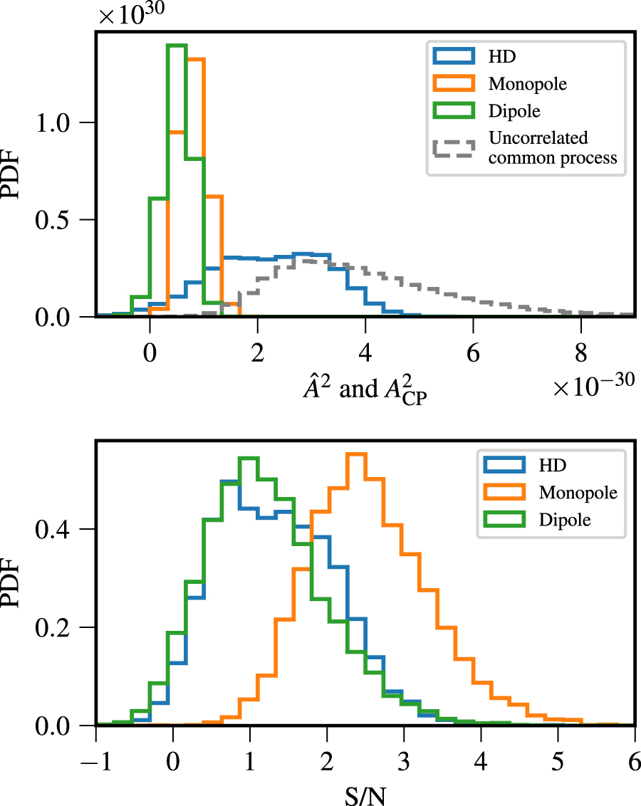