Rings and Gaps in Protoplanetary Disks: Planets or Snowlines?

In the last few years, Atacama Large Millimeter/submillimeter Array (ALMA) has revolutionized the field of study of protoplanetary disks, the birth cradles of planets. High-resolution imaging has revealed that the continuum emission of the millimeter-dust grains is not smooth, but consists of multiple dust rings. The most well-known example is the young HL Tau disk (ALMA Partnership et al. 2015), the first disk resolved at 25 mas resolution at millimeter wavelengths. Other disks showing multiple rings are, for example, TW Hya (Andrews et al. 2016), HD 163296 (Isella et al. 2016), HD 169142 (Fedele et al. 2017), AA Tau (Loomis et al. 2017), and AS 209 (Fedele et al. 2018). Even in lower-resolution data (∼02), evidence for outer dust rings is often found, for example, in HD 100546 (Walsh et al. 2014), RXJ 1615-3255 (van der Marel et al. 2015), and HD 97048 (van der Plas et al. 2017).

Whereas these rings and gaps are clearly common, the mechanism to explain the origin of the gaps remains unclear. Proposed scenarios include dust growth in condensation zones or snowlines (Zhang et al. 2015), zonal flows (Flock et al. 2015), self-induced dust pile-ups (Gonzalez et al. 2017), aggregate sintering (Okuzumi et al. 2016), large-scale instabilities (Lorén-Aguilar & Bate 2016) or secular gravitational instabilities (Takahashi & Inutsuka 2016) and, most popular, clearing by embedded planets (e.g., Lin & Papaloizou 1979; Kley & Nelson 2012; Baruteau et al. 2014), including the triggering of multiple gaps by a single planet (Bae et al. 2017; Dong et al. 2017a). However, the detections of planets embedded in disks are rare (e.g., Kraus & Ireland 2012; Quanz et al. 2013; Currie et al. 2015; Sallum et al. 2015) and often only upper limits can be set (Testi et al. 2015; Maire et al. 2017; Pohl et al. 2017). On the other hand, giant planets at wide orbits are rare (Bowler 2016) and the observed structures may be caused by currently undetectable, low-mass planets (Dong et al. 2015; Rosotti et al. 2016; Dipierro & Laibe 2017; Dong & Fung 2017). Furthermore, the commonality of ring structures at the very early and very late stages of protoplanetary disks (<1 to >10 Myr) casts doubts on the explanation of planets, as planets would need to be formed in ≪1 Myr timescales, well below current predictions of planet formation theory (Helled et al. 2014).

In order to understand the origin of the gaps, the structure of the gas needs to be known: whereas planets are expected to lower the gas density inside the gaps, other effects such as snowlines would not change the density itself. Gas cavities (linked to giant planets) have been revealed through CO observations in transition disks with large dust cavities (e.g., van der Marel et al. 2016; Dong et al. 2017b; Fedele et al. 2017), but the gas structure inside these narrow gaps has remained difficult to constrain. Gas gaps have been claimed through CO 2–1 isotopologue data in HD 163296 (Isella et al. 2016). In their modeling procedure, both the CO abundances and gas temperatures were parametrized. The depth of these gaps can be linked directly to planet masses of embedded planets (Fung et al. 2014; Rosotti et al. 2016; Dong & Fung 2017). Isella et al. (2016) deduced that ∼Saturn mass planets must be responsible for the gap structure, based on the depth of the gas gaps. However, kinematic signatures point toward more massive, Jupiter-like planets (Teague et al. 2018) inside the gaps, and direct imaging with Keck/NIRC2 has revealed a point source at 05 consistent with a Jupiter-like planet as well (Guidi et al. 2018).

Clearly, gaps in CO emission cannot be converted directly into gas surface density drops: the CO abundance is not constant with respect to H₂ throughout the disk due to, for example, photodissociation, freeze out, and chemical effects, and the gas temperature is decoupled from the dust temperature in the bulk of the disk depending on the local conditions, due to various heating-cooling effects (van Zadelhoff et al. 2001; Aikawa et al. 2002). The gas temperature can be up to two orders of magnitude higher in the disk atmosphere (Bruderer et al. 2012; Bruderer 2013). Recently, Facchini et al. (2018) showed that the gas temperature is in fact lower inside gas gaps created by giant planets due to the low dust-to-gas ratio and consequently, decreased gas-dust energy transfer, using the DALI code including dust evolution (Bruderer 2013; Facchini et al. 2017). This implies that care should be taken when drops in CO emission are observed. A physical–chemical model is thus crucial to interpret the complex structure CO emission properly.

In this Letter, we present the modeling outcome of two mechanisms for a dust ring disk, using the DALI code with a parametrized density structure. We show how the CO emission changes due to the presence of dust gaps on one hand, and due to changing in the grain-size distribution on the other hand. We discuss the implications for constraining the origin of dust rings from high-resolution CO observations.

The DALI code (Bruderer et al. 2012; Bruderer 2013) was developed for the prediction of molecular line fluxes of protoplanetary disks, for a given surface density structure of gas and dust and a given stellar spectrum providing the radiation field. DALI solves for the dust radiative transfer, the chemical abundance, the molecular excitation, and the thermal balance to obtain the gas temperature and CO abundances at each position in the disk. Further details on the parameters and assumptions in DALI are given in Bruderer (2013).

For our model, we mimic the structure of the HD 163296 disk as analyzed by Isella et al. (2016). The most recent parallax of HD 163296 is 9.85 ± 0.11 mas using Gaia data release 2 (DR2), corresponding to a distance of 101.5 ± 1.2 pc (Gaia Collaboration et al. 2018). As the old distance was 122 pc (van den Ancker et al. 1997), the gap radii and the stellar luminosity as derived by Isella et al. (2016) are scaled accordingly. We do not aim to provide a perfect fit to the observations, but use the structure to illustrate how the CO emission changes due to changes in the dust structure (left two panels of Figure 1). We use the same data images as presented in Isella et al. (2016) for our comparison. In order to enhance the visibility of the ring features, for each image we compute the ratio between the original and a smoothed version (smoothing FWHM is twice the beam size of the observations) and normalize the result. Both these enhanced image representation (EIR) and original images are provided to compare with the models. The central deficit in the ¹³CO and C¹⁸O images is not a real gap in the CO, but is caused by the continuum subtraction (see the discussion in Boehler et al. 2017).

Zoom In Zoom Out Reset image size

For the model, we assume a surface density profile Σ(r) as a radial power law with exponential cutoff following Lynden-Bell & Pringle (1974):

$$\begin{eqnarray}&&{\rm{\Sigma }}(r)={{\rm{\Sigma }}}_{c}{\left(\displaystyle \frac{r}{{r}_{c}}\right)}^{-\gamma }\exp \left(-{\left(\displaystyle \frac{r}{{r}_{c}}\right)}^{2-\gamma }\right)\end{eqnarray} \tag{ 1 }$$

with γ = 1. The dust surface density is computed by dividing the equation by the gas-to-dust ratio. Settling is parametrized following Bruderer (2013), with the scale height of the large grains distributed at a fraction of the total scale height. Furthermore, we assume the dust gap radial locations as derived in Isella et al. (2016) scaled to the new Gaia distance of 101.5 pc. The assumed parameters and properties of HD 163296 are summarized in Table 1 and the observational properties in Table 2. Stellar parameters are taken from Mendigutía et al. (2013).

The model is set up in two different ways: in Model A ("gap model") the dust surface density is decreased by a factor 0.010, 0.014, and 0.17 for gap r₁, r₂, and r₃, respectively, whereas the gas surface density is decreased by a factor 0.4, 0.29, and 0.56, respectively, following the dust and gas model of Isella et al. (2016). In Model B ("snowline model"), the dust surface density remains the same, but the fraction of large grains in the midplane f_ls is set to 0.01 inside of the three gaps, and otherwise f_ls = 0.99, to mimic increased dust growth in the rings and a deficit of large grains in the gaps. The two dust populations used in DALI are the small grain population (0.005–1.0 μm) and large grain population (0.005–1000 μm), and f_ls corresponds to the mass fraction of the large grains with respect to the total mass of dust grains. Note that in Model A f_ls was set constant at 0.85. This model mimics the dust size distribution as calculated from dust evolution models by Pinilla et al. (2017), where the large grain fraction is higher at certain radii as the result of snowlines and the resulting change in fragmentation velocity. The radii are chosen based on the observed ring radii rather than the actual temperature profile at this point.

Snowlines are expected to induce pressure bumps in viscosity gradients due to the change in the gas ionization fraction as a result of the change in chemistry (e.g., Flock et al. 2015), which results in dust traps as well. As the calculation of the efficiency of this effect is beyond the capabilities of DALI, no additional change in gas or dust surface density is introduced in Model B. The choice of f_ls = 0.01 is justified by testing a range of models with different values for f_ls: a value of 0.01 or lower is required to reproduce the dust continuum contrast seen in the rings of the observations. Values of 10⁻²–10⁻⁴ have been tested, and the difference in CO emission is negligible. In addition, we have run Model 0 without any radial changes in the surface density or grain size distribution, and a variation of Model A with much deeper gaps (Model C). Figure 3 shows the structure in each model.

DALI was run using a grid with 190 cells in radial and 60 cells in vertical direction, using time-dependent chemistry up to 1 Myr. The additional DALI modules with isotope-selective photodissociation (Miotello et al. 2014) were not included in all models, but this is not expected to change the main results.

Figure 1 shows the comparison of the dust image in EIR with both models. Both models are capable of reproducing the dust ring morphology seen in the data, with normalized dips as low as 40% of the maximum.

In Figure 2 the resulting CO emission for both models is shown for all three CO isotopologues. The inner part (<025) can be ignored as this is dominated by the continuum oversubtraction. The modeling does not try to account for this effect with an exact fit to the continuum, and is focused on the rings, not the center. The images are shown in EIR. In the azimuthally averaged cuts it immediately becomes apparent that the snow model results in marginal radial changes, only due to the continuum oversubtraction, while the gap model shows strong incremented rings in the CO. Remarkably, even though the gas surface density has been decreased inside the dust gaps, the CO emission (in particular the C¹⁸O) is brighter. In order to understand this phenomenon, a more detailed look into the physics and chemistry in the disk is required.

Zoom In Zoom Out Reset image size

Figure 3 shows the structure of each model as calculated by DALI. Both models are compared with a model of similar disk mass where no gaps in dust or gas are introduced (Model 0).

Zoom In Zoom Out Reset image size

Comparing the models in Figure 3 reveals several remarkable differences in the temperature structure when gaps are introduced. Both T_gas and T_dust increase inside the gaps due to an increase in the ultraviolet (UV) field (G₀). The ratio T_gas/T_dust slightly decreases in the surface layers, but not in the bulk region below the surface. We note that the temperature inversion in the thin upper surface layer (above the hot layer) in the T_gas is not relevant for the molecular gas temperature, as molecules such as CO and H₂ are photodissociated here.

The increase in T_gas inside the gaps results in a decrease of frozen-out CO molecules: in Model A, CO is abundant all the way down to the midplane in the gaps, whereas Model 0 shows that CO starts to be frozen out from 60 au onward if no gaps are introduced. This leads to an increase in CO abundance inside the gaps, which produces the bright CO rings seen in Figure 2. The CO emission is increased more for the less abundant C¹⁸O than for ¹²CO, consistent with an abundance increase. This can only be explained by a marginal change in gas temperature in combination with a large change in abundance, as even the C¹⁸O emission is marginally optically thick. Isotope-selective photodissociation (Miotello et al. 2014) does not significantly change the outcome due to the high CO abundances.

Results of hydrodynamic simulations of planet–disk interactions show an additional increase of the gas temperature up to 50% in the gap as the result of the planet presence, as hydrostatic equilibrium needs to be maintained at a gap edge (Isella & Turner 2018, their Figure 6), which further strengthens this case. As a combination of physical–chemical modeling to the level of DALI together with hydrodynamical simulations such as in Isella & Turner (2018) is computationally unfeasible, it is not possible to calculate the combined effect quantitatively.

Model B, on the other hand, does not show any changes in temperature, UV, or CO abundance structure despite the radial changes in the dust grain size distribution, which is consistent with what is seen in the CO images in Figure 2. The snow model can thus reproduce dust rings without changing the CO emission itself.

Both the gap model and snow model can reproduce the morphology of the continuum image, reducing the emission inside the gaps similar to the data. However, the CO emission can distinguish between the two models: a snow model does not show any significant radial changes in the CO emission, whereas a gap model can result in increased CO emission inside of the gap due to increased gas temperature, depending on the gap depth. The image data does not show an increase of emission inside the gaps, so the estimated density gap depths by Isella et al. (2016) are likely underestimated.

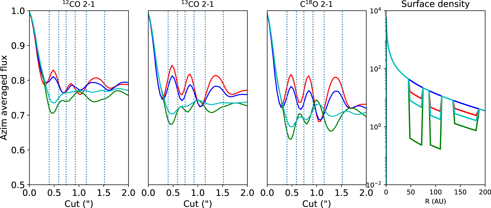
In order to investigate how deep the gas gaps need to be in order to decrease the CO emission inside the gaps, a number of models with different δ_gas are run and presented in Figure 4. The values of δ_gas range between 1 and 10⁻². The deeper gap appears to be more consistent with the data. The gap depth in gas generally scales with the planet mass (Fung et al. 2014; Kanagawa et al. 2015): a deeper gap results in a larger planet masses. Isella et al. (2016) estimated Saturn-like planet masses of 0.1, 0.3 and 0.3 M_Jup, respectively, based on their gap depths, but our models suggest that the gaps, if caused by planets, must contain planets that are at least a Jupiter mass. This is also consistent with the findings of the kinematics (Teague et al. 2018). Furthermore, the larger planet masses are more consistent with the observed gap widths, which are ∼25 au. Planets of ∼0.1 M_Jup are expected to open gaps of only a few au wide (e.g., Dong & Fung 2017), depending on the α viscosity. Isella et al. (2016) proposed multiple planets to be responsible for the wider gaps. However, if the dust is trapped in pressure maxima, the width of the dust gaps may be overestimating the actual gaps opened by the planet.

Zoom In Zoom Out Reset image size

An observational distinction between the two models remains challenging: the density drops change the radial CO emission depending on the depth, but if the emission shows only no significant radial variations, then both a shallow gap and snow model remain possible. However, it is also still possible that a single planet is responsible for multiple gaps, if the viscosity of the disk is very low (Dong et al. 2017a), but there is no observational difference in the gas surface density in this case.

Another interesting question is what happens to the gas temperature in very deep gaps. Facchini et al. (2018) have shown that a gap created by a Jupiter-mass planet creates a gap almost completed by dust, increasing the gas-to-dust ratio inside the gap, which results in T_gas < T_dust in the entire gap due to the thermal decoupling between gas and dust. In the rightmost panel of Figure 3 we explore this scenario, with a drop in dust density of 10⁻⁵ and gas density of 10⁻³ inside of the gaps. The temperature inversion inside the gaps is reproduced, but as there is so little dust in the gaps, there is no increase in frozen-out CO molecules in this case. The low gas surface density (and resulting low CO abundance) results in deep CO gaps.

In summary, CO emission in dust gaps due to planets are complicated to interpret and one has to be careful when examining either the increase or decrease of emission inside of the gap. When no radial change is visible in the CO emission, this can be either a specific gas surface density drop or an indicator of a snowline, as shown in Figure 2. As the interpretation of the data of HD 1632926 is inconclusive about the presence of gaps in CO, the snowline scenario is still a possibility. This would also be more consistent with the observed presence of gaps and rings across the wide range of disk ages (0.4–10 Myr).

In order to explore the possibility of snowlines in HD 163296, we check the gas temperatures close to the midplane of Model B and compare them with condensation temperatures of molecules commonly found in disks, similar to the procedure in HL Tau by Zhang et al. (2015).

Figure 5 shows the midplane temperature as a function of radius, with the gaps indicated. The parametrized midplane temperature used by Isella et al. (2016) is also plotted, which is almost identical to the temperature calculated by our radiative transfer code. On top of this plot, we show the regions where CO, CO₂, and CH₄ are expected to be frozen out, based on the condensation temperatures derived in Table 2 in Zhang et al. (2015): 23–28 K for CO, 26–32 K for CH₄, and 60–72 K for CO₂, respectively. Furthermore, we overlay the snowline as derived from N₂H⁺ and DCO⁺ observations (Qi et al. 2011) in HD 163296, located at 75 ± 6 au.

It is clear that the CH₄ freeze-out region overlaps with the first gap, and the CO freeze-out region with the second gap; this is even further motivated by the location of the snowline as derived from the N₂H⁺ data. The CO₂ freeze-out region does not overlap with a dust gap, but at this radius the dust is very optically thick so radial variations would not be visible, or perhaps remain unresolved. No molecule is known to freeze out in the temperature range of the third gap (18–20 K), but it is possible that the estimates for the condensation temperature N₂ are slightly underestimated in Zhang et al. (2015) at 12–16 K and the region is actually coinciding with that condensation region. Gaps caused by freeze-out zones may appear to be controversial, but this implies that the increased stickiness at these radii results in growth of dust particles well beyond millimeter sizes, hence creating dips in the millimeter continuum emission. In that case, rings are simply the region where millimeter grains still remain. This is the opposite of our Model B and the results of Pinilla et al. (2017), where the snowline is suggested to coincide with the ring location rather than the gap location. Growth up to decimal sizes to explain gaps in dust images was originally proposed by Zhang et al. (2015). The uncertainties in parameter choices such as viscosity, gas surface density, and timescales imply that growth to decimal sizes cannot be excluded.

Zoom In Zoom Out Reset image size

For HD 163296, the origin of the dust gaps thus remains unclear. Deeper CO observations at high spatial resolution are required to see whether or not gaps can be ruled out. This study shows the complicated nature of CO emission inside gaps, and the need for full physical–chemical modeling to interpret the underlying gas density.

The authors would like to thank Andrea Isella and Greta Guidi for providing the reduced fits cubes of HD 163296. This research was supported by the Munich Institute for Astro- and Particle Physics (MIAPP) of the DFG cluster of excellence "Origin and Structure of the Universe. This Letter makes use of the following ALMA data: ADS/ JAO.ALMA#2013.1.00601.S. ALMA is a partnership of ESO (representing its member states), NSF (USA) and NINS (Japan), together with NRC (Canada) and NSC and ASIAA (Taiwan), in cooperation with the Republic of Chile. The Joint ALMA Observatory is operated by ESO, AUI/NRAO and NAOJ.

The appendix provides the modeling parameters used for calculating the models (Table 1) and the observational properties of the data (Table 2).

Table 1.  Model Parameters

Parameter	Value	Description
Stellar	L*	20.8 L⊙	Stellar luminosity
	Teff	9250 K	Stellar temperature
	${\dot{M}}_{\mathrm{acc}}$	10−6.3 M⊙ yr−1	Accretion rate
	d	122 pc	Distance
Disk	Mgas	3.9 × 10−1 M⊙	Disk gas mass
	Mdust	3.9 × 10−3 M⊙	Disk dust mass
	rc	150 au	Critical radius
	Σc	25 g cm−2	Surface density at rc
	hc	0.05	Scale height
	ψ	0.1	Flaring angle
	rout	450 au	Outer radius
Gaps	r1	40–60 au	Dust gap 1
	r2	74–92 au	Dust gap 2
	r3	114–151 au	Dust gap 3

Download table as:  ASCIITypeset image

Table 2.  Observational Properties

Component	Ftot,data	Beam Size	${F}_{\mathrm{tot},\mathrm{snowmodel}}$	${F}_{\mathrm{tot},\mathrm{gapmodel}}$
	(Jy km s−1)	('')	(Jy km s−1)	(Jy km s−1)
Continuum (230 GHz)	0.732	0.25 × 0.25	0.95	1.27
12CO 2–1	41.05	0.22 × 0.16	25.50	25.65
13CO 2–1	15.53	0.23 × 0.17	10.47	10.78
C18O 2–1	5.46	0.24 × 0.17	4.465	4.471

Download table as:  ASCIITypeset image