


Abstract
We present our observations of electromagnetic transients associated with GW170817/GRB 170817A using optical telescopes of Chilescope observatory and Big Scanning Antenna (BSA) of Pushchino Radio Astronomy Observatory at 110 MHz. The Chilescope observatory detected an optical transient of ∼19m on the third day in the outskirts of the galaxy NGC 4993; we continued observations following its rapid decrease. We put an upper limit of 1.5 × 10⁴ Jy on any radio source with a duration of 10–60 s, which may be associated with GW170817/GRB 170817A. The prompt gamma-ray emission consists of two distinctive components—a hard short pulse delayed by ∼2 s with respect to the LIGO signal and softer thermal pulse with T ∼ 10 keV lasting for another ∼2 s. The appearance of a thermal component at the end of the burst is unusual for short GRBs. Both the hard and the soft components do not satisfy the Amati relation, making GRB 170817A distinctively different from other short GRBs. Based on gamma-ray and optical observations, we develop a model for the prompt high-energy emission associated with GRB 170817A. The merger of two neutron stars creates an accretion torus of ∼10−2 M⊙, which supplies the black hole with magnetic flux and confines the Blandford–Znajek-powered jet. We associate the hard prompt spike with the quasispherical breakout of the jet from the disk wind. As the jet plows through the wind with subrelativistic velocity, it creates a radiation-dominated shock that heats the wind material to tens of kiloelectron volts, producing the soft thermal component.
Export citation and abstract BibTeX RIS
1. Introduction
On 2017 August 17 at 12:41:04 UTC, the LIGO-Hanford detector triggered the gravitational-wave (GW) transient GW170817 (LIGO Scientific Collaboration & Virgo Collaboration 2017). The GW signal was also found in the data of other LIGO and Virgo detectors and was consistent with the coalescence of a binary neutron star system coalescence. Two seconds later (UTC 2017 August 17 12:41:06) GRB 170817A was registered by GBM/Fermi (Goldstein et al. 2017a, 2017b; Connaughton et al. 2017) and SPI-ACS/INTEGRAL (Savchenko et al. 2017a, 2017b) experiments. The GBM/Fermi localization area of GRB 170817A includes the much smaller localization region of GW170817. A search for the optical counterpart started immediately and was carried out by a large number of ground-based facilities (LIGO Scientific Collaboration et al. 2017).
2. Optical Observations
The optical transient corresponding to GW170817 and GRB 170817A was discovered independently by several observatories. The first team to discover and report the detection of the optical counterpart was The One-Meter, Two-Hemisphere (1M2H) group. They detected a bright uncataloged source within the halo of the galaxy NGC 4993 in their i-band image obtained on 2017 August 17 23:33 UTC with the 1 m Swope telescope at Las Campanas Observatory in Chile. This source was labeled as Swope Supernova Survey 2017a (SSS17a; Coulter et al. 2017, notice time 2017 August 18 01:05 UTC). SSS17a (now with the IAU designation AT2017gfo) had coordinates R.A.(J2000.0) = 13h09m48 085 ± 0.018, decl.(J2000.0) = −23°22'53
 343 ± 0.218 and was located at a projected distance of 106 from the center of NGC 4993, an early-type galaxy at a distance of ≃40 Mpc. Hereafter, we refer to the optical counterpart as OT.
The Distance Less Than 40 Mpc survey (DLT40; L. Tartaglia et al. 2017, in preparation) obtained their first image of NGC 4993 region on 2017 August 17 23:50 UTC and independently detected the transient, automatically labeled DLT17ck (Yang et al. 2017, notice time August 18, 01:41 UTC).
MASTER-OAFA robotic telescope (Lipunov et al. 2010) observed the region including NGC 4993 on August 17 23:59 UTC, and the automated software independently detected the transient labeled MASTER OT J130948.10-232253.3 (Lipunov et al. 2017, notice time August 18 05:38 UTC).
Visible and Infrared Survey Telescope for Astronomy (VISTA) also observed the transient SSS17a/DLT17ck/MASTER OT J130948.10-232253.3 in the infrared band on August 18, 00:10 UT (Tanvir & Levan 2017, notice time August 18, 05:04 UTC).
Las Cumbres Observatory (Brown et al. 2013) surveys started observations of the Fermi localization region immediately after the corresponding GCN circular distribution. Approximately 5 hr later, when the LIGO-Virgo localization map was issued, the observations were switched to the priority list of galaxies (Dalya et al. 2016). On August 18 00:15 UTC, a new transient near NGC 4993 was detected at the position corresponding to the OT (Arcavi et al. 2017, notice time August 18, 04:07 UTC).
The team of DECam on the 4 m telescope of Cerro Tololo Inter-American Observatory independently detected in optics the new source north and east of NGC 4993 in the frame taken on August 18, 00:42 UTC (Allam et al. 2017, notice time August 18, 01:15 UTC).
We started observations of the error box of GW170817 (LIGO/Virgo trigger G298048) on August 17 23:17:16 UTC (Pozanenko et al. 2017a, notice time August 18, 14:24 UTC) with the facilities of the Chilescope observatory (see Appendices A.1 and A.2). Simultaneously, we started mosaic observations of GBM/Fermi localization area of GRB 170817A (von Kienlin et al. 2017), taking a series of spatially tiled images with another instrument of the same observatory (see Appendix A.3). The observations ended ∼5 minutes before the GCN circular about the discovery of the transient was distributed by Swope (Coulter et al. 2017). The location of NGC 4993 was out of the covered fields of our first observational set.
We started to observe the optical counterpart of the GW170817 (LIGO Scientific Collaboration & Virgo Collaboration 2017) labeled SSS17a (Coulter et al. 2017) on 2017 August 19 at 23:30:33 with RC-1000 telescope of Chilescope observatory (Pozanenko et al. 2017c) and continued observations on 2017 August 20, 21, and 24. Details of our optical observations and data reduction are presented in Appendices A.4 and A.5. The final light curve in the R-filter incorporating our photometry result are presented in Appendix A.6. We also compared the light curves of the afterglow of GRB 130603B with the light curve of the optical counterpart of GRB 170817A and found that the afterglow luminosity of GRB 170817A is more than 130 times fainter than that of GRB 130603B in the J-filter (see A.6). We used data of the Big Scanning Antenna (BSA) radio telescope survey at 110 MHz to estimate the possible radio prompt emission. Details of our radio observations are presented in Appendix B.
3. GRB 170817A Prompt Gamma-Ray Data Analysis
3.1. SPI-ACS/INTEGRAL
The description of GRB 170817A INTEGRAL observations and detailed analysis of the burst based on INTEGRAL data are presented in Savchenko et al. (2017a). We performed a basic analysis of the SPI AntiCoincidence Shield (SPI-ACS) data with a slightly different method to classify the burst and to estimate its energetics, and then compare our results with those of GBM/Fermi in order to calibrate SPI-ACS consequently. We found the burst to be from a short (or Type I) population with no precursor and extended emission components. Derived values of fluxes in energetic units are consistent with both our GBM/Fermi and Savchenko et al.'s (2017a) results. The time delay between the burst onset and GW trigger was found to be ≃2 s. The background-subtracted light curve of the burst in SPI-ACS data with a time resolution of 0.2 s is shown in Figure 1(e). The details of the analysis are presented in Appendix C.

Figure 1. Background-subtracted dynamic count spectrum (a) and light curves of GRB 170817A in data of GBM/Fermi (Nai: 1, 2, 5) in (8, 50) keV (b), (50, 100) keV (c), (100, 300) keV (d), and in data of SPI-ACS/INTEGRAL (e). Time in seconds since GW trigger (UTC 2017 August 17 12:41:04) is on the X-axis, counts over 0.2 s time bins are on the y-axis for light curves. Flux uncertainties are presented at the 1σ significance level. A warmer color on the dynamic count spectrum (a) corresponds to a higher flux. The two-component (pulse) structure of GRB 170817A is seen. For the first pulse, the red line represents logarithmic spectral lag behavior on energy, lag ∼ 0.24 × log(E). The logarithmic approximation is typical for single pulses of GRBs (Minaev et al. 2014).
Download figure:
Standard image High-resolution image3.2. GBM/Fermi
We used the publicly accessible FTP archive9 as the source of the GBM/Fermi data.
GRB 170817A was detected in GBM/Fermi (Nai: 1, 2, 5) at the 8.7σ significance level in the (8, 300) keV energy range. The background-subtracted dynamic count spectrum in the (8, 400) keV range and light curves of the burst with time resolution of 0.2 s are presented in three energy channels in Figures 1(a)–(d). The burst onset in GBM/Fermi data is delayed by ≃2 s compared to the GW trigger. The third-order polynomial model was used to fit background in time intervals (−40, −5) and (20, 70) s for all presented GBM/Fermi light curves.
As seen in Figure 1, light curve of the burst consists of two different components (pulses): the first one is short hard and the second one is visible only in soft energy range (8, 50) keV. The two-component structure of the burst is also confirmed by T90 duration parameter values: in the (8, 70) keV energy range  , which is six times longer than the duration in the (70, 300) keV energy range,
  . (That behavior cannot be explained by the well-known dependence of GRB duration on energy range, T90 ∝ E−0.4; see, e.g., Fenimore et al. 1995; Minaev et al. 2010b).
To construct and fit the energy spectra, we used the RMfit v4.3.2 software package10 developed to analyze the GBM data of the Fermi observatory. The method of spectral analysis is similar to that proposed by Gruber et al. (2014), who also used the RMfit software package. To fit the energy spectra and to choose an optimal spectral model, we used modified Cash statistics (C-Stat; see Cash 1979).
Results of spectral analysis performed for GRB 170817A using data of GBM/Fermi (Nai: 1, 2, 5, BGO: 0) are summarized in Table 1. We analyzed three time intervals covering the whole burst—(−0.3, 2.0) s since GBM trigger, the first hard pulse (−0.3, 0.3) s, and the second soft pulse (0.8, 2.0) s—with three spectral models—power law (PL), power law with exponential cutoff (CPL), and thermal model (BB). To choose the optimal spectral model, we used the ΔC-Stat > ΔC-Statcrit criterion, where ΔC-Stat is the difference between C-Stat values obtained for various models (the last column in Table 1) and ΔC-Statcrit ≃ 8.5 was obtained via simulations in Gruber et al. (2014) for PL versus CPL model comparison.
Table 1. Results of Spectral Analysis of GRB 170817A Based on GBM/Fermi Data
| Time Intervala | Modelb | α | Epeakc | Fluenced | Hardness Ratioe | C-Stat/dof |
|---|---|---|---|---|---|---|
| (s) | (keV) | (10−7 erg cm−2) | ||||
| (−0.3, 0.3) | PL | −1.50 ± 0.08 | ... | 2.8 ± 0.4 | 0.72 ± 0.13 | 425/367 |
| first | BB | ... | 31.6 ± 3.2 | 1.4 ± 0.2 | 2.8 ± 0.6 | 437/367 |
| pulse | CPLf | −0.9 ± 0.4 |

|
2.2 ± 0.5 | 1.0 ± 0.2 | 416/366 |
| (0.8, 2.0) | PL | −2.0 ± 0.3 | ... | 1.0 ± 0.4 | 0.37 ± 0.15 | 439/367 |
| second | BBf | ... | 11.2 ± 1.5 | 0.68 ± 0.11 | 0.24 ± 0.09 | 422/367 |
| pulse | CPL |

|

|
0.67 ± 0.12 | 0.23 ± 0.10 | 422/366 |
| (−0.3, 2.0) | PL | −1.8 ± 0.1 | ... | 3.7 ± 0.7 | 0.49 ± 0.09 | 450/367 |
| whole | BB | ... | 13.3 ± 1.3 | 1.7 ± 0.2 | 0.39 ± 0.08 | 447/367 |
| burst | CPLf |

|

|
2.1 ± 0.3 | 0.46 ± 0.09 | 440/366 |
Notes.
aTime interval relative to GBM trigger (UTC 2017 August 17 12:41:06.475). bPL is for power law, CPL is for power law with an exponential cutoff, and BB is for a thermal model. cFor the BB spectral model, the Epeak column gives the parameter kT. dFluence in the (10, 1000) keV energy range. ehardness ratio calculated as a ratio of photon fluxes in (50, 300) keV and (15, 50) keV energy bands. foptimal spectral model.Download table as: ASCIITypeset image
The energetic spectrum of the whole burst (time interval (−0.3, 2.0) s) is best fitted by the CPL model with  and
and  (the improvement over PL model is ΔC-Stat = 10). The fluence in the (10, 1000) keV range is F = (2.1 ± 0.3) × 10−7 erg cm−2. Using the CPL spectral model, we calculated the hardness ratio of photon fluxes between (50, 300) keV and (15, 50) keV energy bands, HR = 0.46 ± 0.09, which, along with duration
  , characterizes the burst to be a typical short but soft one (e.g., see Figure 6 in von Kienlin et al. 2014). The probability that GRB 170817A is from the short population was estimated using duration and hardness values in Goldstein et al. (2017a) and found to be P ≃ 73%.
The optimal spectral model for the first pulse (time interval (−0.3, 0.3) s) of the GRB 170817A is the CPL model (Table 1) with α = −0.9 ± 0.4 and  (the improvement over the PL model is ΔC-Stat = 9). Using the CPL spectral model, we calculated a hardness ratio between (50, 300) keV and (15, 50) keV energy bands, HR = 1.0 ± 0.2, which describes the first pulse as a hard one (see Figure 6 in von Kienlin et al. 2014).
The optimal spectral model for the second pulse (time interval (0.8, 3.0) s) of the GRB 170817A is a thermal model with kT = 11.2 ± 1.5 keV and the fluence is in the (10, 1000) keV energy range of F = (6.8 ± 1.1) × 10−8 erg cm−2 (Table 1). The CPL model gives the same goodness of fit, but with a positive value of  , bringing this model maximally close to Wien's law NE ∼ E2 exp(−E/kT)—the spectral shape that the radiation originating in an optically thick hot medium whose opacity is dominated by Compton scattering off electrons acquires (Kompaneets 1957), which also confirms the thermal nature of the second pulse. The
  parameter was found to be
  within the CPL model. The improvement of C-Stat for CPL and BB models comparing to the PL one is ΔC-Stat = 17, which is two times larger than ΔC-Statcrit ≃ 8.5 found in Gruber et al. (2014) and used as model selection criterion. Within the CPL model, the hardness ratio between (50, 300) keV and (15, 50) keV energy bands, HR = 0.23 ± 0.10, which describes the second pulse to be a very soft one (see Figure 6 in von Kienlin et al. 2014).
Optimal spectral models are presented in Figures 2 and 3, while confidence regions of the parameters of CPL models for both pulses are presented in Figure 4. As can be seen from Figure 4, the spectrum describing these two pulses is not evolving, but rather is a manifestation of the different nature of the emission. The results of our spectral analysis are comparable with ones presented in Goldstein et al. (2017a).

Figure 2. Photon spectrum (upper panel) and residuals (lower panel) of the CPL spectrum model for the first pulse.
Download figure:
Standard image High-resolution image
Figure 3. Photon spectrum (upper panel) and residuals (lower panel) of the black body spectrum model for the second pulse. The dashed line represents the CPL fit of the photon spectrum.
Download figure:
Standard image High-resolution image
Figure 4. Confidence regions at the 1, 2, 3σ levels of the CPL spectrum parameters (power-law index, α and Epeak) for the first and second pulses.
Download figure:
Standard image High-resolution imageWe did not find any precursor or extended emission components in GBM/Fermi data at timescales from 0.1 up to 20 s in the time interval (−10, 30) s since GBM triggers in the energy range of (8, 300) keV. To estimate upper limits on their intensity in energetic units, we derived a conversion factor in the (8, 300) keV range using count fluence of the burst and energetic fluence within CPL spectral model (Table 1). We found that 1 count in GBM/Fermi corresponds to ∼3.2 × 10⁻¹⁰ erg cm−2 in an energy range of (8, 300) keV. At a timescale of 0.1 s, the upper limit on precursor activity is Sprec ≃ 1.6 × 10⁻⁸ erg cm−2 at the 3σ significance level. At a timescale of 20 s, the upper limit on extended emission activity is SEE ≃ 2.3 × 10⁻⁷ erg cm−2 at a 3σ significance level. The upper limits are two times deeper than ones obtained with SPI-ACS (see Appendix C).
A spectral lag analysis based on the CCF method (see, e.g., Minaev et al. 2014) was performed for GRB 170817A using the light curves detected by GBM/Fermi (Nai: 1, 2, 5) in the energy bands (8, 50) keV, (50, 100) keV, and (100, 300) keV with a time resolution of 0.04 s. The spectral lag between (8, 50) keV and (50, 100) keV bands is negligible, lag = 0.01 ± 0.08 s, but between (8, 50) keV and (100, 300) keV lag is significant, lag = 0.27 ± 0.05 s. It might represent the hard-to-soft spectral evolution of the first pulse (see Figure 1(a)).
3.3. Amati Relation
One of the interesting phenomenological relations for GRBs is the Amati diagram, i.e., the dependence of the equivalent isotropic energy Eiso emitted in gamma-rays between (1, 10,000) keV on parameter  in the source frame (Amati 2010), which can also be used for the classification of GRBs (e.g., Qin & Chen 2013).
Using the experimental data given in Svinkin et al. (2016), Qin & Chen (2013), and Minaev & Pozanenko (2017), we constructed the Amati diagram for 20 short bursts and fitted the relation with a power-law-like logarithmic model:  . Details on the investigation of the Amati relation for short GRBs can be found elsewhere (P. Minaev 2018, in preparation).
Using optimal spectral models derived in the previous subsection for GRB 170817A (Table 1) and assuming a redshift of z = 0.00968 and a luminosity distance of DL = 42.0 Mpc for the source (Jones et al. 2009), we estimated Eiso and Liso parameters in the (1, 10,000) keV range (Table 2). All burst components (first, second pulses, and the whole burst) lie far above the 2σ correlation region (Figure 5).

Figure 5. Amati diagram; the dependence of the equivalent isotropic energy Eiso emitted in the (1, 10,000) keV range on Epeak(1 + z) in the source frame (Amati 2010), for short bursts. A power-law fit (thick solid line) with dashed lines bounding the 2σ region are shown. Dotted lines starting from the point for the whole GRB 170817A indicate the dependence  and
and  . Uncertainties for Eiso and Epeak(1 + z) are presented at the 1σ significance level.
Download figure:
Standard image High-resolution imageTable 2. GRB 170817A Energetics
| Time Intervala | Spectral | Fluxc | Fluenced |

|
Liso |
|---|---|---|---|---|---|
| (s) | modelb | 10−7 erg/(cm2 s) | 10−7 erg cm−2 | 1046 erg | 1046 erg s−1 |
| (−0.3, 0.3) | CPL | 3.8 ± 0.9 | 2.3 ± 0.9 | 4.9 ± 1.2 | 8.1 ± 1.9 |
| (0.8, 2.0) | BB | 0.59 ± 0.10 | 0.71 ± 0.12 | 1.5 ± 0.3 | 1.3 ± 0.2 |
| (0.8, 2.0) | CPL | 0.56 ± 0.10 | 0.67 ± 0.13 | 1.4 ± 0.3 | 1.2 ± 0.2 |
| (−0.3, 2.0) | CPL | 0.96 ± 0.14 | 2.2 ± 0.32 | 4.7 ± 0.7 | 2.1 ± 0.3 |
Notes.
aRelative to the GBM trigger (UTC 2017 August 17 12:41:06.475). bCPL is for power law with an exponential cutoff, BB for a thermal model. cEnergy flux in the (1, 10,000) keV energy range. dEnergy fluence in the (1, 10,000) keV energy range.Download table as: ASCIITypeset image
If we assume that the burst GRB 170817A should obey the Amati relation, we can draw a trajectory of the burst parameters as  if it is a cone relativistic jet emission, and
  if it is a spherical relativistic emission (see, e.g., Eichler & Levinson 2004; Levinson & Eichler 2005). One can see that neither of the trajectories cross the Amati relation at a reasonable Eiso, especially for the first pulse. This strongly supports an alternative explanation for the nature of the first pulse as well as the whole burst in comparison with the usual short GRBs presented in the Amati relation (Figure 5).
4. The Scenario
The key points of the model are illustrated in Figures 6–7.

Figure 6. Sketch of our scenario. After merging of NSs, a BH is formed, which is surrounded by a compact accretion disk with intense wind. After sufficient magnetic flux is accumulated on the BH an electromagnetic jet is launched, confined initially by the disk wind. After propagating with mildly relativistic velocities, the jet breaks out from the wind zone in a semi-isotropic fashion, reaching highly relativistic Lorentz factors. This is the prompt GRB.
Download figure:
Standard image High-resolution image
Figure 7. Post-breakout structure of the flow. The wind from the disk keeps collimating the jet for a few seconds. The jet propagates ballistically with Lorentz factors ≥20 and is unobservable due to deboosting. The shocked wind material produces thermal extended gamma-ray component with T ∼ 10 keV.
Download figure:
Standard image High-resolution imageThe detection of the EM signal contemporaneous with gravitational waves is consistent with the binary NS scenario for short GRBs (Blinnikov et al. 1984; Paczynski 1986; Eichler et al. 1989). Qualitatively, the evolution of merging neutron stars follows a well-defined path (e.g., Radice et al. 2016; Ruiz et al. 2016; Baiotti & Rezzolla 2017, and many others), though many details, like the effects of different equations of states, various mass ratios, initial spins, and magnetic field evolution, remain to be settled. An active stage of a merger lasts ∼10–100 milliseconds after which the neutron stars collapse into BH.11 The BH is fairly fast rotating with the Kerr parameter a ∼ 0.7 (Radice et al. 2016; Ruiz et al. 2016). The mass of the resulting BH is somewhat smaller than the sum of masses due to emission of neutrinos, gravitational waves, ejection of the tidal disruption tail, and wind from the accretion disk, so we can estimate it as MBH ≈ 2.5 M⊙. The amount of the ejected material is especially uncertain, but is of utmost importance for the production of the EM signal. It is expected that, first, tidal tails eject 0.01–0.03 M⊙ with outflow speed vex ≈ 0.1–0.3 c. This material is likely a site of r-process nucleosynthesis and can be seen as a kilonova—an optical emission of peak luminosity ∼1041 erg s −1 lasting for a few weeks (see Roberts et al. 2011; Barnes & Kasen 2013; Bauswein et al. 2013; Kasen et al. 2013; Grossman et al. 2014; Wanajo et al. 2014; Barnes et al. 2016; Wu et al. 2017).
Second, during the merger, an accretion torus of ∼0.01 M⊙ forms around the BH with viscous time 0.1 s (Radice et al. 2016; Ruiz et al. 2016; Baiotti & Rezzolla 2017). Highly different masses of merging NSs are good for the formation of a massive disk, which can enhance jet power and aid its confinement. This accretion disk plays the most important part in our model. For a few seconds, the disk undergoes viscous spreading, produces powerful neutrino-driven winds, and exercises accretion onto the BH via the inner edge (presumably close to the innermost stable orbit), see Section 6.1. Interestingly, in the case of BH+NS merging, the neutrino heating mechanism (Eichler et al. 1989; Birkl et al. 2007; Zalamea & Beloborodov 2011) can be the main source of the jet's energy (see Barkov & Pozanenko 2011). In the case of NS+NS merging, the mass of the accretion torus is relatively small (<10−2 M⊙), so the neutrino heating mechanism cannot be efficient on timescales of a few seconds.
At the same time, magnetic fields are amplified within the disk to ∼1015 G (Rezzolla et al. 2011) due to the development of MRI and the presence of the velocity shear. As the matter is accreted onto the BH, the BH accumulates magnetic flux. Accumulation of the magnetic flux leads to a delay for the jet to switch-on. At the same time, baryons slide off into the BH along magnetic field lines, leaving polar regions with low density. This creates conditions favorable for the operation of the Blandford–Znajek (BZ) mechanism (Blandford & Znajek 1977; Komissarov & Barkov 2009).
The BZ mechanism—production of EM outflows from the magnetic field supplied by the disk—also requires the presence of the external medium to produce jets (collimated outflows). It is the heavy baryonic wind from the disk that provides the required collimating surrounding. Importantly, the disk wind has only limited spatial extent—propagating with a velocity of  for about a few seconds it reaches out only to a few ×109 cm. Outside of the wind, the surrounding is very clean.
The BZ jet propagates through a dense wind with mildly relativistic velocity (Section 6.3). At the same time, the jet is mildly dissipative (Section 4.1; and thus highly optically thick). In a few seconds, the head of the EM jet reaches the edge of the wind. During the breakout, the head part of the jet expands with highly relativistic velocities in the direction of jet propagation and moderately relativistic velocities to the sides. Sudden expansion leads to pair annihilation and the production of gamma-ray emission in a manner similar to conventional models of GRBs (Section 4.1). This is the prompt GRB.
After the jet breaks out from the wind, a rarefaction wave propagating toward the BH leads to the acceleration of the jet, which loses internal causal contact and propagates nearly ballistically (Figure 7). Since the jet emission is highly debeamed, the jet becomes unobservable. The wind emission shocked by the breaking-out jet produces the soft tail (Figure 7).
A similar model for the formation of the first hard gamma-ray pulse was independently suggested in the paper by Gottlieb et al. (2017). This paper focuses on the effects of the jet breakout, both hydrodynamic and radiation processes.
4.1. Jet Breakout—Prompt Hard GRB
The BZ mechanism of jet launching requires clean plasma—there should be little mass loading and magnetic dissipation close to the source. This is indeed expected if the flow originates on field lines that penetrate the BH. It is expected that a jet launched by the BH is highly magnetized, σ ≫ 1. Importantly, the confined jet with σ ≫ 1 that propagates with non-relativistic velocity must necessarily be dissipative (Lyutikov 2006). Briefly, the magnetic flux and energy are supplied to the inflating bubble by a rate that cannot be accommodated within the bubble (this problem is also known as the σ-problem in pulsar winds; Rees & Gunn 1974; Kennel & Coroniti 1984). If dissipation becomes important, it will destroy a significant fraction of the magnetic energy and most importantly the toroidal flux will be eliminated. Latest 3D numerical simulations of pulsar wind nebulae indeed demonstrate that magnetic flux (and some magnetic energy) are dissipated within non-relativistically expanding cavities, thus resolving the σ-problem (Porth et al. 2013, 2014). A considerable fraction of the magnetic energy that has been produced before the jet breakout is dissipated.
At the time of the jet breakout its magnetization is not very high. At the breakout, the highly over-pressured jet loses both radial and lateral confinement. At this point, the jet dynamics changes in two important ways. First, the leading part of the jet expands nearly spherically, within a solid angle ∼2 π, with large Lorentz factors (see Lyutikov 2010 and Lyutikov & Hadden 2012 for discussions of breakout dynamics in relativistic magnetized outflows; also, in Appendix D, we construct a simple model of a breakout of a magnetically dominated jet—the "force-free magnetic bomb"); the dynamics of non-magnetized relativistic breakout flows was considered by Johnson & McKee (1971) and Nakar & Sari (2012); for discussions of breakout dynamics in core collapse supernovae, see, e.g., Weaver (1976), Tan et al. (2001), and Ensman & Burrows (1992). At this point, the dynamics of pair-loaded magnetized outflows will resemble the conventional picture of magnetized GRB outflows (see, e.g., the early discussion by Lyutikov & Usov 2000 and Beloborodov 2017).
We suggest that this nearly spherical, highly relativistic outflow produces the prompt GRB spike. As the optically thick jet breaks out from the confining disk wind, the pair density falls out of equilibrium. Comptonization with the mildly optically thick region produces the observed GRB emission, similar to the photospheric emission in conventional GRB outflow (Beloborodov 2010; Beloborodov & Mészáros 2017). The emission is expected to peak at energies ∼ Γ  ph ≥ 400 keV, where ph ∼ 20 keV is the photospheric temperature in relativistic outflows (Paczynski 1986) and Γ ≥ 25 is the bulk Lorentz factor, see Equation (1). Relativistic hydrodynamical simulations and calculation of jet brightness from a viewing angle can be found in Lazzati et al. (2017).
Second, the bulk of the jet accelerates along the jet axis—there is no more wind material to plow through. As the bulk of the jet accelerates to Γ ≫ 1 (see (1)), its propagation becomes nearly ballistic.
5. Outflow Parameters Inferred from Observational Constraints
5.1. Lorentz Factor for the Prompt Spike
For the hard prompt emission, using the total fluence of 2.3 × 10⁻⁷ erg cm−2, the total energetics estimates to ∼4.9 × 1046 erg, with peak power ∼1047 erg s−1. The corresponding compactness parameter is large
here ξ is the fraction of photons above the pair production threshold. Since the optical depth to pair production is  (e.g., Goodman 1986; Lithwick & Sari 2001), it is required that the flow producing the prompt burst accelerates to
unfortunately, we have no information about the number of high-energy photons and our estimation Equation (2) can be significantly reduced. This in turn requires the emitting jet to be sufficiently clean (lacks baryons). This is an important constraint since the neutron-rich environment is expected to pollute the jet (Derishev et al. 1999; Beloborodov 2003).
5.2. Opening Angle of the Jet from the Soft Gamma-Ray Component
Properties of the soft thermal emission can be used to infer the geometrical properties of the outflow. In our model, the soft gamma-ray component originates from the wind material shocked by the jet and thus should have a physical size of the order of the jet radius at the moment of breakout. The total (thermal) luminosity of the second soft component is Lee = 1.3 × 1046 erg s−1. Thus, the emitting area is
and the radius of emitting region rS is

If the wind from the torus propagates with velocity vw ≈ 0.1c (see Barkov & Baushev 2011), then in 2.4 s it would expand to rw ≈ 7 × 109 cm. Thus, the jet opening angle is

This value agrees well with results of GRMHD simulations (see Barkov 2008; Barkov & Baushev 2011; Kathirgamaraju et al. 2017).
5.3. Magnetic Field at the Source
As the jet breaks out from the wind, the quasispherical expansion of the jet material will form a fireball that resembles the pair-loaded fireball discussed earlier in the literature (Paczynski 1990; Rees & Mészáros 2005). A fraction  of the energy stored in the wind prior to the jet-break will be radiated (ηem depends on parameters of outflow like the energy injection rate, magnetization, and baryonic loading (e.g., Lyutikov & Usov 2000).
We can relate the observed flux in the first/hard peak to the jet head energy density as

This can be used to estimate the equipartition magnetic field Beq in the jet:
If originating from a BH with the surface field BBH, the magnetic field at the emission site is
where rg is BH Kerr radius, RLC ∼ 4rg/aBH is the light cylinder radius, and aBH is the Kerr parameter. (Scaling is different from the NS case, here it is  not
not  .)
.)
Thus, the magnetic field on the surface of the BH can be estimated as
where we scaled the Kerr parameter to 0.7. These fields are higher, by about one or two orders of magnitude than is expected from surface magnetic fields of merging neutron stars, indicating that a dynamo process was operational during or after the merger (either on the collapsing neutron star or in the surrounding torus).
Substituting magnetic field from Equation (9) to the equation of jet power
here 0 ≤ fBH(aBH) < 1 is a factor that depends on the BH spin parameter (see more details in Blandford & Znajek 1977; Barkov & Komissarov 2008b), we obtain expected power as

To reiterate, Equation (11) related the power Lee of the hard gamma-ray emission to the power of the BZ jet Lj. The estimate (11) compares favorably to the estimate of the jet power derived from modeling the evolution of the accretion torus, Equation (17), conversion parameter ηem ≈ 10, which corresponds to a jet power on of 1049 erg s−1 (see Paczynski 1990).
6. The Model
6.1. Evolution of the Accretion Disk
As matter is accreted from the torus onto the BH, magnetic flux is accumulated on the BH. This triggers the BZ mechanism. It is expected that the value of the magnetic field that can be accumulated on the BH, and thus the jet power, depend on the accretion rate. Let us next estimate the maximal luminosity of a magnetically driven jet.
The accretion rate from the disk is  (Shakura & Sunyaev 1973; Metzger et al. 2008a). Wind from the disk surface can significantly reduce the accretion rate at the inner parts of the disk. Using the model of Blandford & Begelman (1999) and following Metzger et al. (2008a), the accretion rate onto the BH can be calculated as
here 0 < p < 1 is a non-dimensional parameter that describes wind intensity,

here hd = H/R is the relative thickness of the disk and αss is the non-dimensional viscous parameter. The radius of the innermost stable circular orbit (ISCO) is

here 1 < f(aBH) < 6 is the non-dimensional radius of the last marginally stable orbit (Bardeen et al. 1972), which is a function of the BH spin parameter "aBH."
The accretion rate onto BH is
For the typical parameters of the NS+NS mergers (see Section 4), if we assume a conservative value of p = 1/2, the Equation (15) takes the form of
The maximal jet power can be  , here C(aBH) is the efficiency of the accretion coefficient, 0 < C(aBH) < few (see, e.g., Komissarov & Barkov 2010; McKinney et al. 2012), which can be combined with factor f(aBH) and, for a wide range of the BH spin parameter (aBH > 0.3), we obtain a simple approximation formula
  . If we adopt aBH ≈ 0.7, we can estimate jet power as

This equation is valid in the case t ≫ 0.4 tvis. So this electromagnetic luminosity corresponds to the strength of the magnetic field near the horizon of order (Blandford & Znajek 1977; Barkov & Komissarov 2008b)
This value, inferred from modeling the accretion torus, compares well with the one inferred from the soft X-ray component (Equation (9)).
6.2. Optically Thick Pair-loaded Wind from the Disk
The wind originates in a very optically thick and hot disk with T ∼ 1 MeV. The optical thickness of the disk itself near the BH can be estimated from Equation (16) τd ∼ 3 × 10¹¹t−2. The wind is very optically thick, even without pair creation the expected optical depth to Thomson scattering is τT ≫ 1,
here we assume uniform density of the disk wind  . This result depends on the wind parameter p, which is neglected here. A large number of electron–positron pairs will be created near the disk. However, the e± pairs do not affect wind dynamics since baryon density exceeds the pair density by many orders of magnitude,
where  is the electron Compton length and we assumed the wind temperature is T = T0 (r0/r), normalized θT = T/mec2 (and similar for T0) and used the equilibrium thermal pair density n± (Lightman 1982; Svensson 1982).
The wind will not produce any appreciable EM signatures due to steep adiabatic cooling. It is expected that the decay of radioactive elements contributes to wind heating, which together with far-flung tidal tails produce the kilonova emission (Li & Paczyński 1998; Metzger et al. 2010).
6.3. Jet Propagation within the Wind
Next, we consider the propagation of the BZ jet through the disk-generated wind. Since it takes time to accumulate the magnetic flux on the BH and to trigger the BZ mechanism, the jet will propagate through the pre-existing wind. Let the wind have constant properties (we neglect the fact that at early times the wind has higher  we might expect that this will be partially compensated by the initially higher vw). Consider a jet of power Lj that is confined within a solid angle ΔΩ ≈ πθ2. The head of the jet located at rh propagates with speed vjh and according to (in the Kompaneets approximation, Kompaneets 1960)
where Pjh is the pressure created by the jet. Let us assume that the disk provides an outflow

Using wind density from (22), the jet head propagates according to (see Bromberg et al. 2011)
or

Thus, if the jet propagates with nearly constant velocity, then the jet propagation time is
at the second half of this equation, we assume vw = 0.1c =3 × 109 cm s−1 and vjh = 5 × 109 cm s−1 ≈ 2 vw. Moreover, if we again assume vw = 0.1c, this delay time is in good agreement with results of the statistical analysis of short GRBs (Moharana & Piran 2017). Importantly, the head propagates within the wind with non-relativistic velocity.
If the speed of the jet's head shock in the wind rest frame vs = vjh − vw ≥ vw is less than the wind speed, then the jet cocoon would have an approximately spherical shape in the expanding disk wind. And, in this case, after the shock breakout the head shock is not intense and could not form relativistic outflow and form a sufficiently large impact region at the boundary of the wind with the radius of rs ∼ rw. So, comparing vs and vw from Equations (5) and (23), we can derive a restriction on the jet power as
6.4. Jet Lorentz Factor and Its Dynamics
Let us estimate the Lorentz factor of the magnetically driven jet before the breakout from the wind. Magnetically driven jets can be accelerated up to very high Lorentz factors in the linear regime (Beskin & Nokhrina 2006; Barkov & Komissarov 2008a; Komissarov et al. 2009). In the case of the parabolic shape of the jet, we can estimate the jet Lorentz factor on the border expanding envelop as Γj = (rS/rlc)1/2, here the cylindrical radius of the jet  and light cylinder radius rlc. In a case of fast spinning BH,
  , for model parameters adopted in Section 4 this corresponds to Γj ≈ 17. We can treat this value as the minimal Lorentz factor of the jet. After the breakout, the jet can have additional boosting due to the formation of a strong rarefaction wave on its outer border (see Komissarov et al. 2010; Tchekhovskoy et al. 2010; Lyutikov 2011a; Kathirgamaraju et al. 2017). The additional opening angle, which is formed by sideways jet expansion, can be estimated as Δθ ≈ 1/Γj ≈ 0.06 (Lyutikov et al. 2003). So, the total opening angle of the jet can be estimated as θtot = θ + Δθ ≈ 0.15.
6.5. The Second Thermal Peak
We can estimate the properties of the shock-heated wind flow at the point of breakout. Before the breakout, the BZ jet drives a shock in the wind. This shock is strongly radiation-dominated, as we demonstrate next (see Katz et al. 2010; Ito et al. 2018, for a discussion of radiation-dominated shocks). Equating post-shock plasma energy density to that of radiation, a shock becomes radiation-dominated for the post-shock (ion) temperatures Tr that satisfies
where n is the pre-shock number density, and k is the Boltzmann constant. From the condition  , the required shock velocity is then
Comparing this with the relative velocity of the jet head with respect to the wind, (23),
or
The speed of the shock wave significantly exceeds the critical one, so we conclude that the jet-driven shock is radiatively dominated close to the breakout point.
In radiation-dominated shocks the post-shock temperature Ts is determined by the condition
(Note that this estimate has a weak dependence on the properties of the jet (power and opening angle), is independent of the assumed mass loss rate of the disk, and only mildly dependent on wind velocity.)
Substituting jet power from Equation (17), we get
where time t is time of shock breakout. Eestimate Ts is the upper limit since part of the energy incoming into the shock will be converted into bulk motion and into the production of pairs—these effects will reduce somewhat the post-shock temperature. At t ∼ few seconds, and given our order-of-magnitude approach, this estimate is very close to the observed temperature of the second prompt peak.
6.6. Estimate of the Viewing Angle
In the present model, after the breakout, the collimated jet accelerates to highly relativistic velocities, and thus becomes highly debeamed and not observable. Let us estimate the constraints on the viewing angle.
The expected observed jet power of a relativistically boosted jet can be estimated as (see more details in Sikora et al. 1997)
here Γjet is the Lorentz factor of the jet, ![$\delta \,=1/[{{\rm{\Gamma }}}_{\mathrm{jet}}(1-v\cos \theta /c)]$](https://content.cld.iop.org/journals/2041-8205/852/2/L30/revision1/apjlaaa2f6ieqn36.gif) is the Doppler factor of the jet, v is the velocity of the jet, θ is the angle between observer and jet axis, and Ljet = χLBZ is the electromagnetic jet luminosity with efficiency χ. In the case of small angles (
is the Doppler factor of the jet, v is the velocity of the jet, θ is the angle between observer and jet axis, and Ljet = χLBZ is the electromagnetic jet luminosity with efficiency χ. In the case of small angles ( , but θ can be ≫1/Γjet), we can write Γjet/δ = (α2 + 1)/2 (Giannios et al. 2010; Aharonian et al. 2017), here α = θ Γjet and Equation (33) take the form
In the case of large viewing angles (α ≫ 1), the Equation (34) can be writen as
So, taking the jet opening angle from Section 6.4, the minimal viewing angle can be estimated as

Substituting parameters of the GRB 170817A to Equation (36), we can estimate the minimal viewing angle as
The probability to not observe such a burst is  . We should note that our limitation of observational angle is close to the value θGW = 0.54 obtained from BNS coalescence (LIGO Scientific Collaboration et al. 2017).
Combining Equations (15) and (34), we derive a minimal observational angle and probability to observe the transient and present them in Figure 8.

Figure 8. Observational angle (left) and probability to observe the transient (right) depends on wind parameter "p" and logarithm of jet Lorentz factor Γj. In the right plot, we put limitation on the wind "p" parameter from Equations (11), (15), and (26) as purple area. The green area is following from LIGO observations.
Download figure:
Standard image High-resolution image7. Conclusions
In this paper, we provide the results of the coordinated optical and radio search and optical observations of the LIGO/Fermi GBM event GW170817/GRB 170817A and propose a new theoretical model to explain the prompt gamma emission.
An optical transient of ∼19m was detected by the Chilescope observatory. The properties of the optical transient match the kilonova activity (Smartt et al. 2017). We also provide upper limits on the possible short radio transient at 110 MHz associated with the GW170817/GRB 170817A at the trigger time.
We discuss the prompt gamma-ray emission, consisting of a hard gamma-ray pulse followed by a soft tail, each delayed by ∼2 s with respect to the LIGO trigger. The appearance of the thermal component at the end of the burst is unusual for short GRBs. Both the hard pulse and the whole burst do not fit the Amati relation for short GRBs. This is especially true for the first hard pulse.
We then developed a theoretical model, which must explain (i) the delay between the LIGO and Fermi triggers; (ii) the two-component nature of the prompt emission; (iii) the absence of an afterglow.
Delay between LIGO and Fermi signals. The delay between the LIGO and the EM signals depends both on the delayed switching-on of the BZ-powered jet and the jet propagation through the dense expanding envelope (see Equation (25) and Gottlieb et al. 2018). The neutrino mechanism of jet launching is very sensitive to the disk temperature and should be more effective right after the disk formation; at this time, the accretion rate is also maximal. On the other hand, the BZ mechanism is less sensitive to accretion rate and needs sufficient magnetic flux accumulated on the BH, (see, e.g., Komissarov & Barkov 2009). Also, an operation of the BZ mechanism requires magnetically dominated plasma—the cleaning of polar regions of the BH can take about 1 s (Barkov & Komissarov 2010). We suggest the observed delay results from both the delay of activation of the BZ jet and the jet propagation through the expanding envelope.
Two components of prompt emission. We suggest in our model that the two components come from, first, highly relativistic, nearly isotropic breakout of a magnetized jet from the confining wind, and, second, from the wind material heated by the breaking-out jet. After activation of the BZ process, the jet head propagates through wind matter with subrelativistic velocity. The initially strongly magnetically dominated jet partially transfers its magnetic energy into internal energy, as discussed in Section 4.1. During the jet breakout from the confining wind, the jet expands quasi-isotropically (see Figure 6). The expanding matter accelerates up to the high Lorentz factor (see Equation (2)) at the radius of  , where the cloud becomes transparent for radiation. The minimal variability time ∼rs/c ∼ 0.02 s does not contradict the duration of the first hard pulse. The second soft gamma-ray component is formed by thermal emission of shocked stellar wind matter. This interpretation allows us to put self-consistent restrictions on the cylindrical radius of the jet rS = 6 × 108 cm, power of the jet Ljet ∼ 1049 erg s−1 and jet penetration time through the wind envelope. Also, we estimate jet power which can be supplied by the magnetically driven jet supported by the accretion disk with the wind (see Equations (11), (17), and (26)).
Absence of early afterglows. We suggest that the absence of the afterglow can be explained by the observer off-axis to the jet. After the jet breaks out, a standard jet acceleration will be recovered—the BZ flow accelerates to Γ ≥ 17 at the edge of the wind and after that jet boosts its acceleration. Later, the jet becomes causally disconnected and propagates ballistically. This boost in acceleration will suppress the visibility of the BZ jet, and the corresponding forward shock. Importantly, the luminosity of an afterglow component of GRB 170817A is less by factors at least 30 in r-filter and 130 in J-filter than the afterglow of GRB 130603B at ∼11 hr after burst onset (see Figure 11).
A.S.P., P.Yu.M., A.A.V., and E.D.M. are grateful to RFBR grants 17-02-01388 and 17-52-80139 for partial support. This work was supported by NSF grant AST-1306672, DoE grant DE-SC0016369, and NASA grant 80NSSC17K0757. We acknowledge the excellent help in obtaining Chilescope data provided by Sergei Pogrebsskiy and Ivan Rubzov. We are grateful to the anonymous referee for the thorough reading of the article and for useful comments that contributed to the improvement of the article.
Appendix A: Optical Observations of CHILESCOPE Observatory
A.1. The CHILESCOPE
The CHILESCOPE12 is a remote controlled commercial observatory located in the Chilean Andes (W 70.75 S 30.27) equipped with a 1 m Ritchey Chretien telescope (RC-1000) and two identical 50 cm fast Newton astrographs (Newtonian 1 ASA-500 and Newtonian 2).
Both Newtonians with f/3.8 are on "Z" equatorial mounts, both are equipped with 4 K × 4 K FLI PROLINE 16803 CCD cameras with Astrodon Generation 2 E-Series Luminance filter,13 which is approximately equivalent to a clear light. The field of view is 67 × 67 arcminutes.
The 1-meter RC-1000 telescope is mounted on an alt-azimuth mount with direct drives on both axes and has a focal ratio f/6.8 with a reducer. The telescope is also equipped with a 4 K × 4 K FLI PROLINE 16803 CCD camera with Astrodon Generation 2 E-Series Luminance filter. It effectively cuts off the wavelengths <4000 Å and >7100 Å, thus its transmission curve corresponds to clear light. In the paper, we refer to this filter as Clear. The resulting field of view is 18.6 ×18.6 arcminutes. It also has a good thermal stabilization with the working temperature of −30°C.
A.2. Observations of the RC-1000 Telescope
RC-1000 telescope covered the central part of the LIGO/Virgo trigger G298048 error box (LIGO Scientific Collaboration & Virgo Collaboration 2017) with a typical limiting magnitude of 20m at 60 s exposure in each frame. A total of 48 images were obtained. The coverage of the 1σ error box of G298048 is 14.4%. The start time (UT) and the center coordinates of each frame are collected in Table 3. The optical counterpart candidate SSS17a was independently discovered by six teams (Allam et al. 2017; Arcavi et al. 2017; Coulter et al. 2017; Lipunov et al. 2017; Tanvir & Levan 2017; Yang et al. 2017) with the first announcement at 01:05 UT August 18 (12.4 hr since GW trigger and 25.6 minutes after the end of RC-1000 telescope observations). The localization of SSS17a is out of the coverage in the first epoch of our observations. The covering map can be found in Figure 9, left panel.

Figure 9. Mosaic observations of the RC-1000 telescope (left panel) and the ASA-500 telescope (right panel). The figure shows the LIGO/Virgo error box with partial coverage by the RC-1000 telescope observations (left panel). Observations of the RC-1000 telescope began 11.1 hr after the GW trigger. Coverage of ASA-500 telescope observations of the GBM/Fermi localization area of GRB 170817A is shown in the right panel. Localization area at 1, 2, and 3σ are shown by thick curves. Observations of the ASA-500 telescope began 10.6 hr after the GW trigger. The red cross is the position of the optical counterpart (R.A.(J2000) = 03:09:48.089, decl.(J2000) = −23:22:53.35).
Download figure:
Standard image High-resolution imageTable 3. Observations of the RC-1000 Telescope
| UT Date | Time Since GW Trigger (days) | Center (R.A.) | Center (Decl.) |
|---|---|---|---|
| 2017 Aug 17 23:44:31 | 0.46108 | 12h 48m 28414 |
−14° 25' 07037 |
| 2017 Aug 17 23:45:53 | 0.46203 | 12h 47m 05895 |
−14° 25' 04261 |
| 2017 Aug 17 23:47:16 | 0.46299 | 12h 45m 43416 |
−14° 25' 01827 |
| 2017 Aug 17 23:48:38 | 0.46394 | 12h 48m 28594 |
−14° 45' 01452 |
| 2017 Aug 17 23:50:00 | 0.46488 | 12h 47m 05988 |
−14° 44' 59153 |
| 2017 Aug 17 23:51:23 | 0.46584 | 12h 45m 43329 |
−14° 44' 57545 |
| 2017 Aug 17 23:52:45 | 0.46679 | 12h 48m 28701 |
−15° 04' 58286 |
| 2017 Aug 17 23:54:07 | 0.46774 | 12h 47m 05854 |
−15° 04' 58530 |
| 2017 Aug 17 23:55:30 | 0.46870 | 12h 45m 43005 |
−15° 04' 59031 |
| 2017 Aug 17 23:58:01 | 0.47045 | 12h 51m 28799 |
−15° 25' 03691 |
| 2017 Aug 17 23:59:23 | 0.47140 | 12h 50m 05874 |
−15° 25' 02099 |
| 2017 Aug 18 00:00:46 | 0.47236 | 12h 48m 42901 |
−15° 25' 00518 |
| 2017 Aug 18 00:02:17 | 0.47341 | 12h 51m 28942 |
−15° 45' 00766 |
| 2017 Aug 18 00:03:49 | 0.47448 | 12h 50m 05842 |
−15° 44' 59895 |
| 2017 Aug 18 00:05:22 | 0.47556 | 12h 48m 42695 |
−15° 44' 56860 |
| 2017 Aug 18 00:06:53 | 0.47661 | 12h 51m 28907 |
−16° 04' 59101 |
| 2017 Aug 18 00:08:15 | 0.47756 | 12h 50m 05657 |
−16° 04' 57618 |
| 2017 Aug 18 00:09:38 | 0.47852 | 12h 48m 42360 |
−16° 04' 57688 |
| 2017 Aug 18 00:13:16 | 0.48104 | 12h 51m 28630 |
−15° 25' 05288 |
| 2017 Aug 18 00:14:38 | 0.48199 | 12h 50m 05706 |
−15° 25' 02368 |
| 2017 Aug 18 00:17:15 | 0.48381 | 12h 54m 29036 |
−16° 25' 02125 |
| 2017 Aug 18 00:18:50 | 0.48491 | 12h54m 29003 |
−16° 25' 03603 |
| 2017 Aug 18 00:20:21 | 0.48596 | 12h 53m 05630 |
−16° 25' 02356 |
| 2017 Aug 18 00:21:52 | 0.48701 | 12h 51m 42259 |
−16° 25' 00875 |
| 2017 Aug 18 00:23:22 | 0.48806 | 12h 54m 29055 |
−16° 45' 00484 |
| 2017 Aug 18 00:24:53 | 0.48911 | 12h 53m 05560 |
−16° 44' 58705 |
| 2017 Aug 18 00:26:26 | 0.49019 | 12h 51m 41997 |
−16° 44' 57424 |
| 2017 Aug 18 00:27:57 | 0.49124 | 12h 54m 29024 |
−17° 04' 59058 |
| 2017 Aug 18 00:29:20 | 0.49220 | 12h 53m 05393 |
−17° 04' 59049 |
| 2017 Aug 18 00:30:42 | 0.49315 | 12h 51m 41709 |
−17° 04' 58549 |
| 2017 Aug 18 00:34:03 | 0.49547 | 12h 57m 29158 |
−17° 25' 03586 |
| 2017 Aug 18 00:35:33 | 0.49652 | 12h 56m 05408 |
−17° 25' 02790 |
| 2017 Aug 18 00:37:04 | 0.49757 | 12h 54m 41653 |
−17° 24' 59856 |
| 2017 Aug 18 00:38:26 | 0.49852 | 12h 57m 29218 |
−17° 45' 01451 |
| 2017 Aug 18 00:39:49 | 0.49948 | 12h 56m 05305 |
−17° 44' 59001 |
| 2017 Aug 18 00:41:19 | 0.50052 | 12h 54m 41310 |
−17° 44' 57055 |
| 2017 Aug 18 00:42:50 | 0.50157 | 12h 57m 29230 |
−18° 04' 59511 |
| 2017 Aug 18 00:44:13 | 0.50253 | 12h 56m 05075 |
−18° 04' 58201 |
| 2017 Aug 18 00:45:35 | 0.50348 | 12h 54m 40882 |
−18° 04' 57991 |
| 2017 Aug 18 00:48:13 | 0.50531 | 13h 00m 29457 |
−18° 25' 01845 |
| 2017 Aug 18 00:49:43 | 0.50635 | 12h 59m 05148 |
−18° 25' 01236 |
| 2017 Aug 18 00:51:06 | 0.50731 | 12h 57m 40809 |
−18° 24' 59051 |
| 2017 Aug 18 00:52:28 | 0.50826 | 13h 00m 29458 |
−18° 44' 59417 |
| 2017 Aug 18 00:53:50 | 0.50921 | 12h 59m 04993 |
−18° 44' 57667 |
| 2017 Aug 18 00:55:23 | 0.51029 | 12h 57m 40424 |
−18° 44' 56776 |
| 2017 Aug 18 00:56:54 | 0.51134 | 13h 00m 29415 |
−19° 04' 57375 |
| 2017 Aug 18 00:58:25 | 0.51240 | 12h 59m 04778 |
−19° 04' 57208 |
| 2017 Aug 18 00:59:57 | 0.51346 | 12h 57m 40097 |
−19° 04' 55261 |
Download table as: ASCIITypeset image
A.3. Observations of the ASA-500 Telescope
We also covered the northern part of the GBM/Fermi localization 1σ containment (statistical only, Connaughton et al. 2017) with several frames taken by the ASA-500 telescope in the Clear filter. The total coverage of the GBM 1σ localization area is about 16% and contains 76 frames. The typical limiting magnitude of a single frame is 17 5 at 60 s exposure. Date, start time of observations (UT), and center coordinates of each frame are collected in Table 4. The covering map can be found in Figure 9, right panel.
Table 4. Observations of the ASA-500 Telescope
| UT Date | Time Since GW Trigger (days) | Center (R.A.) | Center (Decl.) |
|---|---|---|---|
| 2017 Aug 17 23:17:16 | 0.44215 | 12h 30m 15598 |
−30° 12' 47661 |
| 2017 Aug 17 23:18:42 | 0.44315 | 12h 25m 37552 |
−30° 12' 46982 |
| 2017 Aug 17 23:20:08 | 0.44414 | 12h 20m 59825 |
−30° 12' 51272 |
| 2017 Aug 17 23:21:34 | 0.44514 | 12h 16m 22006 |
−30° 12' 54690 |
| 2017 Aug 17 23:23:00 | 0.44613 | 12h 11m 44220 |
−30° 12' 56952 |
| 2017 Aug 17 23:24:26 | 0.44713 | 12h 07m 06472 |
−30° 12' 59341 |
| 2017 Aug 17 23:25:51 | 0.44811 | 12h 02m 28537 |
−30° 13' 04766 |
| 2017 Aug 17 23:27:08 | 0.44900 | 11h 57m 50769 |
−30° 13' 06317 |
| 2017 Aug 17 23:28:26 | 0.44991 | 11h 53m 12785 |
−30° 13' 12156 |
| 2017 Aug 17 23:29:51 | 0.45089 | 11h 48m 34883 |
−30° 13' 16196 |
| 2017 Aug 17 23:31:09 | 0.45179 | 11h 43m 56993 |
−30° 13' 19841 |
| 2017 Aug 17 23:32:26 | 0.45269 | 11h 38m 46482 |
−31° 13' 44353 |
| 2017 Aug 17 23:33:51 | 0.45367 | 11h 34m 41269 |
−30° 13' 27977 |
| 2017 Aug 17 23:35:09 | 0.45457 | 11h 30m 03364 |
−30° 13' 34495 |
| 2017 Aug 17 23:36:26 | 0.45546 | 11h 25m 25436 |
−30° 13' 37753 |
| 2017 Aug 17 23:37:51 | 0.45645 | 11h 20m 47749 |
−30° 13' 41649 |
| 2017 Aug 17 23:39:16 | 0.45743 | 11h 16m 09869 |
−30° 13' 48310 |
| 2017 Aug 17 23:40:34 | 0.45833 | 11h 11m 31887 |
−30° 13' 52435 |
| 2017 Aug 17 23:41:51 | 0.45922 | 11h 06m 54122 |
−30° 13' 57672 |
| 2017 Aug 17 23:43:16 | 0.46021 | 11h 02m 16046 |
−30° 14' 03015 |
| 2017 Aug 17 23:44:34 | 0.46111 | 12h 30m 15005 |
−30° 13' 04766 |
| 2017 Aug 17 23:45:51 | 0.46200 | 12h25m 33996 |
−31° 13' 07322 |
| 2017 Aug 17 23:47:17 | 0.46300 | 12h 20m 53256 |
−31° 13' 10210 |
| 2017 Aug 17 23:48:43 | 0.46399 | 12h 16m 12320 |
−31° 13' 11223 |
| 2017 Aug 17 23:50:09 | 0.46499 | 12h 11m 31649 |
−31° 13' 15275 |
| 2017 Aug 17 23:51:36 | 0.46600 | 12h 06m 50885 |
−31° 13' 18115 |
| 2017 Aug 17 23:53:02 | 0.46699 | 12h 02m 10096 |
−31° 13' 24372 |
| 2017 Aug 17 23:54:28 | 0.46799 | 11h 57m 29387 |
−31° 13' 26510 |
| 2017 Aug 17 23:55:45 | 0.46888 | 11h 52m 48745 |
−31° 13' 31809 |
| 2017 Aug 17 23:57:02 | 0.46977 | 11h 48m 07899 |
−31° 13' 33279 |
| 2017 Aug 17 23:58:28 | 0.47076 | 11h 43m 27248 |
−31° 13' 38379 |
| 2017 Aug 17 23:59:53 | 0.47175 | 11h 38m 12086 |
−32° 14' 00137 |
| 2017 Aug 18 00:01:18 | 0.47273 | 11h 34m 05570 |
−31° 13' 47746 |
| 2017 Aug 18 00:02:35 | 0.47362 | 11h 29m 24922 |
−31° 13' 51547 |
| 2017 Aug 18 00:04:00 | 0.47461 | 11h 24m 44156 |
−31° 13' 57384 |
| 2017 Aug 18 00:05:18 | 0.47551 | 11h 20m 03402 |
−31° 14' 02252 |
| 2017 Aug 18 00:06:35 | 0.47640 | 11h 15m 22440 |
−31° 14' 06208 |
| 2017 Aug 18 00:08:00 | 0.47738 | 11h 10m 41821 |
−31° 14' 09616 |
| 2017 Aug 18 00:09:18 | 0.47829 | 11h 06m 01019 |
−31° 14' 16647 |
| 2017 Aug 18 00:10:35 | 0.47918 | 11h 01m 20029 |
−31° 14' 19995 |
| 2017 Aug 18 00:12:05 | 0.48022 | 12h 30m 13856 |
−32° 13' 21158 |
| 2017 Aug 18 00:13:23 | 0.48112 | 12h 25m 30032 |
−32° 13' 23827 |
| 2017 Aug 18 00:14:40 | 0.48201 | 12h 20m 46426 |
−32° 13' 25644 |
| 2017 Aug 18 00:16:06 | 0.48301 | 12h 16m 02484 |
−32° 13' 29700 |
| 2017 Aug 18 00:17:23 | 0.48390 | 12h 11m 18718 |
−32° 13' 32247 |
| 2017 Aug 18 00:18:40 | 0.48479 | 12h 06m 35049 |
−32° 13' 34391 |
| 2017 Aug 18 00:19:58 | 0.48569 | 12h 01m 51128 |
−32° 13' 39111 |
| 2017 Aug 18 00:21:15 | 0.48659 | 11h 57m 07348 |
−32° 13' 43128 |
| 2017 Aug 18 00:22:32 | 0.48748 | 11h 52m 23580 |
−32° 13' 47111 |
| 2017 Aug 18 00:23:57 | 0.48846 | 11h 47m 39710 |
−32° 13' 50407 |
| 2017 Aug 18 00:25:15 | 0.48936 | 11h 42m 56111 |
−32° 13' 54176 |
| 2017 Aug 18 00:27:57 | 0.49124 | 11h 33m 28248 |
−32° 14' 05578 |
| 2017 Aug 18 00:29:22 | 0.49222 | 11h 28m 44497 |
−32° 14' 08661 |
| 2017 Aug 18 00:30:39 | 0.49311 | 11h 24m 00649 |
−32° 14' 14154 |
| 2017 Aug 18 00:31:57 | 0.49402 | 11h 19m 16820 |
−32° 14' 20406 |
| 2017 Aug 18 00:33:14 | 0.49491 | 11h 14m 32974 |
−32° 14' 23645 |
| 2017 Aug 18 00:34:31 | 0.49580 | 11h 09m 49015 |
−32° 14' 27265 |
| 2017 Aug 18 00:35:58 | 0.49681 | 11h 05m 05077 |
−32° 14' 30945 |
| 2017 Aug 18 00:37:24 | 0.49780 | 11h 00m 21126 |
−32° 14' 35378 |
| 2017 Aug 18 00:38:54 | 0.49884 | 12h 30m 13123 |
−33° 13' 39301 |
| 2017 Aug 18 00:40:21 | 0.49985 | 12h 25m 26171 |
−33° 13' 37855 |
| 2017 Aug 18 00:41:38 | 0.50074 | 12h 20m 38975 |
−33° 13' 44215 |
| 2017 Aug 18 00:42:55 | 0.50163 | 12h 15m 52081 |
−33° 13' 45463 |
| 2017 Aug 18 00:44:12 | 0.50252 | 12h 11m 05080 |
−33° 13' 48273 |
| 2017 Aug 18 00:45:38 | 0.50352 | 12h 06m 18116 |
−33° 13' 51389 |
| 2017 Aug 18 00:47:04 | 0.50451 | 12h 01m 31219 |
−33° 13' 57070 |
| 2017 Aug 18 00:48:30 | 0.50551 | 11h 56m 44050 |
−33° 14' 00839 |
| 2017 Aug 18 00:49:56 | 0.50650 | 11h 51m 56967 |
−33° 14' 04169 |
| 2017 Aug 18 00:51:21 | 0.50749 | 11h 47m 10057 |
−33° 14' 07798 |
| 2017 Aug 18 00:52:47 | 0.50848 | 11h 39m 19229 |
−30° 13' 24617 |
| 2017 Aug 18 00:52:47 | 0.50848 | 11h 42m 22994 |
−33° 14' 11486 |
| 2017 Aug 18 00:54:13 | 0.50948 | 11h 37m 35838 |
−33° 14' 16286 |
| 2017 Aug 18 00:55:39 | 0.51047 | 11h 32m 49002 |
−33° 14' 20323 |
| 2017 Aug 18 00:57:05 | 0.51147 | 11h 28m 01904 |
−33° 14' 23832 |
| 2017 Aug 18 00:58:31 | 0.51247 | 11h 23m 14613 |
−33° 14' 28525 |
| 2017 Aug 18 00:59:48 | 0.51336 | 11h 18m 27436 |
−33° 14' 32516 |
A.4. SSS17a Observations
We started to observe the optical counterpart of the GW170817 (LIGO Scientific Collaboration & Virgo Collaboration 2017) labeled SSS17a (Coulter et al. 2017) on 2017 August 19 at 23:30:33 UT taking several 180 s exposures in the Clear filter with the RC-1000 telescope of the Chilescope observatory (Pozanenko et al. 2017c). We clearly detected the source strongly contaminated by the host galaxy NGC 4993 background. We continued our observations on 2017 August 20, 21, and 24, taking several 180 s exposures in each epoch (Pozanenko et al. 2017b, 2017d). The weather conditions were satisfactory with a median seeing of 2 arcsec. The seeing was not good for the Chilean sky because the source was observed in the end of twilight when the atmosphere was not stable. The source was clearly detected in the stacked frames on August 20 and 21 but faded on August 24 below the detection limit over a host galaxy background. The optical transient SSS17a is shown in Figure 10. The log of our observations is listed in Table 5.

Figure 10. Imaging of the SSS17a/AT2017gfo in the outskirts of the NGC 4993 galaxy with Chilescope/RC-1000 in two different epochs. Exposures of both frames are 10 × 180 s in the Clear filter.
Download figure:
Standard image High-resolution imageTable 5. Log of the Optical Observations and Photometry of the GW170817
| Date | UT Start | Exposure, s | Elapsed Time, days | R mag. | Error |
|---|---|---|---|---|---|
| 2017 Aug 19 | 23:30:33 | 10 × 180 | 2.46157 | 19.12 | 0.06 |
| 2017 Aug 20 | 23:21:09 | 13 × 180 | 3.47840 | 20.04 | 0.08 |
| 2017 Aug 21 | 23:32:09 | 22 × 180 | 4.49409 | 20.14 | 0.12 |
| 2017 Aug 24 | 23:53:39 | 20 × 180 | 7.49278 | >21.0 | ... |
Note. Observations in the LUM filter were calibrated against USNO-B1.0 Stars, R2 magnitudes. The magnitudes in the table are not corrected for the Galactic extinction due to the reddening of E(B − V) = 0.109 (Schlafly & Finkbeiner 2011) in the direction of the burst.
Download table as: ASCIITypeset image
A.5. Data Reduction and Photometry
All primary reduction of CCD images (bias and dark subtraction, flat-fielding) was performed using the CCDPROC task of the IRAF software package.14 The flux of the source is strongly affected by the host galaxy contribution, so the strategy of direct image subtraction was decided. Since the source was not detected in the stacked frame of the last observational epoch (August 24), we chose this epoch as a template for the subtraction of the host galaxy. To align images of different observational epochs, we used the package ALIGN/IMAGE of ESO-MIDAS software15 and the geomap task of IRAF. The average image background was subtracted from all frames using median filter, and flux normalization for the image subtraction was performed using the MAGNITUDE/CIRCLE task of ESO-MIDAS.
The photometry of the source after the host subtraction was made with the PSF method using the DAOPHOT package from IRAF software. A rectangular area containing the host galaxy and the source SSS17a was replaced in the stacked background-subtracted frames with the host subtracted flux-normalized sub-images, made for each observational epoch. The reference PSF stars for each specific epoch were taken from the area outside of the host subtraction region.
The resulting instrumental photometrical magnitudes were calibrated with the USNO-B1.0 catalog R2 magnitudes. After the study of stellar non-saturated objects in the field, we chose four reference stars. The information about them is listed in the Table 6. The results of the photometry are presented in Table 5.
Table 6. Reference Stars Used for the Photometrical Reduction
| USNO-B1.0 ID | R.A. | Decl. | USON-B1.0 R2 mag. | PanSTARRS r mag. (err) |
|---|---|---|---|---|
| 0665-0279047 | 13:09:34.72 | −23:24:45.9 | 17.26 | 17.474 (0.004) |
| 0666-0290876 | 13:09:49.74 | −23:20:34.6 | 16.51 | 16.812 (0.006) |
| 0666-0290916 | 13:10:04.58 | −23:20:47.8 | 17.23 | 17.466 (0.009) |
| 0665-0279123 | 13:09:54.37 | −23:25:34.3 | 16.89 | 17.224 (0.014) |
Download table as: ASCIITypeset image
A.6. Optical Light Curve
The light curve of the optical transient, including published so far photometry collected in Villar et al. (2017) and Tanvir et al. (2017) in R, r, and in J filters is presented the Figure 11. Bold black circles represent the data obtained by the RC-1000 telescope in the Clear filter. The data were shifted by 0.25 mag to compensate for the difference between the photometric bands. The shift was calculated using r or R data obtained simultaneously with ours. In the same figure, we plot the nIR afterglow of GRB 130603B (rescaled in both frequency and time) to the rest frame. We used parameters of the afterglow approximation (Flux ∼ t−2.72) after jet-break at about 0.4 days (Tanvir et al. 2013). The absolute calibration in the rest frame was calculated from the broadband SED of GRB 130603B obtained at ∼0.6 days post-burst (in the observer frame) in filters grizJK (Table 2 in Tanvir et al. 2013). The plotted afterglow roughly corresponds to the J-filter in the rest frame. For the correct calculation of luminosity light curves of GRB 170817A and GRB 130603B, we used Galactic extinction in the direction of the bursts, E(B − V) = 0.109 and E(B − V) = 0.02, correspondingly (Schlafly & Finkbeiner 2011). A host galaxy extinction was not taken into account. It is evident from Figure 11 that the afterglow luminosity of GRB 170817A is more than 130 times fainter than that of GRB 130603B in the J-filter.
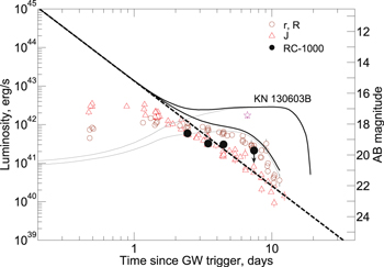
Figure 11. Light curve of the OT in units of stellar magnitudes (right Y-axis) and total luminosity Liso (left Y-axis). Bold black circles represent the observations made by the Chilescope/RC-1000 telescope. Red open triangles and brown open circles show r-, R-, and J-band data, respectively, taken from Villar et al. (2017) and Tanvir at al. (2017). The optical afterglow approximation of GRB 130603B rescaled to the rest frame is shown by the dashed line. The luminosity of a kilonova associated with GRB 130603B is also shown (purple star). The luminosity is calculated from nIR data obtained in the F160W filter of HST (Tanvir et al. 2013). Thin black curves represent the models from Tanvir et al. (2013), corresponding to ejected masses of 10−2 M⊙ [lower] and 10−1 M⊙ [upper] respectively.
Download figure:
Standard image High-resolution imageAppendix B: BSA: Radio Observations at 110 MHz
One of the most sensitive radio telescopes at the frequency of 110 MHz is the Big Scanning Antenna (BSA; Puschino, Russia). BSA is a radio telescope of meridian type. The BSA observation is a continuous survey in multibeam mode in the frequency range of 109.0–111.5 MHz using 96 beams covering a field of view from −8 and up to +42° in decl. with a time resolution of 12.5 ms (Samodurov et al. 2017).
The form of the BSA single beam diagram is described by the function
where x = (π D1/λ) · (α − α0),  , α and δ are equatorial coordinates, (α0, δ0) are the coordinates determining the position of the maximum of the diagram directionality of the radio telescope, D1 = 384 m and D2 = 187 m are the dimensions of BSA in the direction from east to west, and from north to south, respectively, λ = 2.72 m is a wavelength, and Z is the angle between direction to object and antenna normal. It can be found from (38) that the size of the primary beam is about 50 arcmin in R.A. (or nearly 5 minutes) and about 30 arcmin in decl.
The OT position at the time of the GW170817 trigger was 11 5 above horizon at the BSA location, but outside the BSA multibeam diagram, that is, 15° lower in decl. and 4° (or 14 minutes in R.A.) east from the BSA pointing direction. BSA can detect radio transients around twentieth side lobes of southern beams if the transient would be sufficiently bright. It can be found from (38) that the twentieth side lobe has an efficiency of about 3 · 10−4. However, (38) is the formulae for the ideal antenna. Really, bright radio sources such as Sun or Cygnus A (3C 405) are indeed registered in side lobes of BSA at a distance of ±40° with an efficiency of
  and at a distance of ±10° with an efficiency of ∼10−2. As a result, we use side lobe efficiency of 10−2 in our calculation. Details of side lobe BSA calibration can be found elsewhere (V. Samodurov et al. 2018, in preparation).
We investigated all data sets around the GW170817 trigger recorded with BSA. The only significant transient signal with a duration of 1.5 s centered at (UTC) 12:47:44.7 of about 100 Jy was detected in the southern beams at 109.273-111.148 MHz (see Figure 12). We mostly believe the signal has a non-astrophysical nature because of the lack of a dispersion pattern, which is specific for distant astrophysical objects such as, e.g., pulsars. We can place a conservative upper limit of 30 Jy (it is equivalent to S/N > 10) on a timescale of 10–60 s for any astrophysical signal.

Figure 12. BSA observation at 109-110.25 MHz frequency channels (Y-axis) around the GW170817 trigger time (lower X-axis). In particular, in the shown beam toward decl. (J2000) = −4.82 the nearly symmetric signal is visible at frequency channels from 109.898 and up to 110.367 MHz. The signal is visible in the southern beams and centered at (UTC) 12:47:44.7 i.e., 400 s later than the GW170817 trigger time. This is the most powerful signal of about 100 Jy detected during 15 minutes since the GW170817 trigger. It most likely has an artificial origin.
Download figure:
Standard image High-resolution image
We can estimate the intensity of the possible astrophysical signal, which can be detected by side lobes at the time of the GW170817 trigger. The FWHM of the side lobe along R.A. is about 5 minutes. The OT position was 2.5 × FWHM of the diagram at the trigger time of GW170817. Using a projection of the BSA array toward the OT (cos(78.65) = 0.2) and side lobe efficiency ∼10−2, we estimate the upper limit on the transient radio signal from the position of the OT as 15000 Jy. The value can be converted into the upper limit of a luminosity of the radio transient at the distance of the OT  for a duration of the transient in the range of 10–60 s.
Appendix C: SPI-ACS/INTEGRAL Data Analysis
SPI-ACS experiment consisting of 91 BGO crystals is operating in a single energy channel with a lower threshold of ∼80 keV and time resolution of 50 ms (von Kienlin et al. 2003). A script16 was used as the source of input SPI-ACS data.
GRB 170817A was detected in SPI-ACS at a 4.5σ significance level. The burst onset is delayed to GW trigger to ≃2 s. A third-order polynomial model was used to fit the background signal in time intervals (−118, −30) s and (300, 900) s (data before −118 s are not available). We found for GRB 170817A that there is a deviation of SPI-ACS count statistics from Poisson distribution with a factor of ≃1.26 (see, e.g., Minaev et al. 2010a; Minaev & Pozanenko 2017). Statistical uncertainties for SPI-ACS data were estimated, taking into account the factor of deviation.
We found the duration of the burst in SPI-ACS data,  , to be significantly longer comparing with T90 ≃ 0.1 s derived in Savchenko et al. (2017a). Our value is more consistent with GBM results obtained in our paper (see Figure 1 and Section 3.2) and in Goldstein et al. (2017a). The duration,
  , characterizes the burst to be from a short (or type I) population with a probability of ∼74% (see Figure 11 in Minaev & Pozanenko 2017).
The burst fluence calculated for the (2, 3) s time interval since the GW trigger is F = (1.8 ± 0.4) × 103 counts. The off-axis for the GRB 170817A source from the satellite pointing axis is 105 deg, which is quite optimal for detection. In the paper by Viganò & Mereghetti (2009), it was shown that 1 SPI-ACS count corresponds on average to ≈10−10 erg cm−2 in the (75, 1000) keV range, for directions orthogonal to the satellite pointing axis. Using the conversion factor, we derive F = (1.8 ± 0.4) × 10−7 erg cm−2 in the (75, 1000) keV range for GRB 170817A. This value is in agreement with one estimated in Savchenko et al. (2017a) using a more complex method.
We did not find any precursor or extended emission components in SPI-ACS data at timescales from 0.05 up to 100 s in the time interval (−50, 200) s since the GW trigger, and we estimated upper limits on their intensity. At a timescale of 0.05 s, the upper limit on precursor activity is Sprec ≃ 250 counts or Sprec ≃ 2.5 × 10⁻⁸ erg cm−2 at a 3σ significance level. At a timescale of 50 s, the upper limit on extended emission activity is SEE ≃ 8100 counts or SEE ≃ 8.1 ×10⁻⁷ erg cm−2 at the 3σ significance level.
Assuming redshift z = 0.00968 and luminosity distance DL =42.0 Mpc for the source (Jones et al. 2009), we estimated total isotropic energy release in the energy range (75, 1000) keV as Eiso = (3.9 ± 0.9) × 1046 erg. One can estimate the upper limits on the precursor and extended emission component expressed as total isotropic energy release as well:  and
and  , correspondingly.
Appendix D: Magnetic Force-free Bomb
At the moment of the breakout, the jet, which was strongly magnetically dominated close to the BH but became mildly magnetically dominated during the confined propagation (Section 4.1), starts to expand and accelerate. As the pair density falls precipitously, the flow becomes more and more magnetically dominated. In this appendix, we consider the explanation of a magnetic force-free bomb—radial motion of the post-breakout highly magnetized plasma flows.
Consider the radial expansion of force-free plasma carrying the toroidal magnetic field. The relativistic force-free condition implies that the total EM force vanishes (Gruzinov 1999)
(for the GR formulation, see Komissarov 2011; Lyutikov 2011c).
Separating the angular and the time-radial dependence, Bϕ = Bϕ(t, r) bϕ (θ) and  , we find two types of solutions. The first is the solution self-similar in Z = r/t,
Equation (40) represents solutions for the polar-angle-dependent expansion of force-free plasma into vacuum. Poynting flux is zero at the edge of the outflow at r = t and increases for smaller r. If the source is located at r ≪ t, it is required that the source luminosity increases with time ∝t2 for the solution to be applicable.
Second, looking for a solution of the type Bϕ, Eθ ∝ 1/r, we find that the following scaling satisfies the Maxwell equations

where f is an arbitrary function of the argument. This solution represents a force-free pulse of initial shape f(r), moving with the speed of light—a force-free bomb.
Both solutions (40) and (41) are different from EM fields in vacuum since there are non-zero currents and charge densities in the flow. A general time-dependent approach to force-free fields for the specific case of ρ = j has been discussed by Gralla & Jacobson (2014); see Lyutikov (2011b) for a related time-dependent solution in general relativity.
Footnotes
- 9
- 10
- 11
- 12
- 13
- 14
- 15
- 16