


Abstract
Electrons are accelerated to non-thermal energies at shocks in space and astrophysical environments. While different mechanisms of electron acceleration have been proposed, it remains unclear how non-thermal electrons are produced out of the thermal plasma pool. Here, we report in situ evidence of pitch-angle scattering of non-thermal electrons by whistler waves at Earth's bow shock. On 2015 November 4, the Magnetospheric Multiscale (MMS) mission crossed the bow shock with an Alfvén Mach number ∼11 and a shock angle ∼84°. In the ramp and overshoot regions, MMS revealed bursty enhancements of non-thermal (0.5–2 keV) electron flux, correlated with high-frequency (0.2–0.4  , where
  is the cyclotron frequency) parallel-propagating whistler waves. The electron velocity distribution (measured at 30 ms cadence) showed an enhanced gradient of phase-space density at and around the region where the electron velocity component parallel to the magnetic field matched the resonant energy inferred from the wave frequency range. The flux of 0.5 keV electrons (measured at 1 ms cadence) showed fluctuations with the same frequency. These features indicate that non-thermal electrons were pitch-angle scattered by cyclotron resonance with the high-frequency whistler waves. However, the precise role of the pitch-angle scattering by the higher-frequency whistler waves and possible nonlinear effects in the electron acceleration process remains unclear.
Export citation and abstract BibTeX RIS
1. Introduction
In the "diffusive shock acceleration" scenario of cosmic rays (e.g., Axford 1977; Bell 1978; Blandford & Ostriker 1978), electrons need to be sufficiently energetic before being injected into the process. The problem of how non-thermal electrons are first produced out of thermal plasma pool is termed the "injection problem" and has long been a subject of debate (e.g., Levinson 1992; Amano & Hoshino 2010).
In space plasmas, in situ measurements are available seamlessly from thermal to non-thermal energy ranges. At and around the transition layer of Earth's bow shock and interplanetary shocks, a "spiky" enhancement of energetic electrons (typically up to 100 keV) has been detected in particular when the shock angle  (the angle between the shock-normal direction and the upstream magnetic field) is large (e.g., Fan et al. 1964; Anderson 1969; Tsurutani & Lin 1985; Gosling et al. 1989). These observations have been interpreted in the framework of shock drift acceleration at magnetic gradients (e.g., Sarris & van Allen 1974; Chen & Armstrong 1975; Leroy & Mangeney 1984; Wu 1984).
Whistler waves have also been suggested to play an important role for electron acceleration at shocks (e.g., Shimada et al. 1998; Oka et al. 2006, 2009; Riquelme & Spitkovsky 2011; Wilson et al. 2012; Matsukiyo & Matsumoto 2015; Masters et al. 2016). In the shock transition layer, oblique whistler waves are often found in the frequency range below the lower-hybrid frequency (e.g., Rodriguez & Gurnett 1975; Wilson 2016). In addition, higher-frequency (typically 0.1–0.5  where
where  is the cyclotron frequency), parallel-propagating whistler waves have also been detected (e.g., Zhang et al. 1999; Hull et al. 2012).
In this Letter, we report direct evidence of cyclotron resonance between non-thermal electrons and the high-frequency whistler waves during a crossing of Earth's bow shock by NASA's four-spacecraft mission, Magnetospheric Multiscale (MMS).
2. Observation
On 2015 November 4, all four MMS spacecraft crossed the bow shock at around 04:58 UT from the upstream (solar wind) side near the subsolar point (Figure 1(a)). The upstream Alfvén Mach number and the shock angle are estimated to be  and
and  , respectively. Here, MA is estimated in the shock-rest, shock-normal incidence frame, and the shock-normal vector
  ∼ (0.998, 0.049, −0.025) is estimated using a semi-empirical global model (Peredo et al. 1995). We confirmed that the ion velocity data were consistent with that of the OMNI data (after a time adjustment) obtained by the ACE spacecraft at L1 with up to a few percent differences. Then, we confirmed that the minimum variance analysis, timing analysis, and the Rankine–Hugoniot based method yielded consistent results (see Paschmann & Daly 1998 for the techniques and analysis). The shock speed relative to the spacecraft is estimated to be ∼21 km s−1. The spacecraft potential (3–5 V) had little effect on the >100 eV electrons presented in this Letter. The upstream magnetic field was
  ∼ (−0.38, −8.1, 0.24) nT as illustrated in Figure 1(a) (green arrows). The Geocentric Solar Ecliptic coordinate is used throughout this Letter unless otherwise noted. All four spacecraft observed similar features due to the small inter-spacecraft distance of ∼20 km (or ∼10
  , where
  is the electron inertia length, and the upstream electron density
  cm−3 is used).
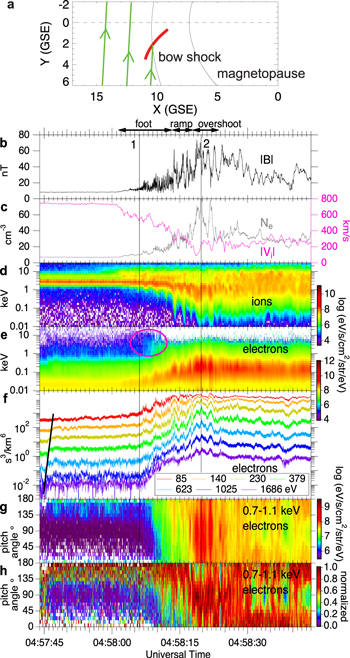
Figure 1. Overview of the shock crossing on 2015 November 4 by MMS. (a) Spacecraft trajectory (red curve) and the configuration of the bow shock (black curve), (b) magnetic field magnitude, (c) electron density and ion flow speed, ((d), (e)) ion and electron spectrograms, (f) electron phase-space densities, (g) pitch-angle distribution of 0.7–1 keV electrons, and (h) same as (g), but normalized at each time bin. The boundary models are scaled to match the location of the shock crossing.
Download figure:
Standard image High-resolution imageFigures 1(b)–(h) show selected plasma parameters, providing an overview of the shock crossing. At 04:57:45 UT, MMS3 moved from the pristine solar wind into the electron foreshock in which the interplanetary magnetic field is connected to the bow shock, as indicated by the energy-dispersed flux enhancement (diagonal black line in Figure 1(f)). Then, MMS3 entered into the shock transition layer at around 04:58:02 UT, as evidenced by the gradual increase and decrease of the magnetic field magnitude (Figure 1(b)) and the solar wind speed (Figure 1(c)), respectively. These parameters leveled off in the downstream region (after around 04:58:33 UT). During the shock crossing, MMS3 observed a burst of higher-energy (>2 keV) electrons at around 04:58:10 UT, highlighted by the pink circle in Figure 1(e). However, the counting statistics were low in this energy range (due to the limited sensitivity of the detectors). Also, the angular information of electrons in this energy range (> 2 keV) was lost for data after 04:58:10 UT due to irreversible data compression (Barrie et al. 2017). Thus, in this Letter, we focus only on an intermediate energy range of 0.5–2 keV, which is, as will be shown later, marginally non-thermal.
The phase-space density of these moderately energetic electrons showed an exponential increase between 04:58:06 UT and 04:58:20 UT (Figure 1, vertical lines 1 and 2, respectively). Unlike the entry into the foreshock, the increase started simultaneously in all energy channels, indicating that the spacecraft entered into a region where electrons are accelerated and confined. The pitch-angle range was broad (Figures 1(g), (h)), corroborating our interpretation of electron confinement. We emphasize that the increase was not smooth and accompanied by shorter-timescale, bursty enhancements, indicating that there were smaller-scale processes at work.
To investigate the shorter-timescale variations of the energetic electrons, we examined various plasma parameters around the ramp and overshoot regions (Figure 2). We found that the energetic electron enhancements occurred quasi-periodically (Figure 2(d)) in the direction perpendicular to the local magnetic field direction, i.e., pitch angle ∼90° (Figure 2(c)). These features indicate that the non-thermal electrons were confined and/or accelerated locally.
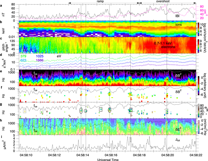
Figure 2. Plasma parameters around the ramp and overshoot regions, demonstrating correlated and quasi-periodic bursts of energetic electron flux and whistler waves. (a) Magnetic field magnitude  and electron density Ne, (b) ion spectrogram, (c) pitch-angle distribution of 0.7–1.1 keV electrons, (d) electron phase-space density, (e) magnetic power spectral densities, (f) same as (e), but extracted data points that satisfy the whistler wave criteria (see the text), (g) whistler wave propagation direction with 180° ambiguity, (h) power spectral densities of the electric field y-component in the DSL coordinate, and (i) total current estimated from plasma moment data. In panel (g), the circles and rectangles indicate propagation toward upstream and downstream, respectively. The thick circles and rectangles indicate there was an enhanced shoulder feature in the electron distribution. In panels (e)–(h), the black and white curves show the electron cyclotron frequency
  .
.
Download figure:
Standard image High-resolution imageThe electron bursts were associated with the broadening of the yellow–green region toward lower energies in the ion energy spectrogram (Figure 2(b)), indicating that the quasi-periodic occurrence of the electron bursts were related to ion dynamics. In fact, the time intervals between these bursts were roughly 2 s, comparable to the ion gyro-period  for
for  nT or ∼3.3 s for
  nT. Thus, we attribute this quasi-periodicity to non-stationarity (reformation; e.g., Leroy et al. 1982; Lembège 2002) and/or non-uniformity (ripples; e.g., Lembège 2002; Lowe & Burgess 2003; Johlander et al. 2016).
It appears that the energetic electron bursts were not necessarily associated with enhancements of magnetic field magnitude/gradients (Figure 2(a)). Here, we use the total current  as a proxy of magnetic spatial gradients because of Ampére's law (
 ). Figure 2(i) shows
  estimated from the plasma moment data. It is evident that some of the electron bursts (especially those highlighted by the first, third, and fifth vertical lines) were not correlated with the current enhancements (and hence magnetic gradients). We also estimated the current from the magnetic field measured by all four spacecraft via Ampére's law (
 ), but the result was not consistent with the current estimated from plasma moment, indicating that ∇ × B was not uniform over the spatial scale of the inter-spacecraft distance, 20 km (or 15–25
  using
using  ).
).
Figures 2(e)–(g) show that some (but not all of the) electron bursts were correlated with higher frequency (i.e., 200–400 Hz; 0.2–0.4  , where
  is the electron cyclotron frequency), parallel-propagating (
 ) whistler waves (as highlighted by the vertical lines). While the magnetic field fluctuations contained both transverse and compressional components (Figure 2(e)), we extracted data points with clear signatures of right-hand polarized whistler waves (in the spacecraft frame). Figure 2(f) only shows data points with the degree of polarization greater than a noise level of 0.7 and the ellipticity greater than 0.5, where ellipticity is the ratio (minor axis)/(major axis) of the ellipse transcribed by the field variations of the components transverse to the background magnetic field (Samson & Olson 1980). Then, we calculated the wave normal angle
  between the magnetic field direction and the wave
  -vector with the plane wave assumption (Means 1972), which still contains the 180° ambiguity (Figure 2(g)). Here, we emphasize that the similar, higher-frequency whistler waves were detected not only in the ramp region but also in the foot, overshoot, and downstream regions. The frequency range, obliquity, and the periodic nature of the higher-frequency whistler waves are consistent with earlier studies of the bow shock transition layer (e.g., Zhang et al. 1999; Hull et al. 2012).
As an independent approach of characterizing the waves, we used the minimum variance analysis of bandpass filtered data, combined with electric field data via the Faraday's law (e.g., Hull et al. 2012). Such an analysis allows us to estimate the wave k-vector without the 180° ambiguity. In Figure 2(g), the sign of the k-vectors with respect to the magnetic field direction is indicated by open circles for negative or propagation toward upstream and open rectangles for positive or propagation toward downstream. While some whistler bursts were directed toward downstream, some other bursts of higher-frequency whistler waves were directed toward upstream.
Figure 3 shows an example of the waveform analysis with the Faraday's law, taken from the burst at 04:58:13.9 UT (the first vertical line in Figure 2). Figures 3(b), (c) show the original (i.e., unfiltered) waveform of the magnetic and electric fields. Figure 3(d) shows the frequency ( )–wavenumber (
 ) diagram in the plasma rest-frame after Doppler-shift correction, where
  ,
,  ,
,  is the electron cyclotron frequency and
  is the electron plasma frequency. We confirmed that the estimated values of
  ∼ 0.6–0.8 are consistent with those estimated by a conventional approach of assuming the cold plasma dispersion relation for whistler waves (instead of using electric field data; e.g., Coroniti et al. 1982; Wilson et al. 2013). The estimated values of
  indicate that the waves satisfied the Landau resonance condition with <20 eV electrons only. On the other hand, the waves (especially those indicated by red points in Figure 3(d)) satisfied the cyclotron resonance condition with 100–400 eV electrons.

Figure 3. Waveforms and characteristics of the higher-frequency parallel-propagating whistler waves in the burst of 04:58:13.9 UT. From top to bottom are (a) magnetic field magnitude from the fluxgate magnetometer (FGM; Russell et al. 2014), (b) unfiltered magnetic field vector from the search-coil magnetometer (SCM; Le Contel et al. 2016), (c) electric field vector from Spin-plane Double Probes (SDP; Lindqvist et al. 2016) and Axial Double Probes (Ergun et al. 2016), and (d) the dispersion in the plasma rest-frame. In panel (d), each data point has a different value of estimated  (not shown). For reference, the black curves show cold plasma approximation for whistler waves with different values of
  .
.
Download figure:
Standard image High-resolution imageTo understand how electrons behaved during the wave burst, we examined electron velocity distribution as measured by the Fast Plasma Instrument (FPI; 30 ms sampling; Pollock et al. 2016) and the Electron Drift Instrument (EDI; 1 ms sampling; Torbert et al. 2016). The primary purpose of EDI is to determine the ambient electric field from calculations of the electron drift velocity by emitting two weak beams of electrons from opposite sides of a spacecraft and recapturing them after one or more gyrations. However, the beam detector can alternatively be used to measure ambient electrons at high time resolution (1 ms) with a limited field of view and angular and energy resolution.
Figures 4(a), (b) show the magnetic field waveform and its dynamic spectra during the burst, indicating that the whistler waves were peaked around 200–250 Hz. Figures 4(c)–(l) show the time profiles and their dynamic spectra of EDI electron fluxes. EDI has a total of eight channels (i.e., look directions), and on this day, they were measuring 0.5 keV electrons that were either roughly parallel or anti-parallel to the local magnetic field, as indicated by the labels in Figures 4(e)–(l). The dynamic spectrum of Channel 4 (with its direction varied in the 25°–40° pitch-angle range) showed the most intense fluctuation of the electron flux at 200–250 Hz. There was a similar but weaker signal in Channels 2 and 3 (with smaller pitch angles). The match of the timing and frequency between the electron flux fluctuation and the high-frequency whistler waves indicates that the non-thermal electrons at 0.5 keV were interacting with the whistler waves.
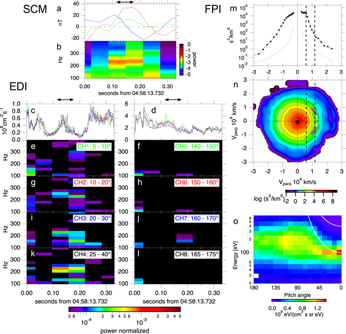
Figure 4. Electron and magnetic field data during the burst at ∼04:58:13.9 UT, demonstrating evidence of electron pitch-angle scattering by cyclotron resonance with whistler waves. (a) The waveforms and (b) dynamic spectra of the magnetic field vectors. (c) The fluxes of 0.5 keV electrons measured at four different pitch-angle ranges (but roughly parallel to the magnetic field) indicated by different colors and corresponding labels in panels (e), (g), (i), and (k). (d) Same as (c), but for the channels that were roughly anti-parallel to the magnetic field. ((e)–(l)) The dynamic spectra of the 0.5 keV electron fluxes dF2, normalized by the intensity F2. The electron distribution function at 2015-11-04/04:58:13.8478-13.9078 (as indicated by the horizontal arrows above panels (a), (c), and (d)) in (m) 1D velocity space, (n) 2D velocity space, and (o) energy pitch-angle space. In panel (m), all data points with pitch angles 0°–25° and 155°–180° are used from the full 3D velocity distribution. In panel (n), a slice along the plane perpendicular to the magnetic field B and the electron bulk velocity  is taken from the full 3D but interpolated velocity distribution. In panel (o), all data in the full 3D velocity space are used. The vertical dashed lines in panels (m) and (n) and the curved lines in panel (o) represent the resonance energies inferred from the waveform analysis in Figure 3. The pink (gray) curves show the positions of the look direction of the EDI data in panel (k) (other panels).
Download figure:
Standard image High-resolution imageFigures 4(m), (n) show the electron velocity distribution as measured by FPI during the wave burst. The positions of the EDI look directions in the velocity space are indicated by the gray and pink curves in Figure 4(n). The pink curves indicate the positions of the 25°–40° channel, which recorded the strongest signal at 200–250 Hz. The positions of the pink curves (when projected to the horizontal axis) match roughly with the resonant energies of  eV (the vertical dashed lines), which were derived independently from the waveform analysis in Figure 3, indicating that the interaction between the 0.5 keV electrons and the whistler waves was due to cyclotron resonance. In fact, the velocity distribution function exhibits an enhanced gradient of phase-space density in the resonant energy range (Figures 4(m), (n)), which may be interpreted as a source of the whistler waves.
Figure 4(o) provides another view of the electron distribution in the energy versus pitch-angle space. The color code indicates energy flux instead of phase-space density. The enhanced gradient of the phase-space density can now be seen as the gradient of the energy flux in the region bounded by the white curves of  .
.
Figure 4(o) also indicates that there were two populations that could have been involved in the phase-space density gradient and the generation of the high-frequency whistler waves. The first population was found around ∼100 eV near 0° pitch angle (red and yellow in Figure 4(o)). This is seen as the shoulder around  ∼ 6000 km s−1 in Figure 4(m) and is embedded in the red region in Figure 4(n). Such features remind us of earlier studies that reported a parallel electron beam superposed on a flat-top core component (e.g., Feldman et al. 1982). The second population is in the 100–400 eV range centered around 90° pitch angle. A numerical approach may be necessary to pin down the precise source of whistler wave generation (e.g., Tokar et al. 1984; Veltri & Zimbardo 1993), which is beyond the scope of this Letter.
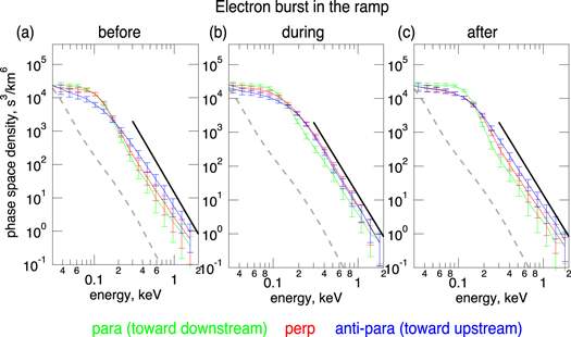
Here, we examine whether the 0.5 keV electrons as seen in the EDI data were in the non-thermal energy range or not. Figure 5 shows the electron energy spectrum before, during, and after the burst at 04:58:13.9 UT. Here, we took an average over 120 ms (four samplings), roughly equal to the duration of the wave burst, because all four samplings showed similar features.
Figure 5. Evolution of the electron energy spectrum around the electron burst at 04:58:13.9 UT. Each spectrum is a 120 ms (four sampling) average starting from (a) 04:58:13.6078 UT, (b) 04:58:13.8178 UT, and (c) 04:58:13.9978 UT, obtained in the pitch-angle ranges of 0°–45° (green; parallel direction), 45°–135° (red; perpendicular direction), and 135°–180° (blue; anti-parallel direction). The gray dashed curve is the omni-directional spectrum in the pristine solar wind (04:57:40–04:57:45 UT). The black solid line is a reference to a slope of 4.10, which was obtained by fitting the perpendicular spectrum obtained during the burst.
Download figure:
Standard image High-resolution image
It is evident that the perpendicular component (red curve) was enhanced during the burst, consistent with what we saw in pitch-angle distributions (Figures 2(c) and 4(o)). The energy spectra show that, during the burst, the phase-space density of the perpendicular component became comparable to that of the anti-parallel component (blue curve). Also, a power-law form is visible above ∼300 eV and extends up to at least 2 keV. While the energy range spans a little less than an order of magnitude, we confirmed that the spectrum in this energy range (300–2000 eV) is not fitted well with a Maxwellian distribution. We also confirmed that the entire spectrum (from 40 to 2000 eV) is not well fitted with the kappa distribution.
3. Summary and Discussion
The electron-scale measurements by MMS revealed quasi-periodic and correlated bursts of energetic electron flux and high-frequency whistler waves in the ramp and overshoot regions of the bow shock transition layer. The electron signatures (a phase-space density gradient in the FPI data and a flux variation at the same frequency in the EDI data) constitute an evidence of pitch-angle scattering of non-thermal electrons by the high-frequency whistler waves via cyclotron resonance.
However, it remains unclear how the pitch-angle scattering via cyclotron resonance contributed to the electron acceleration process during the correlated bursts of non-thermal electrons and high-frequency whistler waves. In the framework of quasi-linear theory, electromagnetic waves propagating in the opposite directions are needed to energize particles in the perpendicular direction. However, the high-frequency whistler waves were propagating in one direction in each wave burst, although different bursts had different directions of wave propagation (circles and rectangles in Figure 2(g)). While the wave amplitude was small ( ), there could have been nonlinear effects.
We also note that the peaks of electron phase-space densities were not always associated with whistler waves (see the peaks without vertical lines in Figure 2). In the foot region, where we saw the initial rise of the phase-space density of energetic electrons (Figure 1(f)), large amplitude ( ) magnetic field fluctuations were dominant. All these features suggest there could be an electron acceleration process that does not involve cyclotron resonance with the high-frequency whistler waves.
The appearance of quasi-periodic and correlated bursts of non-thermal electrons and high-frequency whistler waves is attributed to non-stationarity and/or non-uniformity of the shock front. This is because the bursts were also correlated with ion dynamics including the ion-scale magnetic field fluctuations (see Lembège 2002 for a similar argument). More sophisticated models/simulations may be necessary to understand the appearance of the high-frequency waves and the precise role of the cyclotron resonance in the entire process of electron acceleration at the bow shock.
We thank all members of the MMS project. We acknowledge use of OMNI data provided by Space Physics Data Facility at NASA/GSFC. We also acknowledge NASA grants NNG04EB99C (SwRI) and NNX08AO83G (UC Berkeley). The French involvement (SCM instruments) is supported by CNES, CNRS-INSIS, and CNRS-INSU.