


Abstract
Coronal mass ejections (CMEs) are the largest and most dynamic explosions detected in the million degree solar corona, with speeds reaching up to 3000 km s−1 at Earth's orbit. Triggered by the eruption of prominences, in most cases, one of the outstanding questions pertaining to the dynamic CME-prominence system is the fate of the cool  ejected filaments. We present spectroscopic observations acquired during the 2015 March 20 total solar eclipse, which captured a plethora of redshifted plasmoids from Fe xiv emission at
  . Approximately 10% of these plasmoids enshrouded the same neutral and singly ionized plasma below
  , observed in prominences anchored at the Sun at that time. This discovery was enabled by the novel design of a dual-channel spectrometer and the exceptionally clear sky conditions on the island of Svalbard during totality. The Doppler redshifts corresponded to speeds ranging from under 100 to over 1500 km s−1. These are the first comprehensive spectroscopic observations to unambiguously detect a
  filamentary CME front with inclusions of cool prominence material. The CME front covered a projected area of
  starting from the solar surface. These observations imply that cool prominence inclusions within a CME front maintain their ionic composition during expansion away from the Sun.
Export citation and abstract BibTeX RIS
1. Introduction
Prominences are considered to be one of the visual highlights of a total solar eclipse, with their characteristic bright red color due to Hα emission and their complex dense structures lying low in the corona. Prior to space-based measurements, catalogs of eruptive prominences produced from Hα observations showed that their speeds increased with heights to a maximum recorded value of 1280 km s−1 at a heliocentric distance of 3 Rs (Kleczek 1964). (All distances given in this Letter are heliocentric.) In addition to Hα, emission from prominences is characteristic of neutrals and singly or doubly ionized elements, typical of  chromospheric material (Tandberg-Hanssen 1995). Their ionization state is in stark contrast to that of the surrounding highly ionized coronal plasma at temperatures of a few 106 K. Furthermore, multi-wavelength eclipse observations have amply demonstrated that prominences are found to be always enshrouded by
  plasma in the corona (Habbal et al. 2010b).
With the advent of space-based observations, the occasional disruption of prominences was found to trigger gigantic eruptions in the overlying coronal material, in the form of bubble- or tornado-shaped fronts, known as coronal mass ejections (CMEs). The erupting prominences invariably formed their bright core (House et al. 1981; Illing & Hundhausen 1985; Gopalswamy et al. 2003; Chen 2011). Reported CME speeds, of a few hundred to 2000 km s−1 within a few Rs (Yashiro et al. 2004; Yurchyshyn et al. 2005), were comparable to the earlier reported speeds of eruptive prominences (Kleczek 1964). Recently, Howard (2015a, 2015b) and Wood et al. (2016) found a few "rare" examples of very bright CME-associated prominences that were imaged out to 1 au with the heliospheric imagers on the two Solar Terrestrial Relations Observatory (STEREO) spacecraft (Kaiser et al. 2008).
The lack of spectroscopic capability in these coronagraphic data, however, is such that no information regarding the electronic and ionic temperature of CMEs, and the changes, if any, in the ionization state of any accompanying prominence material can be obtained. The first observations to yield any thermodynamic information were those from the extreme-ultraviolet spectroheliometer on the Apollo Telescope Mount on Skylab in the early 1970s (Reeves et al. 1977). Schmahl & Hildner (1977) reported an eruptive event whereby 10% of the filamentary prominence material maintained a temperature of  as it rose in the corona up to the 3 Rs limit of the field of view. The next opportunity materialized with the Ultraviolet Coronagraph Spectrometer (UVCS) on SOHO (Kohl et al. 1995). Since the lowest slit position of the spectrometer was at 1.5 Rs, these observations were often combined with contemporaneous extreme-ultraviolet observations, primarily from SOHO/EIT, to follow the origin and dynamics of an eruptive prominence–CME system starting from the solar surface outward. The main result to emerge from these studies was the helical nature of strands at temperatures ranging from
  to
to  , lending evidence for the survival of some chromospheric prominence material out to a few Rs (Ciaravella et al. 1997, 2000; Akmal et al. 2001; Raymond 2002; Raymond & Ciaravella 2004; Landi et al. 2010; Giordano et al. 2013; Lee & Raymond 2014).
The survival of a fraction of cool prominence material with its expansion into interplanetary space was demonstrated by in situ measurements. The most compelling evidence was the detection of enhanced singly ionized He (He+; Gosling et al. 1980), and unusually low charge states, e.g., O5+, Fe5+ (Burlaga et al. 1998); O3+, N3+, C2+ (Gloeckler et al. 1999); C2+, O2+, Fe4+ (Lepri & Zurbuchen 2010). These low charge states were found to be contemporaneous with measurements of high charge states of the multi-million degree CME plasma and have thus been interpreted as remnants of prominence material.
In this Letter, we report on the first comprehensive spectral observations obtained during the total solar eclipse of 2015 March 20, which led to the serendipitous discovery of a large number of spatially discrete Doppler-shifted fragments of Fe xiv 530.3 nm (i.e., Fe+13 ions) emission, scattered across a projected area of 2.5  in the plane of the sky off the east limb of the Sun, with speeds ranging from under 100 to over 1500 km s−1. Embedded within approximately 10% of them was Doppler-shifted emission from neutrals and singly ionized elements of Cr, He, Fe, and Mg. These observations are interpreted as evidence of filaments forming a large
  CME front, enshrouding filaments of cool prominence material that had preserved its original ionic composition.
2. Spectrometer Design and Operation
To capture the spectral composition of coronal structures, a dual-channel partially multiplexed two-dimensional imaging spectrometer (PaMIS) was designed and built for eclipse observations (see Figure 1). The two channels were centered on the Fe xi 789.2 nm and Fe xiv 530.3 nm lines, each with a 70 nm bandpass, separated by specially designed bandpass filters. The choice of these spectral lines was based on earlier multi-wavelength eclipse observations that showed that coronal structures were essentially dominated by two (electron) temperature regimes  and
and  , corresponding to the peak ionization temperatures of Fe xi and Fe xiv, respectively (Habbal et al. 2010a).
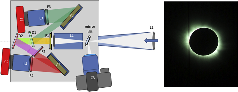
Figure 1. Schematic design of the dual-channel spectrometer. Channel 1 is centered on Fe xiv 530.3 nm, and channel 2 on Fe xi 789.2 nm. The main components of the spectrometer consist of two echelle gratings (G1 and G2), a combination of multi-layer dichroic mirrors (D1, D2), and multi-layer coated color glass filters (F1, F2, F3, and F4), which limited the bandpass of each channel to approximately 70 nm. The spectra in each channel were recorded on two Atik314L cameras (C1 and C2), each with a detector size of 1000 (spatial) × 1400 (spectral) 6.5 μm pixels. The entrance slit position together with the image of the corona were captured by the reflective mirror slit onto camera C3, as shown on the right. L1 is a Zeiss telephoto lens (Sonar F/4, f = 300 mm). L2 is a projection lens (ASKINAR F/1.9, f = 100 mm), and L3 and L4 are refocusing lenses. The physical size of the spectrometer is 10'' × 14'' × 20''.
Download figure:
Standard image High-resolution imageThe entrance slit of the spectrometer was produced by laser ablation of a 30 μm × 2 cm rectangular part from an Al-coated mirror. The rest of the mirror surface reflected the image of the corona onto a video camera, such that the position of the slit, relative to the Moon-occulted Sun, could be monitored as a function of time. The optical design was such that the Sun diameter covered 25% of the usable 8 Rs length of the slit.
As the resolution of such an instrument is proportional to the grating order and inversely proportional to the slit width, PaMIS was operated in high (approximately 40th) order. The limited bandpass of 70 nm in each of the two channels enabled a relatively easy disentanglement of the overlapping orders.
The fact that several orders were recorded at each slit position during its operation yielded a valuable reference to check against any artifacts. For example, while He i in 37th order overlapped Fe xiv in 41st order, they were separated in the He i 38th order and the Fe xiv 42nd order. Furthermore, a small transmission beyond the long wavelength end enabled the detection of very strong lines such as He i 587.6 nm in the Fe xiv 530.3 nm channel and Fe xiii 1074.7 nm in the Fe xi 789.2 nm channel.
Using an effective slit width of 30 μm, a wavelength resolution,  , enabled the recording of the (non-relativistic) Doppler shift
  , of an emission line at wavelength λ, with a velocity accuracy along the line of sight of
  (where c is the speed of light).
3. Observations
The spectroscopic observations presented here were acquired during the total solar eclipse of 2015 March 20, from the old Auroral Station in Adventdalen, operated by the University Centre in Svalbard (UNIS), about 10 km away from the small town of Longyearbyen on the island of Svalbard, Norway. The coordinates were N 78°12' 09 1, E 15° 49' 445 at an altitude of 15 m. Totality, or second contact, started at 10:10:47 UT and ended at third contact at 10:13:14 UT, thus lasting 2 minutes 27 s.
Starting near central meridian at the beginning of totality, the motion of the tracking mount was disabled. The Sun thus drifted across the field of view, enabling the slit of the spectrometer to scan the corona eastward across a distance of 2.5 Rs throughout its 2.5 minute duration of totality. The download time from the detector was 2 s, thus extending the time difference between adjacent exposures. The exposure time at each slit position, starting at position 346 (1st position, almost at central meridian) to 383, was 1 s (or effectively 3 s including download time), yielding a spatial resolution of 45 arcsec. The exposure time was then increased to 2 s (or effectively 4 s) for the remainder of the time, when 14 spectra (slit positions 384–397) were obtained with a spatial resolution of 60 arcsec.
Emission from any spectral line, within the 70 nm bandpass of the Fe xiv channel, was detected in at least two orders, as shown in the example of Figure 2. Calibration of this channel was achieved by using the 532.6 nm emission from a doubled Nd:YAG laser, as well as a Fraunhofer absorption spectrum of the solar disk. The low number (approximately 30) of emission lines present in each channel facilitated their wavelength assignment.
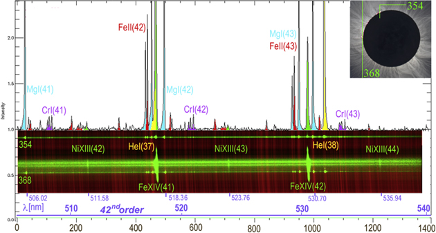
Figure 2. Overlay of two coronal emission spectra (green) onto an inverted Fraunhofer absorption spectrum (red) of the background sky, in the Fe xiv channel. The spectra correspond to slit positions 354 and 368, whose positions are shown in the upper right hand corner, as imaged onto the white-light eclipse image. The slits intercepted prominences, one at the northeast, and the other near the equator. The line plot corresponds to the spectrum at position 354. The spectral orders are shown in brackets: e.g., 42nd and 43rd orders for Fe xiv and 42nd, 43rd, and 44th orders for Ni xiii (green). Emission from elements in low ionization states, such as Mg i (blue) and Cr i (violet) in orders 41, 42, and 43; He i (yellow) in orders 37 and 38; and Fe ii (red) in orders 42 and 43, was recorded at both slit positions. Weaker Fe i emission lines (red) were also detected. The wavelength scale for the 42nd order is given at the bottom. The scale for other orders can be calculated from this wavelength scale.
Download figure:
Standard image High-resolution imageThe fortuitous presence of prominences at the solar limb, when intercepted by the slit, and the fortuitous presence of chromospheric emission lines within the bandpass of both channels, served as an invaluable wavelength reference for any chromospheric emission in the corona. As shown in Figure 2, for two such slit positions, 354 and 368, the overlay of the coronal emission spectrum with the Fraunhofer absorption spectrum matched perfectly: the very narrow Cr i and Mg i triplets and Fe ii lines, and other weaker Fe i lines (not labeled), characteristic of chromospheric emission, could thus be readily identified in emission from the corona and absorption in the Fraunhofer sky spectrum. The coronal emission lines of Fe xiv 530.3 nm and Ni xiii 511.58 nm, not present in the Fraunhofer absorption spectrum, were identified by their larger spatial extent along the slit.
The spectral order number, n, of a line was—to first approximation—obtained by counting the orders of the spectrum of a green laser 532 nm line, starting from order 0 (reflection) to the order of maximum intensity. Accurate determination of the grating order was then achieved by comparing the apparent position of the Fe xiv line in relation to the position of the chromospheric Fe ii and Mg i triplet lines (λ = 516.9, 516.7, 517.3, 518.4 nm), taking into account the different order number. (Lines with reduced wavelength  /n, show up at the same pixel position.) Only the assignment of 41st (left), 42nd (middle), and 43rd (right) order to the Cr and Mg triplet lines and 42nd (middle) and 43rd order (right) to Fe xiv gave the correct position of the emission lines with respect to each other.
In the Fe xi channel, emission from an O i triplet at 777.19, 777.42, and 777.54 nm also appeared at the two slit positions that intercepted the prominences at the limb. In their vicinity, the Fe xi intensity dropped significantly, while emission from Fe xiii 1074.7 nm appeared. This is identical to what had been observed in earlier multi-wavelength eclipse images (see Habbal et al. 2010b). A similar calibration procedure was followed for the Fe xi channel using the position of the O i triplet in relation to those of Fe xi and Fe xiii. Unfortunately, the choice of exposure times for the Fe xi channel proved to be too short to acquire meaningful data past 1.2 Rs because of the low quantum efficiency of the detector at that wavelength. In what follows, the results will therefore pertain only to the Fe xiv channel.
4. Results
Shown in Figure 3 are examples of spectra taken in the Fe xiv channel at three different slit positions, 354 (A) when part of the slit intercepted the occulted solar disk, 378 (B) at 1.4 Rs, and 395 (C) at 2.3 Rs. The slit position in each panel is indicated by a dashed white line, with its position overlaying the corresponding white-light image of the corona taken during totality by M. Druckmüller, and processed by him, to highlight the finest details of coronal structures. To the left of the slit is the two-dimensional spectrum in 42nd order for Fe xiv. As noted earlier, and as can be clearly seen here, slit position 354 (A) intercepted a prominence at the limb, where emission from neutral Fe i, He i, and the Mg i and Cr i triplets was detected, in addition to a ubiquitous background Fe xiv emission. (Note that the overlaid spectrum in panel (A) has been shifted slightly from the slit position (dashed line), so as to expose the intercepted prominence.) Further out in the corona, such as in positions 378 (B) and 395 (C), Doppler redshifts appeared in Fe xiv in some sections along the slit. These sections will be referred to as plasmoids in what follows. They appeared superimposed on the white-light emission caused by electron scattering shown by the white bands in Figure 3. Some of these Fe xiv Doppler-shifted plasmoids were accompanied by He i, Fe ii, and Mg i triplet emission, indicative of the presence of chromospheric material from prominences embedded within them.
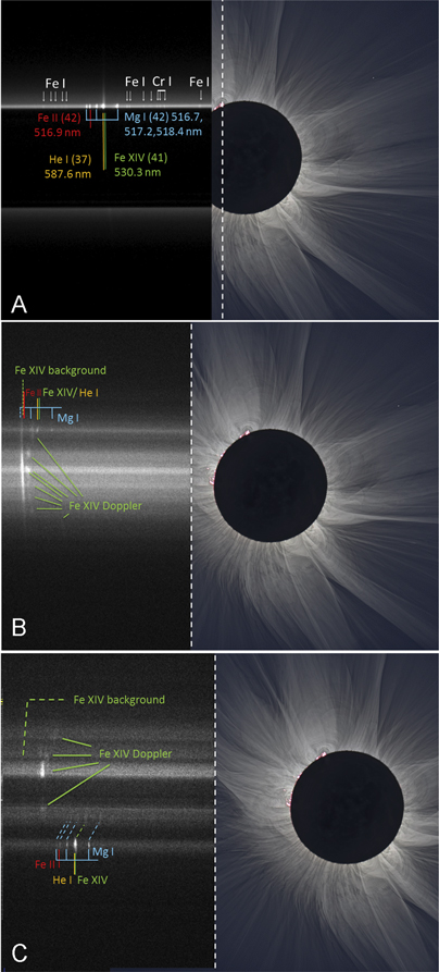
Figure 3. Two-dimensional spectra in the 41st order for Fe xiv 530.3 nm, at three different slit positions, overlaid on the white-light eclipse image. In panel (A), the slit position 354, given by the white vertical dashed line, is slightly offset from the spectrum to reveal the prominence at the north. The dark band at the center is the part obscured by the Moon. In panel (B), the slit position 378 was at 1.4 Rs. Slit position 395 in panel (C) was at 2.3 Rs. Prominence material is identified by emission from He I, a series of Fe i lines, the Mg i and Cr i triplets, such as the one intercepted in panel (A). In (B) and (C), several Doppler-redshifted Fe xiv plasmoids appear with speeds ranging from under 100 to over 1500 km s−1, with some accompanied by Fe ii, Mg i, and He i emission. The plane of sky Fe xiv emission appears over a significant fraction of the slit length in (B). In (C), the coronal background Fe xiv has weakened considerably, while many Doppler-redshifted plasmoids appear clearly.
Download figure:
Standard image High-resolution imageDetails of multiple Doppler-shifted plasmoids detected along any slit position are shown in the two-dimensional spectrum of Figure 4, for slit position 378 (the same as in Figure 3(B)), in the 41st (left) and 42nd (right) order for Fe xiv. Overlaid in the middle are five line spectra corresponding to the details of the spectra identified by the rectangular windows. B refers to the background Fe xiv emission. The other peaks refer to the Doppler-shifted ones. Emission from the Doppler-shifted Fe xiv (labeled Fe) appears in all plasmoids, and is labeled  when associated with cool inclusions. This is evident from Mg i, He i, and Fe ii emission, which appear in the top two panels. Note that these have higher speeds than the plasmoid without cool material. (The line width pointing to
  is thicker than for Mg i to show that it was a stronger emission.) The designation Fe (2) in the third and fourth panels refers to an unresolved pair of Doppler-shifted parcels. In the lower panel, where the signal is much weaker, a double-peaked Doppler-shifted Fe xiv emission, compared to the top two spectra, is clearly visible. The blue spectrum superimposed on the top spectrum is from slit position 354 (see Figure 2) when it intercepted the prominence at the limb. It is used here for comparison and as a reference.

Figure 4. Example of a two-dimensional spectrum for slit position 378 at 1.4 Rs (given in Figure 3(B)), in the 41st (left) and 42nd (right) order for Fe xiv, with details of multiple Doppler-shifted segments or plasmoids, with different speeds, along the slit. Overlaid in the middle are five line spectra corresponding to the details of the spectra identified by the rectangular windows. B refers to the background Fe xiv emission. The other peaks refer to the Doppler-shifted ones. Emission from the Doppler-shifted Fe xiv (labeled Fe) appears in all. It is labeled  when associated with cool inclusions, such as is evident from Mg i (labeled Mg), Fe ii, and He i (labeled He) emission, which appear in the top two panels and have higher speeds than the plasmoid without cool material. (The line weight for
  is thicker than for Mg i to show that it was a stronger emission.) The designation Fe (2) in the third and fourth panels refers to an unresolved pair of parcels with slightly different Doppler shifts. In panel 5, where the signal is much weaker, the Doppler shift of the Fe xiv emission is approximately twice as large as in panels 1 to 4. The blue spectrum superimposed on the top spectrum is from slit position 354 (see Figure 2) when it intercepted the prominence at the limb. It is used here for comparison and as a reference. The wavelength scale is nonlinear; the dispersion for Fe xiv is given in the lower part of the figure, with 38.6 pixels nm−1 for Fe xiv in the 41st order and 43.3 pixels nm−1 in the 42nd order.
Download figure:
Standard image High-resolution image
The 51 spectra thus acquired throughout the 2.5 minutes of totality (and a couple past totality where the coronal emission could still be detected), were comparable in complexity to the example shown in Figure 4. They yielded approximately 200 Fe xiv Doppler-shifted plasmoids, with speeds ranging from under 100 to over  km s−1, across the 2.5 × 1.5
  areal coverage spanned by the slit during that time period. Approximately 10% of them enshrouded chromospheric material, moving in tandem, and having the same spatial extent. Very few examples of faint Doppler-blueshifted lines were also found in these spectra.
5. Data Interpretation
There are several quantitative inferences that can be made from these spectra. We will focus here on the most reliable ones: the Doppler shifts and Doppler broadening.
5.1. Doppler Shifts
The Doppler shift measurements indicate that different plasmoids exhibit a wide range of velocities. In fact, a single spectrum can easily contain more than 10 plasmoids with different speeds, as shown in detail in the examples of Figures 3 and 4, with some plasmoids encapsulating chromospheric emission. The mapping of all the Doppler-redshifted plasmoids onto the white-light eclipse image of the corona is shown in Figure 5(A), where the red bounding lines refer to plasmoids that included cool emission lines. The range of speeds is given by the legend in the bottom right. The overall impression emerging from this map is that of a highly filamentary front of outflowing material away from the observer. In this map, some plasmoids seem scattered while some follow from one slit position to the next. The discrete spatial distribution of these Doppler-redshifted plasmoids is interpreted as the spatial spread of segments and/or threads of a complex, relatively large, and filamentary CME front traveling from the backside of the Sun away from the observer. Several of these filaments enshrouded cool prominence material, which seems to be clustered in two distinct locations in the corona: a slower cluster in the northeast, and a much faster cluster to the south, in the polar coronal hole region.
Figure 5. (A) Mapping of the Doppler-redshifted Fe xiv emission onto the white-light image of the corona. All plasmoids are displayed as rectangles, where their heights correspond to their spatial extent along the slit. The color-coding corresponds to different speeds inferred from the measured Doppler shifts (as shown by the legend in the bottom right). Emission from the cooler, chromospheric material, such as He i, Mg i, Cr i, and Fe ii (see examples in Figure 3), which displayed the same Doppler shift as those of the co-spatial Fe xiv plasmoids, are identified by a red border. The overlapping shadings correspond to plasmoids with different speeds at overlapping positions along the line of sight. The width of the rectangles was chosen to correspond to the distance between successive slit positions. (B) The overlay in (A) combined with the contemporaneous LASCO/C2 white-light image at 10:12 UT. (Note that the eclipse image here was rotated counterclockwise by 23 5 to match solar north—vertical up—in the LASCO/C2 image.) The area obscured by the C2 occulter is indicated by the dashed white circle. The corresponding LASCO/C2 animation covering a few hours of observations around the time of the eclipse is provided. It shows CME activity off the west limb prior to totality, but nothing off the east limb, except for faint turbulent motions at the edge of the occulter, which do not seem to emerge much beyond it.
(An animation of this figure is available.)
Download figure:
Video Standard image High-resolution image
Supporting evidence for the existence of a large front moving away from the observer comes from close inspection of the overlay in Figure 5(B), where the dashed circle traces the edge of the LASCO/C2 occulter. (Note that the eclipse image in this panel was rotated counterclockwise by 23.5 degrees to match solar north in the LASCO/C2 image.) Here, the full extent of the eclipse image, together with the Doppler map of panel 5(A), shows a superb match with the LASCO/C2 image. In this overlay, there is no evidence of disruption of coronal structures, either in the eclipse image or the LASCO/C2 image, of the type characteristic of the passage of a CME, similar to what was observed off the west limb earlier in the day (see the animation of Figure 5). There were only very minor and limited "turbulent" flows at the east limb close to the equator, which did not expand much beyond the edge of the LASCO/C2 occulter. These LASCO/C2 observations thus imply that there were no plasma motions in the plane of the sky, off the east limb in the field of view of the LASCO/C2 coronagraph. Hence, the recorded Doppler motions corresponded to material moving mostly along the observer's line of sight, in the region of space behind the occulter of the coronagraph. Additional corroborating evidence for the almost strictly anti-earthward expansion of the CME front is provided by the Doppler-redshifted plasmoids with speeds below 500 km s−1, most likely belonging to the same front observed off the south limb at the edge of the eclipsed solar disk.
Further supporting evidence for this interpretation is provided by the animation associated with Figure 5(B), which shows the LASCO/C2 white-light images a few hours before, during, and after totality. There are two processing techniques applied to the LASCO/C2 images in that animation: the Multi-Scale Gaussian Normalization Technique (MGN; Morgan & Druckmüller 2014; right panels) and the Dynamic Separation Technique (DST; Morgan et al. 2012; Morgan 2015; left panels). With MGN, the processing essentially removes the radial gradient (right panel). In the dynamic separation, what emerges are only time-varying blobs or knots (left panel). Hours before totality, a large CME was observed off the west limb (best seen in the right panel), but no event was observed off the east limb. However, careful inspection of the left panel on the DST images gives the impression of an inflow on the east and an outflow on the west of several bright knots. These can be readily interpreted as a large front moving away from the observer with its axis at an angle (which cannot be determined from these observations alone) toward the west from the line of sight. This scenario is consistent with the Doppler redshifts recorded in the eclipse data. Additional supporting evidence comes from close inspection of the processed white-light eclipse image in the south polar region. In that region, relatively broad structures, clearly distinct from the rest of the rays emanating from the poles, exhibit a sudden curvature from the radial short of 2 Rs. They can be interpreted as the backside of a filamentary front moving away from the observer. This interpretation is further supported by the number of Doppler-redshifted plasmoids detected off the south limb (see Figure 5(A)). No corroborating evidence could be obtained from the twin STEREO spacecraft, as they were behind the Sun in the Earth–Sun line at the time of the eclipse, with no signal reaching Earth. We note that even if LASCO/C2 and/or STEREO had detected this CME front, they could not have identified its temperature or the presence of cool prominence material embedded within it, since both instruments lack spectroscopic capabilities.
5.2. Doppler Broadening
The measured widths of the spectral lines can be used to infer an effective temperature, Teff, for the different ions. Assuming a Boltzmann distribution, Teff is given by (see, e.g., Esser et al. 1999)
where Ti is the ion temperature and  is the broadening due to any wave or turbulent motion along the line of sight, mi is the ion mass, and k is the Boltzmann constant. The measured line widths of Fe xiv yielded an effective temperature
  , with no significant change as a function of radial distance. We also found that the line width,
  , of both the background and Doppler-shifted Fe xiv emission were comparable. We note that Ti should be larger than the peak ionization of Fe xiv, or electron temperature
  . Since the contribution from wave motions increases with radial distance (see, e.g., Esser et al. 1999), it is then likely that Ti decreases as a function of distance; hence, the ions do not experience any heating with their expansion within the CME front. In fact, Ti is expected to decrease with supersonic expansion, as is the case with this fast CME front. While this argument applies to the CME plasma, it does not necessarily account for the fact that the Doppler broadening of the background, stationary Fe xiv was comparable, unless the contribution from non-thermal motions was the same inside and outside the CME front.
While chromospheric lines are also thermally broadened, analysis of the width of the Fe ii and Mg i spectral lines could not be achieved with reliable accuracy, since the resolution of the spectrometer is 0.03–0.04 nm. From their mass and their measured line width, and taking into account the broadening of the Mg i lines in the Fraunhofer spectrum, a maximum temperature of 105 K has been derived. On the other hand, the He i line is much more intense, and exhibits a much larger Doppler broadening, because of its low mass, than atoms and ions with higher masses at the same temperature. The width of the He i line yields an average ionic temperature of  . This value can be considered to be the maximum temperature of the cool material embedded in the CME front. We note that this maximum temperature is larger than the published electron temperature of
  (namely, the peak formation temperature of C iii 97.7 nm) reported by Akmal et al. (2001), but closer to the
  value given by Landi et al. (2010), for the cool prominence cores they observed.
6. Discussion and Conclusion
The observations presented here are not the first to show that eruptive prominence material escapes within a CME front while maintaining its ionic composition. As noted earlier, Howard (2015a, 2015b) and Wood et al. (2016) were able to follow the morphological evolution of a prominence from the Sun into interplanetary space, albeit without spectroscopic information. Spectroscopic observations with UVCS provided evidence of the presence of a cool core within a CME front (e.g., Ciaravella et al. 1997, 2000; Akmal et al. 2001; Raymond 2002; Raymond & Ciaravella 2004; Landi et al. 2010; Giordano et al. 2013; Lee & Raymond 2014). Interplanetary space measurements also reported the detection of singly ionized and low charge states of a number of ions, interpreted as the remnants of prominences within the CME front (e.g., Gosling et al. 1980; Burlaga et al. 1998; Gloeckler et al. 1999; Lepri & Zurbuchen 2010). While the observed 10% fraction of CME plasmoids accompanied by cool prominence material is higher than the 4% reported in interplanetary space measurements (Lepri & Zurbuchen 2010), it is not clear from these sole eclipse observations whether this is the norm, or whether this was an exception. Nevertheless, the relatively small, yet non-negligible, fraction of prominence material, entrained within a CME front, is consistent with the fractions reported from in situ measurements (e.g., Lepri & Zurbuchen) and from the remote sensing ultraviolet coronagraphic observations by Lee & Raymond (2014). On the other hand, one has to keep in mind that studies that suggest that eruptive prominence material can get heated up pertain only to the fate of the fraction of the prominence material that finds itself falling back toward the Sun (e.g., Filippov & Koutchmy 2002; Innes et al. 2016).
There are several novel and unique aspects of the spectral measurements in the visible wavelength range acquired with PAMIS: (1) the unambiguous identification of the emission spectrum of both hot (multi-106 K) and cool (104–105 K) plasmas, (2) the inference of line of sight Doppler shifts, and (3) the very short exposure times of 1–2 s, which enabled a large areal coverage of the corona. These features are particularly important for following the fate of eruptive material as it expands away from the Sun. Earlier breakthrough spectroscopic observations of the corona had been acquired in the ultraviolet wavelength range with UVCS (Kohl et al. 1995). While resonant excitation, also referred to as "pumping," in the presence of large outflows, was a powerful diagnostic of their radial, rather than their line of sight component, it was applicable for only a few coincidental narrow wavelength ranges (see Raymond & Ciaravella 2004). In contrast, the design of PAMIS enabled the line of sight Doppler inference for both coronal (Fe xiv and Ni xiii) and chromospheric (Cr i, Fe i and Fe ii, He i, and Mg i) emission, with no instrumental limitations. From observations of the Doppler shifts, hot plasmoids with cool inclusions, traveling in tandem at speeds ranging from under 100 to over 1500 km s−1, could be directly extracted from the spectra. From the thermal broadening of the spectral lines, the effective temperatures of the highly ionized species, e.g., Fe xiv and Ni xiii, and to a lesser extent those of the highly excited He triplet states, could also be determined. It is unfortunate that UVCS was no longer operational during the 2015 eclipse. With its diagnostic potential, it would have yielded the inference of the radial component of the outflow, thus complementing the line of sight observations in the visible and a diagnostic of the ionic temperature of the cool plasmas also complementing those reported here.
In conclusion, these first-ever spectroscopic observations in the visible wavelength range, acquired in 2.5 minutes during totality, spanning an uninterrupted projected area of  , starting from the solar surface, were enabled by the novel design of the spectrometer and its operation in higher order. They have contributed to the long-standing enigma of the fate of eruptive prominence material accompanying a CME. They showed, without a doubt, that cool and dense prominence material can survive the hot coronal environment, and its expansion into interplanetary space, enshrouded by segments of hot CME envelopes. Their presence and survival place serious new constraints on CME models (e.g., Landi et al. 2010): not only do models have to account for a source of energy to heat and accelerate a CME front, but they now have to also account for the survival of its cool core and the cool shreds embedded within it. These first-ever eclipse observations would not have been possible with any existing ground- or space-based observatories because of the absence of spectroscopic capabilities in the distance range covered by the eclipse observations. They underscore the unique opportunities provided by total solar eclipse observing conditions for in-depth exploration of the physical processes underlying the chemical evolution of the coronal plasma, and its dynamics, especially in conjunction with explosive events such as prominence eruptions and CMEs.
This work was supported by NASA grant NNX13AG11G and NSF grants AGS-1144913, AGS-1358239, and AGS-1255894 to the Institute for Astronomy of the University of Hawaii. These observations would not have been possible without help from Prof. Fred Sigernes from UNIS, who offered the use of the old Auroral Station in Adventdalen, Svalbard, Norway, and enabled the modification of the windows into glass doors. The authors are thankful to Judd Johnson, Paul Toyama, and Randy Chung for technical help with the spectrograph and its use during the total solar eclipse, to Chris Scharfenorth and Hans Eichler for providing the dichroic mirrors and filters used in the spectrometer, and to the late Heinrich Helfmeier who donated the entrance optics for the spectrometer. The authors also acknowledge help from Nathalia Alzate and Huw Morgan for access to the processed images of the ancillary SOHO-LASCO/C2 white-light data on CMEs, to Miloslav Druckmüller who produced the white-light eclipse image, and Enrico Landi for valuable discussions. The authors also thank Karen Teramura for her help with the final production of Figure 5 and the anonymous referee for valuable input.