


Abstract
It is a common practice to use 3D General Circulation Models (GCM) with spatial resolution of a few hundred kilometers to simulate the climate of Earth-like exoplanets. The enhanced albedo effect of clouds is especially important for exoplanets in the habitable zones around M dwarfs that likely have fixed substellar regions and substantial cloud coverage. Here, we carry out mesoscale model simulations with 3 km spatial resolution driven by the initial and boundary conditions in a 3D GCM and find that it could significantly underestimate the spatial variability of both the incident short-wavelength radiation and the temperature at planet surface. Our findings suggest that mesoscale models with cloud-resolving capability be considered for future studies of exoplanet climate.
Export citation and abstract BibTeX RIS
1. Introduction
The habitable zone (HZ) is defined as the region around a star in which liquid water (ocean) can be maintained for geological timescales at planet surface (Kasting et al. 1993). Traditionally, the range of the HZ is computed by cloud-free 1D radiative convective adjustment models (Kasting et al. 1993; Kopparapu et al. 2013, 2014). In these models, the effect of clouds is represented by artificially increasing the surface albedo so that surface temperature under an incoming stellar energy flux of ∼1360 W m−2 (in some of the literature this value is divided by a factor of 4 to represent the global mean condition) is close to the present-day Earth at approximately 288 K. Both the energy flux and the temperature for such tuning are for modern Earth. However, there is no reason that clouds on a different planet should behave the same way as those in modern Earth's atmosphere. In addition, the common 1D radiative convective models implicitly assume a rapidly rotating planet and cannot be used in their current form for slowly rotating planets.
The shortcoming of 1D models has led to recent efforts to study the climate of exoplanets using 3D GCMs (Leconte et al. 2013; Yang et al. 2013, 2014; Wang et al. 2014, 2016; Wolf & Toon 2014, 2015; Kopparapu et al. 2016). The effect of clouds on the inner edge of the HZ (IHZ) on tidally locked rocky planets around M dwarfs is particularly interesting because their substellar regions are likely to be fixed to certain longitudes and these planets are slow rotators. General Circulation Models (GCMs; Yang et al. 2013, 2014; Kopparapu et al. 2016) suggest that optically thick clouds should saturate substellar regions and increase the planet albedo substantially. Another study (Way et al. 2016) using a different GCM also suggests that ancient Venus might have formed thick substellar clouds if it were rotating slowly. As a result, the planet surface could remain cool even under an incident stellar radiation similar to that received by modern Venus, which pushes the IHZ closer to the host star for late-K and M dwarf systems. The typical spatial resolution of these 3D GCMs is a few degrees squared (105 km2). Thus, these models must rely on sub-grid scale parameterizations of convection and cloud microphysical processes. Sub-grid scale parameterizations remain a significant uncertainty among climate models of the modern Earth, and perhaps are even less certain for applications to exoplanetary atmospheres. A mesoscale cloud-resolving model would be preferred in order to better understand the cloud processes of exoplanets. In particular, such a model can help shed light on the robustness of the thick substellar clouds predicted for slow rotating planets around M dwarfs (Yang et al. 2013, 2014; Kopparapu et al. 2016).
In this work, we use a mesoscale cloud-resolving model (the Weather Research Forecasting model, WRF) in a 103 × 103 km2 region surrounding the substellar point on an Earth-size exoplanet using the steady state results of a 3D GCM as the initial and boundary conditions. Note that in this work we only use the cloud-resolving model over a small sub-domain of the planet due to its high-resolution and consequently large computational expenses. Comparisons between the cloud fractions, short-wavelength (SW) radiation, surface temperature, cloud water content, and precipitation patterns suggest that 3D GCMs underestimate spatial variability near the substellar point.
2. Method
We use WRF3.7.1 (Skamarock et al. 2008) with 3 km resolution, 59 vertical layers, and 5 s time steps for integration. Cloud microphysics, including ice, snow, and graupel processes in addition to liquid droplets, are calculated by the WRF Single-Moment 6-class (WSM6) scheme, which is optimized for high-resolution simulations (Hong & Lim 2006). We assume an ocean planet with zero eccentricity and a 28 day orbital period. The planetary atmosphere is assumed to contain 1 bar N2, 355 ppmv CO2, 1.7 ppmv CH4, and no ozone. The diurnal cycle of incident SW radiation in the WRF model is removed to simulate a synchronously rotating planet. A blackbody spectrum of 3700 K, with a total energy flux of 2000 W m−2, is used for the top-of-the-atmosphere stellar spectrum. RRTMG (a rapid radiative transfer model using the correlated-k method to calculate shortwave and longwave fluxes and heating rates with both efficiency and accuracy) and the Monte Carlo Independent Column Approximation method (random overlapping of sub-grid clouds) are used for both SW and longwave radiation calculations (Iacono et al. 2008).
The lateral boundary conditions and the initial conditions of the WRF model are provided by the Community Atmosphere Model version 3 (Collins et al. 2006) for an ocean planet with zero eccentricity and obliquity. CAM3 is a comprehensive Earth climate model, including 3D fluid dynamics, two-stream radiative transfer, shallow and deep convection, cloud formation and dissipation, and surface exchange processes. The model and its configuration are consistent with that used in Yang et al. (2013). The atmosphere is coupled with a 50 m slab ocean (no ocean heat transport) and thermodynamic ice is considered (ice forms at T < 271.35 K). The resolution is 2 8 and 56 in latitude and longitude, respectively. CAM3 is run for 40 years to reach an equilibrium state, and the average of the final 10 years of simulations are used to produce the WRF lateral boundary and initial conditions.
Thus, the WRF domain corresponds to ∼3 and 2 grid points in latitude and longitude (∼10 × 10 degrees) in the GCM, respectively (shown as boxes in Figures 1(A) and (C)). We also use a slab ocean and thermodynamic ice in the WRF model. The WRF model runs typically for a few months (model time) so that the large-scale patterns of all major variables (surface temperature, wind, clouds, etc.) do not vary significantly with time.
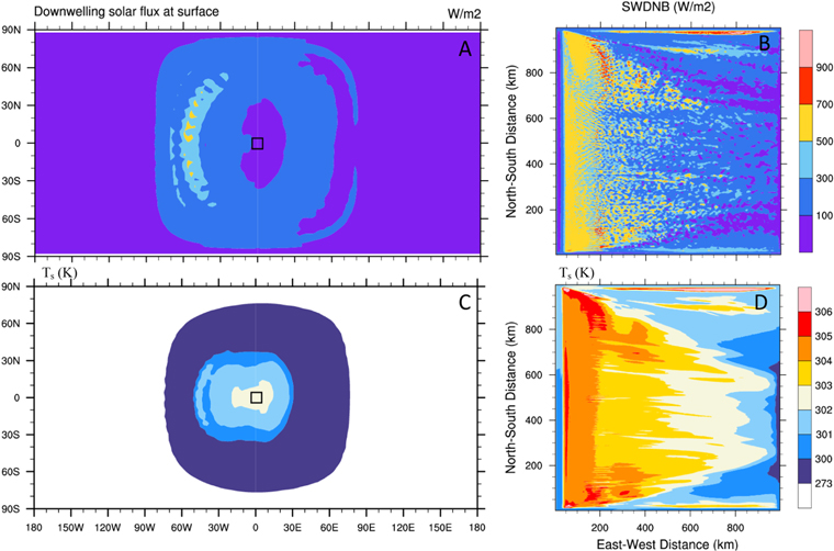
Figure 1. Downwelling short-wavelength radiation at the surface (SWDNB; upper panels) and sea surface temperature (lower panels) in the GCM (left panels) and WRF model (right panels), respectively. SWDNB in WRF shows substantial spatial variations as a result of non-uniform cloud distribution shown in Figure 2. Because of the spatial variations of SWDNB, surface temperature varies by >5 K in the WRF model. In comparison, temperature variation is <1 K because of uniform cloud distribution in the corresponding domain in the GCM. The boxes in the left panels correspond to the WRF domain.
Download figure:
Standard image High-resolution image3. Results and Discussions
Figure 1 shows the instantaneous surface downwelling SW radiation (SWDNB; upper panels) and sea surface temperature (Ts; lower panels) in the GCM (left panels) and the WRF (right panels) models, respectively. SWDNB in the GCM is ∼100 W m−2 in the region corresponding to the WRF domain as a result of uniform coverage of dense clouds (Figure 1(A)). In comparison, SWDNB in the WRF model shows variations from <100 to >900 W m−2 (Figure 1(B)). The domain-averaged SWDNB in the WRF model is ∼300 W m−2. The eastern half of the WRF domain has an averaged SWDNB of ∼200 W m−2. The overall albedo in the WRF model is ∼0.5, which is smaller than the average albedo obtained by the GCM (∼0.6) in the WRF domain. Ts in the WRF model varies by >5 K (Figure 1(D)), much greater than the <1 K variation in the corresponding domain in the GCM (Figure 1(C)). Although there are temporal variations in the exact locations of high and low SWDNB and Ts, the overall patterns of the WRF results do not change in time. In addition, WRF model runs with a 10 km resolution and a larger domain (1000 × 3000 km2) show small changes further east from the eastern boundary of the 3 km WRF runs. Thus, the WRF vertical structure has reached equilibrium.
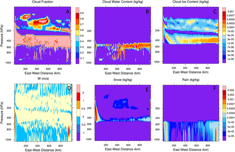
Figure 2 shows the instantaneous vertical versus east–west distributions of cloud fractions, cloud water/ice contents, vertical wind, and rain/snow along the equator of the WRF model domain. Although the cloud coverage is high between 600 and 300 hPa (Figure 2(A)), there are strong variations in the cloud water contents (Figure 2(B), ∼5–8 km altitude, liquid water phase at the base and ice phase at the top). In comparison, the cloud ice content distribution (Figure 2(C), more diffuse at lower pressure levels) is more uniform but with values almost one order of magnitude lower than those of the cloud water contents. Thus, the strong spatial variation of SWDNB in Figure 1(B) is a direct result of spatially varying water clouds in the WRF model (Figure 2(B)): dense water clouds at 500∼600 hPa levels extend from the east boundary and cover ∼50% of the WRF domain, corresponding to the region with SWDNB < 300 W m−2 (Figure 1(B)). The water content of clouds in the west half of the WRF domain is substantially lower than that in the east half of the WRF domain (Figure 2(B)). As a result, SWDNB can reach 500 ∼ 700 W m−2 in the west part of the WRF domain (Figure 1(B)).
Figure 2. Instantaneous vertical vs. east–west distributions of cloud fractions (panel A), cloud water content (B), cloud ice content (C), vertical wind (D), rain (E), and snow amounts (F) along the equator of the WRF model domain. Although the cloud coverage is high between 600 and 300 hPa (panel A), there are strong variations in the cloud water content (B). In comparison, the cloud ice content distribution (C) is more uniform but with much lower values than those of the cloud water contents. There is heavy precipitation in the form of snow at the western boundary of the simulation domain between 100 and 600 hPa level (E). The horizontal wind at these pressure levels is in the west-to-east direction in the 3D GCM, which brings water vapor from out of the WRF domain and forms snow near the western boundary of the WRF model domain. There is also snow at the eastern domain boundary between the 100 and 400 hPa levels, the likely cause of which is vertical wind (D). At pressure levels >600 hPa, the boundary effect is smaller and the rain pattern has no apparent association with the boundary (F). Overall, the distribution of clouds within the simulation domain is not influenced by the boundary conditions.
Download figure:
Standard image High-resolution image
The WRF output also shows multiple isolated weak convective cores with vertical velocities of 2–3 m s−1 and a spatial scale of ∼10 km below the liquid water cloud layer (Figure 2(D)), which are accompanied by downdrafts with larger scales. This pattern essentially rules out the presence of large-scale water clouds, which is a necessary result in the GCM considering its low spatial resolution. This is also supported by the smaller domain-averaged albedo in the WRF model than that in the GCM. While the 3 km resolution in this work can marginally resolve convective cores, ideally even higher resolution will be used to correctly represent updraft scales. There is heavy snow near the west boundary of the WRF domain between 100 and 600 hPa level, which does not reach the surface (Figure 2(E)). The GCM horizontal wind is in the west-to-east direction at a pressure >∼100 hPa (not shown), which brings water vapor into the WRF domain and forms snow. There is also snow at the eastern domain boundary between 100 and 400 hPa (Figure 2(E)), the likely cause of which is vertical wind (Figure 2(D)), which in turn is probably caused by the GCM and WRF models having different vertical mass fluxes within the domain. Although both models generally have convergence below 6 km and divergence above it, the GCM divergence extends up to 20 km, much higher than WRF's, indicating that the GCM has a deeper convective layer than WRF. As a result, the GCM easterly inflow is weaker than WRF's, which drives a vertical motion at that boundary below this divergence. We note that this adjustment circulation is confined to the boundary. At pressure levels >600 hPa the rain pattern has no apparent association with the boundaries (Figure 2(F)) and the surface rainfall of ∼1 mm/day balances the latent heat flux. The distribution of clouds within the WRF domain is not influenced by the boundary conditions.
Analysis of the vertical sounding profiles in the GCM suggests that it is close to saturation with respect to water at very cold temperatures up to 10 ∼ 100 hPa near the substellar region. In comparison, the water vapor amount in the WRF model is lower. The water–ice conversion in the GCM is described by a simple parameterization linearly associated with the difference between the freezing temperature and a threshold temperature. The water–ice conversion in the WRF model is more complicated. The WSM6 microphysics scheme in WRF considers heterogeneous and homogeneous freezing of cloud water, as well as physical processes such as initiation of cloud ice crystal and sublimation of ice (Hong & Lim 2006). We also carried out a sensitivity test using WRF Double-Moment 6 scheme (WDM6; Lim & Hong 2010), which conserves both number density and mass density in condensation calculations. In comparison, the WSM6 scheme uses prognostic cloud condensation nuclei in condensation calculations. Simulations using the WDM6 scheme in WRF show similar results. More comprehensive treatments of water and ice cloud physics could be one reason for the WRF model to have more realistic cloud behavior than that in the GCM. Although both weak, the WRF sounding profile indicates a slightly stronger convective instability (red dashed curves) in the lowest 5–6 km in comparison to that in the GCM.
4. Conclusion
Our calculations do not explore scenarios with incident SW radiation other than 2000 W m−2, which will be necessary in order to predict the IHZ of M dwarfs. In addition, the imposed boundary conditions in this work limit the implication of a regional mesoscale model to the IHZ problem. Nevertheless, our results suggest that small-scale updrafts lead to the formation of non-uniform water clouds, which results in non-uniform distribution of SW radiation at the surface and variable surface temperature in the region near the substellar point on tidally locked exoplanets around M dwarfs. Thus, more realistic treatments of convection and clouds (high spatial resolution, cloud-resolving model) in a global mesoscale model could be necessary to obtain a full picture of cloud feedbacks and climate of exoplanets around M dwarfs.
X.Z. and F.T. are supported by the Tsinghua University Initiative Science Research Program (523001028), NSFC grants 11661161014 and 41641043. This work is completed on the "Explorer 100" cluster system of Tsinghua National Laboratory for Information Science and Technology and Yellowstone supercomputer of NCAR. We thank the reviewer for helpful comments improving the quality of this Letter.