


ABSTRACT
Most previous studies on how obliquity affects planetary habitability focused on planets around Sun-like stars. Their conclusions may not be applicable to habitable planets around M dwarfs due to the tidal-locking feature and associated insolation pattern of these planets. Here we use a comprehensive three-dimensional atmospheric general circulation model to investigate this issue. We find that the climates of planets with higher obliquities are generally warmer, consistent with previous studies. The mechanism of warming is, however, completely different. Significant reduction of low clouds, instead of sea-ice cover, within the substeller region (which moves if the obliquity is non-zero) is the key in warming M-dwarf planets with high obliquities. For a total insolation of 1237 W m−2, the climate warms by 21 K when the obliquity increases from 0° to 90°. Correspondingly, the runaway greenhouse inner edge of the habitable zone shifts outward from 2500 to 2100 W m−2. The moist greenhouse inner edge, based on our crude estimation, shifts less, from 2180 to 2075 W m−2. Near the outer edge, in contrast, the climates of planets with higher obliquities are colder due to their reduced ability to maintain a hotspot at the surface. Therefore, the outer edge moves inward when obliquity is increased, opposite to the finding of previous studies on planets around Sun-like stars. Our results thus indicate that the habitable zone for M dwarfs narrows if the obliquity of their planets increases.
Export citation and abstract BibTeX RIS
1. INTRODUCTION
The habitable zone is a region surrounding a star within which a planet can maintain liquid water on its surface. Planets located inward of the inner edge of the habitable zone might undergo strong water loss, and outside of the outer edge might be globally frozen. Obliquity, an important orbital parameter, has influences on the width of the habitable zone. Most previous works focused on planets around Sun-like stars and concluded that obliquity expanded the outer edge of the habitable zone (Williams & Pollard 2003; Gaidos & Williams 2004; Spiegel et al. 2009; Ferreira et al. 2014; Armstrong et al. 2014; Linsenmeier et al. 2015). For these planets, the period of spinning is generally much shorter than the period of orbiting around their parent stars (i.e., non-tidally locked), so the stellar radiation is distributed uniformly in the zonal direction when averaged over an orbiting period. In the meridional direction, the radiation decreases from the equator to the poles when the obliquity is low, while it increases when the obliquity exceeds 54°. The polar regions of high-obliquity planets are therefore warmer, having less ice and lower planetary albedo, and it is more difficult for planets to be globally frozen (Spiegel et al. 2009; Armstrong et al. 2014; Linsenmeier et al. 2015).
M-dwarf habitable exoplanets are much closer to their parent stars than Sun-like star planets are, and are subject to a strong tidal force. Such planets are more likely to be in a tidally locked state and have a special climate pattern, the so-called "eyeball" pattern (Pierrehumbert 2010). Yang et al. (2013) showed that clouds could strongly stabilize the climate near the runaway greenhouse inner edge under synchronous rotation, and the runaway greenhouse inner edge could be pushed far closer to its parent star than previously estimated (Kasting et al. 1993; Kopparapu et al. 2013). Moreover, as will be shown later, the high-latitude regions cannot receive more (annual mean) radiation than the substellar equatorial region, even when the obliquity is as high as 90° for such planets (Figure 1). Thus, the habitability of terrestrial planets around M dwarfs should have distinct characteristics from that of non-tidally locked planets and needs to be investigated separately.

Figure 1. Incident stellar flux at the top of the atmosphere averaged over one orbit-period at 0°, 30°, 60°, 90° obliquities for 1237 W m−2. Color interval is 100 W m−2.
Download figure:
Standard image High-resolution imageMost previous works on the habitability of M-dwarf exoplanets assumed planets with zero obliquity (Pierrehumbert 2010; Wordsworth et al. 2011; Yang et al. 2013; Hu & Yang 2014; Kopparapu et al. 2016). This assumption was made because some equilibrium solutions of planetary orbits showed that obliquity could be dissipated in a relatively short timescale under a strong tidal force, resulting in a zero-obliquity state. For example, the simulation of the Kepler 186 system (Bolmont et al. 2014) showed that the obliquity dissipation timescales for the planet e (0.12 au) was on the order of only 106 years and the planet f (0.39 au) 109 years. However, zero obliquity is not the only equilibrium state. Orbital precession may cause the rotation to be locked in a "Cassini state," where the planet can retain a constant non-zero obliquity. The Cassini state, formulated by Gian Domenico Cassini in 1963, originally describes the motion of the Moon. Although the Moon is strongly tidally locked by the Earth, it still maintains an obliquity of about 6.7° (Peale 1969). It is entirely possible that habitable terrestrial planets around M dwarfs may maintain any obliquity between 0° ∼ 90° based on Cassini's law in high mutual inclinations (Dobrovolskis 2009).
In this work, we use a comprehensive three-dimensional (3D) atmospheric general circulation model to investigate how obliquity affects the habitability of planets around M dwarfs. The description of the model and the design of experiments are provided in Section 2. Results and discussion will be presented in Section 3 and our conclusion given in Section 4.
2. MODEL DESCRIPTION
The community atmosphere model version 3 (CAM3), developed by the National Center for Atmosphere Research (NCAR), is a comprehensive Earth climate model, including 3D fluid dynamics, two-stream radiative transfer, shallow and deep convection, cloud formation and dissipation, and surface exchange processes (Collins et al. 2004). This model has been extensively used in studying planetary climates and paleoclimates (Hu & Yang 2014; Wang et al. 2014). We coupled the atmosphere component with a 50 m slab ocean, which includes only thermodynamic ocean processes. The average depth of the ocean mixed layer on Earth is 50 m. We do not include ocean heat transport in the simulation. The ocean albedo is dependent on the stellar zenith angle for direct stellar radiation (ranging from about 0.025–0.39), but fixed to a constant value of 0.06 for diffuse radiation. Sea ice forms thermodynamically whenever the sea surface temperature is lower than 271.35 K.
The planetary parameters are chosen to be the same as those of the potentially habitable exoplanet GJ 667Cc (Anglada-Escudé et al. 2012; Delfosse et al. 2013). Its mass is 4.27 times of the Earth, the corresponding surface gravity is 16.2 m s−2. The eccentricity is assumed to be zero and the orbital period is 28 days. The stellar spectrum at the top of the atmosphere is generated from a 3700 K Planck function, which peaks at 0.78 μm. The geographic distribution of incident insolation is calculated according to Dobrovolskis (2009). The distance between the planet and its parent star is varied through changing the total insolation. Lacking knowledge on continent configuration, the planet is assumed to be an aqua planet. The planetary atmosphere contains 1 bar background gas (e.g., N2). The CO2 and CH4 levels are fixed at 355 ppmv and 1.7 ppmv, respectively, in all simulations. There is no ozone in the atmosphere. Four obliquities, 0°, 30°, 60°, and 90°, are tried for each insolation or star–planet distance. We will first discuss the climate at 1237 W m−2 for the four different obliquities, and then broaden the discussion to other insolation cases.
3. RESULTS
3.1. Climate at 1237 W m−2
Starting with the climate at 1237 W m−2 is a good choice for two reasons: (1) It is identical to the real insolation received by GJ 667Cc (Anglada-Escudé et al. 2012). Our discussion can be regarded as a direct study for that highly potential habitable planet. (2) It's close to the amount of solar radiation received by our own Earth, which we are quite familiar with.
The patterns of annual mean insolation (Figure 1) are consistent with previous result (Dobrovolskis 2009). The substellar point is always fixed at the center of the dayside for 0° obliquity. When the obliquity is increased to 30°, the annual mean stellar flux slightly decreases at the center of the dayside and increases in mid- to high-latitude regions. This is more so for higher obliquities so that the annual mean stellar radiation at 90° obliquity (Figure 1(d)) becomes much more uniform. However, the maximum annual mean stellar flux is still at the center of the equator. This distinct configuration has significant influence on the width of the habitable zone.
Annual mean surface temperatures and wind fields at 850 hPa are shown in Figure 2. It is not surprising that it's quite similar to Figure 1 since the surface temperature is primarily determined by the stellar radiation for this kind of terrestrial planet. The hottest regions for the four cases are all at or close to the center of the dayside. The strong heating makes the atmosphere unstable and produces large-scale upward motion. The air of the lower atmosphere converges from nearby regions, forming the specific wind pattern. Note that the wind fields are annual means, which may give the impression that the convection is always at the center of the dayside, but the actual convection closely follows the trajectory of the substellar point. The black lines are the isothermals of the freezing points (271.35 K), i.e., the sea-ice boundaries. The open water region expands significantly as obliquity increases, and can cover about half of the planet at high obliquities (Figure 2).

Figure 2. Averaged surface temperatures and 850 hPa wind fields at 0°, 30°, 60°, and 90° obliquities for 1237 W m−3. Color interval is 5 K. The black lines show the isothermals of the freezing point 271.35 K.
Download figure:
Standard image High-resolution imageThe global mean surface temperature increases with obliquity from 237 K at 0° obliquity to 258 K at 90° obliquity (Figure 3(a)). Consistent with surface temperature, global mean ice fraction decreases from 0.71 at 0° to 0.5 at 90° obliquity (Figure 3(b)), and planetary albedo decreases from 0.47 to 0.4 (Figure 3(c)). It seems that the results here agree with the previous studies on Sun-like stars: the warmer climate at a higher obliquity results from lower surface albedo due to reduced ice coverage (Spiegel et al. 2009; Armstrong et al. 2014; Linsenmeier et al. 2015). This is, however, not what happens here. The surface albedo averaged over the irradiated region (Figure 3(d)) slightly increases, rather than decreases, for non-zero obliquities, except for the case when obliquity is very close to 90°. This is not in conflict with the global ice fraction decrease because the ice fraction within the irradiated region changes very little due to its movement with the substellar point during the year.
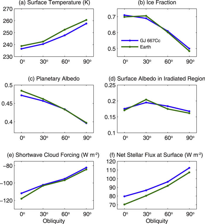
Figure 3. Climates of planets at 0°, 30°, 60°, and 90° obliquities for 1237 W m−2. (a) Global mean surface temperature, (b) global mean ice fraction, (c) planetary albedo, (d) surface albedo in irradiated region, (e) shortwave cloud forcing, (f) net stellar flux at the surface. Planetary albedo is defined as the total reflected stellar flux at the top of the atmosphere divided by the total incident stellar flux at the top of the atmosphere. Surface albedo in the irradiated region is defined as the total reflected stellar flux at the surface divided by the total downwelling stellar flux at the surface. The blue lines are for the case of GJ 667Cc surface gravity and the green lines are for the Earth surface gravity.
Download figure:
Standard image High-resolution imageThe real reason is the reduced negative cloud feedback. The shortwave cloud forcing, defined as the shortwave flux reflected by the cloud, decreases from 112 to 82 W m−2 as obliquity increases from 0° to 90° (Figure 3(e)). Correspondingly, the global mean net shortwave flux at the surface increases monotonically from 80 W m−2 at 0° obliquity to 112 W m−2 at 90° obliquity (Figure 3(f)).
The reduced negative cloud feedback is due to the movement of the substellar point. We average the quantities within a 40° circular disk centered around the substellar point in the following analysis. Changing the size of the disk does not affect the findings that will be described below as long as the disk is not too small, for which the time series of many quantities would become quite noisy. Figure 4(a) shows the meridional movement of the substellar point in one planet year. The substellar point moves past the equator at the 1st and the 15th day for non-zero obliquity, and reaches the Tropic of Cancer at the 8th day and the Tropic of Capricorn at the 22nd day. The shortwave cloud forcing is most negative when the substellar point is at the equator (1st and 15th day) and least negative when at the Tropic of Cancer (8th day) or the Tropic of Capricorn (22nd day; Figure 4(b)). The least negative shortwave cloud forcing is due to the drop of both total cloud fraction (Figure 4(e)) and total column cloud water (Figure 4(f)). The shortwave cloud forcing anti-correlates very well with the substellar surface temperatures (compare Figures 4(b) and (c)). It should be noted that the local sea surface temperature anywhere (excluding the ice-covered regions) over the globe changes very little during a 28 day period, less than 1 K; the thermal inertia of a 50 m mixed-layer ocean stabilizes the temperature.
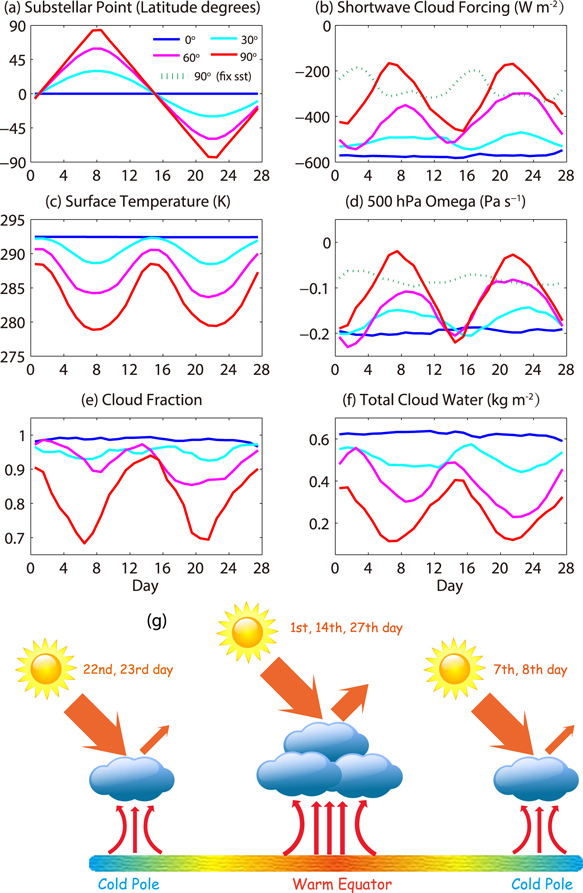
Figure 4. Variations in one planet year at four obliquities for 1237 W m−2. The orbital period is 28 days. (a) Position of the substellar point. (b) Shortwave cloud forcing averaged within 40° of the substellar point. (c) Surface temperature averaged within 40° of the substellar point. (d) Vertical velocity at 500 hPa averaged within 40° of the substellar point. (e) Cloud fraction averaged within 40° of the substellar point. (f) Total cloud water averaged within 40° of the substellar point. (g) A simplified schematic illustrating the convection and cloud cooling effect. All the quantities in this figure are daily averages. The green dashed lines in (b) and (d) are for 90° obliquity but with fixed sea surface temperature of 298 K everywhere.
Download figure:
Standard image High-resolution imageWhy do the cloud forcing and substellar surface temperature show such a high correlation? The cloud forcing is closely related to the atmospheric convection. Figure 4(d) shows the vertical velocity at 500 hPa as a measure of convective strength. Clearly, the convective strength is dramatically weaker when the star is above cold regions (days 8 and 22) than above warm regions (days 1 and 15; see also Figure 4(e)), and the cloud forcing changes correspondingly (Figure 4(b)). Such strong dependence of cloudiness on surface temperature is probably peculiar to the slow-rotating tidally locked planets (Yang et al. 2014). Due to the slow rotation, thermal-driven convective cloud is prevalent on the planet, and wave-driven cloud such as those within the mid-latitude storm track on Earth is near absent. Also due to the slow rotation, the atmosphere is in weak temperature gradient regime (Showman et al. 2013) that the horizontal temperature gradient in the free atmosphere is very small. Therefore, the convective stability of the air column is primarily determined by the surface temperature; if the surface temperature is high, it is convectively more unstable and vice versa. The higher the obliquity of the planet, the more the substellar point moves to regions with cold surface temperature (Figure 4(a)), where the convective cloud is less developed and reflectivity is therefore small. Averaged over an orbiting cycle, the planet with higher obliquity absorbs more stellar insolation than that with lower obliquity. Figure 4(g) shows a schematic illustration for what happens when the substellar point moves with latitude.
To test the above hypothesis, we carry out a simulation in which the surface temperature is fixed to be 298 K uniformly for the case of 90° obliquity (dashed green lines in Figures 4(b) and (d)). The cloud forcing and the convective strength still vary with the movement of the substellar point, but at a much subdued amplitude. This variation is owing to the non-uniform moving velocity of the substellar point; the substellar point passes the equator quickly, but stays a longer time at the Tropic of Cancer and Tropic of Capricorn where it has to reverse its direction of the moving. The largest cloud forcing is therefore obtained at these two locations where the convection is triggered (by radiative heating of the surface air) for a longer time there. This effect is largest for the case of 90° obliquity and clearly causes a shift of the phase of the shortwave cloud forcing curve (compare the position of the peaks of the red curve with other solid curves in Figure 4(b)). In any case, the result of the test indicates that the phases of the shortwave cloud forcing are controlled by the surface temperature at the substellar point.
We also tested the influence of a smaller surface gravity, 9.8 m s−2, identical to that of the Earth. The results are very similar except that the surface temperatures are 2–4 K higher (Figure 3). The higher temperature is owing to the denser/thicker atmosphere because the surface pressure is fixed in the model. We additionally tested the influence of a shallower mixed-layer depth (10 m) and a shorter synchronous rotation period (10 days), both gave very similar results, indicating that the proposed mechanism is robust.
3.2. Climate and Habitability at Other Insolations
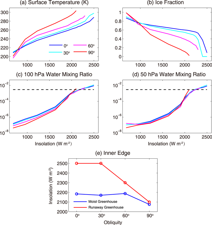
When insolation is higher than ∼1300 W m−2, the surface temperature increases/decreases almost linearly with the increase/decrease of insolation (Figure 5(a)). When insolation is reduced to below 1300 W m−2, the surface temperature still decreases linearly for low-obliquity cases, but hyper-linearly for high-obliquity cases (60° and 90°; Figure 5(a)). Therefore, although the high-obliquity planets are in general warmer than the low-obliquity planets, they freeze up more easily when insolation is reduced to very low (∼700 W m−2). If the outer edge of the habitable zone is defined as the farthest distance at which the planet can maintain liquid water on its surface (Kasting et al. 1993), the high-obliquity planets have a more inward outer edge than the low-obliquity planets. Estimating the outer edge this way has neglected the possible negative feedbacks of the carbon cycle, which may increase the atmospheric concentration of CO2 when the temperature is low (Walker et al. 1981). Dealing with the carbon cycle is out of the scope of the current study.
Figure 5. (a) Global mean surface temperatures at 0° (blue), 30° (cyan), 60° (magenta), 90° (red) obliquities for a series of insolations. (b) The same as (a) but for global mean ice fractions. (c) and (d) are the same as (a) but for 100 and 50 hPa water volume mixing ratio, respectively. (e) Moist greenhouse inner edges and runaway greenhouse inner edges.
Download figure:
Standard image High-resolution image
The results above are in contrast with previous studies on planets orbiting around Sun-like stars. They concluded that planets with higher obliquities are more resistant to the transition into a snowball state (Spiegel et al. 2009; Armstrong et al. 2014; Linsenmeier et al. 2015). The reason for the different behavior observed here is straightforward. The key for a planet to survive against being frozen up is to keep some particular region above the freezing point. This is obviously easier for the low-obliquity cases, for which the substellar point does not move around much and maintains a very high surface temperature there (e.g., Figures 1(a) and 2(a)). Sensitivity tests are done with the orbiting period being increased to 100 days. Similar trends as those in Figure 5 are observed, i.e., planets with higher obliquities enter a hard snowball more easily.
We consider two types of inner edges here: runaway greenhouse inner edge and moist greenhouse inner edge. The former refers to where positive water vapor feedback loses control and all surface water is evaporated, while the latter refers to where the efficient photolysis of water vapor and the escape of large amounts of hydrogen into space start to occur (Kasting et al. 1993). Yang et al. (2013, 2014) adopted the runaway greenhouse inner edge and used the last converged model solution as the proxy. However, it is hard to distinguish whether the model blows up due to physical instability or numerical instability. Wolf & Toon (2015) showed that the inconvergence of the model solution could be delayed when the deep convection parameterization is improved. Therefore, this method most likely underestimates the runaway greenhouse inner edge. If this method is adopted, planets with higher obliquities have much more outward inner edges than those with low obliquities (Figure 5(d)) since they are always warmer than the latter (Figure 5(a)). The runaway greenhouse inner edge is 2500 W m−2 for planets with obliquities of 0° and 30°, and decreases to 2300 W m−2 for obliquities of 60° and further decreases to 2100 W m−2 for obliquities of 90° (Figure 5(d)).
Previous estimation of the moist greenhouse inner edge used the water vapor content at the top of the climate model, i.e., 2.6 hPa (Kopparapu et al. 2016). However, certain amounts of water vapor could have already been dissociated at altitudes with greater pressure (Hu et al. 2012), in which case the escape rate of water would have been underestimated using the water vapor content at the top of the model. Accurate estimation of the moist greenhouse inner edge requires the coupling of a photochemical model and a GCM model to calculate the profiles of all hydrogen bearing species, which is beyond the scope of this work. Here we simply assume that water dissociation is efficient at the 100 hPa pressure level and water starts to be lost at a significant rate when the volume mixing ratio of water vapor at this level is higher than the critical value of 3 × 10⁻³ (Kasting et al. 1993). Both the liquid water and ice crystals in high clouds are included in the water mixing ratio estimation. Figure 5(c) shows the water mixing ratio at 100 hPa for a series of insolations. The water mixing ratio at 100 hPa is closely related to the deep convection. For planets with 0° obliquity, the star irradiates at a fixed point, maintaining intense deep convection there, even when total insolation is low. For planets with higher obliquities, the strength of deep convection decreases, but the convective area expands (Figure 4(d)). The second factor becomes more and more important as the insolation increases. In consequence, planets with high obliquities reach the critical water mixing ratio at a smaller insolation than those with low obliquities (Figure 5(c)). The results are similar if the critical escape level is assumed to be at 50 hPa (Figure 5(d)). The dependence of the moist greenhouse inner edge on obliquity is weak; it shifts from 2180 W m−2 for obliquities <60° to 2075 W m−2 for 90° obliquity (Figure 5(e)). It is consistent with the dependence estimated for the runaway greenhouse inner edge. Combined with the dependence of the outer edge on obliquity, these crude estimates indicate that the habitable zone will be narrower for planets with higher obliquities.
4. CONCLUSION
We use a comprehensive 3D atmospheric general circulation model to investigate how obliquity affects the habitability around M dwarfs. We find that the climate of planets with higher obliquities is generally warmer than those with lower obliquities. The mechanism of this warming is, however, distinctly different from that identified for planets orbiting around Sun-like stars; the warming here is due to reduced cloud reflectivity rather than surface albedo. For planets with higher obliquity, the substellar point moves to colder regions during an orbit year where convective activity is weaker and clouds are less, resulting in more stellar flux being received at the surface. Due to this warming effect, the inner edge of the habitable zone is farther from the parent star for planets with high obliquities than those with low obliquities. Based on our crude estimate, this shifting of the inner edge is significant for the runaway greenhouse edge, from 2500 W m−2 for 0° obliquity to 2100 W  for 90° obliquity, modest for the moist greenhouse edge, from 2180 W
  for obliquities lower than 60° to about 2075 W m−2 for 90° obliquity.
As to the outer edge of the habitable zone, it is found that planets with high obliquities are easier to be frozen up than those with low obliquities, therefore having an outer edge that is closer to the parent star. The traveling of the substellar point around the globe in the high-obliquity case cannot maintain a hotspot on the surface, reducing its ability to resist the tendency of entering a completely ice-covered state than in the low-obliquity case. Therefore, the influence of obliquity on the habitable zone is that the habitable zone becomes narrower when the obliquity is increased.
Y.W. and Y.H. are supported by the National Natural Science Foundation of China under grants 41375072 and 41530423. Y.L. is supported by the Startup Fund of the Ministry of Education of China. F.T. is supported by the National Natural Science Foundation of China (41175039) and the Startup Fund of the Ministry of Education of China. All of the experiments were performed on the supercomputer at the LaCOAS of Peking University.