


Abstract
Zechmeister et al. surveyed 38 nearby M dwarfs from 2000 to 2007 March with VLT2 and the Ultraviolet and Visual Echelle Spectrograph (UVES) spectrometer. These data have recently been reanalyzed, yielding a significant improvement in the Doppler velocity precision. Spurred by this, we have combined the UVES data with velocity sets from High Accuracy Radial velocity Planet Searcher, Magellan/Planet Finder Spectrograph, and Keck/High Resolution Echelle Spectrometer. Sixteen planet candidates have been uncovered orbiting nine M dwarfs. Five of them are new planets corresponding to radial velocity signals, which are not sensitive to the choice of noise models and are identified in multiple data sets over various time spans. Eight candidate planets require additional observation to be confirmed. We also confirm three previously reported planets. Among the new planets, GJ 180 d and GJ 229A c are super-Earths located in the conservative habitable zones of their host stars. We investigate their dynamical stability using the Monte Carlo approach and find both planetary orbits are robust to the gravitational perturbations of the companion planets. Due to their proximity to the Sun, the angular separation between the host stars and the potentially habitable planets in these two systems is 25 and 59 mas, respectively. They are thus good candidates for future direct imaging by James Webb Space Telescope and E-ELT. In addition, we find GJ 433 c, a cold super-Neptune belonging to an unexplored population of Neptune-like planets. With a separation of 0 5 from its host star, GJ 433 c is probably the first realistic candidate for the direct imaging of cold Neptunes. A comprehensive survey of these planets is important for the studies of planet formation.
Export citation and abstract BibTeX RIS
1. Introduction
The precision Doppler velocity revolution began in the early 1980s (Campbell & Walker 1979; Campbell et al. 1988) but proceeded slowly through the mid 1990s. Prior to the 1980s, Doppler velocity precision had been stalled at 300 m s−1 for many decades, spanning the photographic, early digital, and CCD eras. By achieving a long- term precision of 13 m s−1, the Campbell–Walker team improved Doppler precision by nearly two orders of magnitude. They also demonstrated that some Sun-like stars were intrinsically stable enough to potentially pursue measurements at higher precision.
In the era before exoplanets, Jupiter was the benchmark. Jupiter gravitationally induces a 12 m s−1 velocity variation on the Sun. A convincing 3σ-to-4σ detection of a Jupiter analog requires precision of 3 m s−1. Over the past 30 yr, two techniques have generated most of the improvement in Doppler velocity measurement precision. The first exoplanet was found by the stabilized spectrometer method (Mayor & Queloz 1995). The next 14 planets were found by the iodine absorption cell technique (Butler et al. 2006, Table 3). The iodine technique first achieved a precision of 3 m s−1 in 1995 (Butler et al. 1996), and the stabilized spectrometer first achieved a precision of 1 m s−1 in 2004 (Rupprecht et al. 2004; Pepe et al. 2011). The data sets reported in this paper come from both techniques.
Due to their lower mass, M dwarfs are the primary class of stars for which terrestrial-mass planets can be found via the precision Doppler technique. The first planet in the terrestrial-mass regime was found around the M dwarf GJ 876 (Rivera et al. 2005). Over the past decade, M dwarfs have been the principal targets for potentially habitable planets (Vogt et al. 2010; Anglada-Escudé et al. 2016; Astudillo-Defru et al. 2017; Feng et al. 2017b) because their habitable zones (HZs) are much closer to the star, and thus the potentially habitable planets have much shorter periods (and in turn produce larger semiamplitudes) than those orbiting around G stars.
The Ultraviolet and Visual Echelle Spectrograph (UVES) M Dwarf Planet survey included 33 stable nearby M dwarfs (Zechmeister et al. 2009, hereafter ZKE2009). Butler et al. (2019, hereafter B19) have reanalyzed this data set, starting with the raw images from the ESO archive.8 The updated UVES M dwarf data have previously contributed to the discovery of the terrestrial-mass planets around Proxima Cen (Anglada-Escudé et al. 2016) and Barnard's Star (Ribas et al. 2018).
Velocity data sets from UVES, the High Accuracy Radial velocity Planet Searcher (HARPS), the Carnegie Planet Finder Spectrograph (PFS) mounted on Magellan, and the High Resolution Echelle Spectrometer (HIRES) mounted on Keck have been combined to search for periodicities and confirm signals found in the newly reanalyzed UVES data. Sixteen planet candidates have been found orbiting nine nearby M dwarfs. Of these, three have previously been announced (Nakajima et al. 1995; Tuomi et al. 2014), five are newly announced low-mass planets, and eight remain candidates requiring more observations. Three additional stars with previously announced planets are also discussed.
This paper is the second of a series aiming at finding Earth analogs, and the methodology in this paper is similar to that in Feng et al. (2019, hereafter Paper I). Section 2 will describe the stars and the velocity data sets. Section 4 will examine the data sets for periodicities and embedded planetary signals. Conclusions will be presented in Section 5.
2. Radial Velocity Observations
The physical and observational properties for the stars in this study are listed in Table 1. These stars are drawn from the recently reanalyzed data from the UVES M Dwarf Planet Search (ZKE2009; B19). The first two columns of the table list common catalog designations for the stars. The spectral type, stellar mass, and V magnitudes are shown in the third, fourth, and fifth columns, respectively. These are from Table 2 of ZKE2009 and also Table 1 of B19.
Table 1. Stellar Parameters and Radial Velocity (RV) Data Sets for Stars
| Star Name | Other Name | Spectral Type | V (mag) | Stellar Mass ( ) ) |
U | K | H1 | H2 | P1 | P2 |
|---|---|---|---|---|---|---|---|---|---|---|
| GJ 27.1 | HIP 3143 | M0.5 | 11.42 | 0.53 | 62 | 8 | 50 | 0 | 0 | 0 |
| GJ 160.2 | HIP 19165 | M0V | 9.69 | 0.69 | 101 | 45 | 44 | 0 | 15 | 3 |
| GJ 173 | HIP 21556 | M1.5 | 10.35 | 0.48 | 12 | 34 | 16 | 0 | 0 | 0 |
| GJ 180 | HIP 22762 | M2V | 12.50 | 0.43 | 57 | 64 | 78 | 9 | 49 | 0 |
| GJ 229A | HD 42581 | M1/M2V | 8.14 | 0.58 | 74 | 47 | 124 | 76 | 0 | 0 |
| GJ 422 | HIP 55042 | M3.5 | 11.66 | 0.35 | 24 | 0 | 45 | 7 | 0 | 0 |
| GJ 433 | HIP 56528 | M1.5 | 9.79 | 0.48 | 167 | 33 | 86 | 0 | 39 | 4 |
| GJ 620 | HIP 80268 | M0 | 10.25 | 0.61 | 5 | 0 | 23 | 0 | 0 | 0 |
| GJ 682 | HIP 86214 | M3.5V | 10.96 | 0.27 | 49 | 0 | 20 | 0 | 0 | 0 |
| GJ 739 | HIP 93206 | M2 | 11.14 | 0.45 | 48 | 0 | 19 | 0 | 0 | 0 |
| GJ 911 | HIP 117886 | M0V | 10.88 | 0.63 | 26 | 24 | 3 | 0 | 0 | 0 |
| GJ 3082 | HIP 5812 | M0 | 11.10 | 0.47 | 10 | 0 | 42 | 0 | 0 | 0 |
Note. The values of stellar types and masses are from ZKE2009. The number of RV points are shown for the UVES (U), Keck (K), HARPSpre (H1), HARPSpost (H2), PFSpre (P1), and PFSpost (P2) data sets.
Download table as: ASCIITypeset image
Columns 6 through 11 list the number of observations taken with each spectrometer. HARPS and PFS have each had one major upgrade. In 2015 May, the fiber that feeds HARPS was replaced. In 2018 January, the old PFS CCD (4K × 4K, 15 μm pixels) was replaced with a next-generation CCD (10K × 10K, 9 μm pixels). Simultaneously, the PFS default slit width for iodine observations was reduced from 05 to 03, increasing the resolving power of the instrument from ∼80 K to ∼130 K.
All of the stars in Table 1 were observed with UVES on the VLT-UT2 telescope between 2000 and 2007 March (ZKE2009). We introduce UVES as well as other RV data used in this work as follows.
- 1.UVES. UVES is a dual arm cross-dispersed echelle spectrometer (Dekker et al. 2000). Though perhaps not fully appreciated at the time, UVES was the first "modern" precision velocity instrument. The most important criterion for a precision velocity spectrometer is resolution. With a resolution of 130 K, UVES operates at twice the resolution of earlier echelles. The calibration for precision velocity measurements is provided by an iodine absorption cell (Marcy & Butler 1992).The UVES M dwarf group used the "AUSTRAL" iodine code to model the observed spectra and produce Doppler velocity measurements (Endl et al. 2000). The AUSTRAL code is based on the modeling process outlined in Butler et al. (1996). The resulting median velocity rms of the 33 stable stars is 5.5 m s−1.The UVES data has been re-reduced using a custom raw reduction package and an upgraded version of the code from Butler et al. (1996). The median velocity rms of the stable stars is reduced to 3.6 m s−1 (B19). The velocities reported here are the "unbinned" velocities published in B19.
- 2.HARPS. HARPS has been the premier precision velocity instrument since its inception (Rupprecht et al. 2004), routinely approaching or exceeding a precision of 1 m s−1 (Pepe et al. 2011). We have obtained all the publicly reduced HARPS spectra from the ESO archive and generated velocities with the HARPS-TERRA package (Anglada-Escudé & Butler 2012).
- 3.PFS. PFS (Crane et al. 2010) is a purpose-built iodine precision velocity echelle that is used on the 6.5 m Magellan II (Clay) telescope. Like HARPS, it is designed to maximize thermal and mechanical stability. With the exception of the focus, PFS has no moving parts. It is mounted on an optical bench in a thermal insulating enclosure. The interior of the enclosure is heated to 27 °C, and the temperature is maintained to ±0.01 °C. The focus of PFS does not change with time. We have reduced the PFS data with our custom raw and velocity reduction packages.
- 4.Keck. The Keck HIRES program is the longest continuously running precision velocity survey, having commenced in 1996. HIRES (Vogt et al. 1994) is permanently mounted on the Nasmyth platform on the Keck I 10 m telescope. An iodine cell is used for the wavelength calibration. Most of the first 200 extrasolar planets were found with this system (Butler et al. 2006). With a 086 slit, the resolution of HIRES is 60 K. As a result, the long-term precision of HIRES is 2–3 m s−1. The data for this program are from the analysis of Butler et al. (2017). We have reduced all the data, starting with the raw images, with our custom raw and velocity reduction packages.
Nine of the stars listed in Table 1 are found to host new planets. The remaining three stars have previously announced planets (Tuomi et al. 2014, hereafter T14). We are able to confirm some of the planets from T14, but not all of them. We discuss this discrepancy in Section 4.3. Figure 1 shows the full Doppler velocity data sets for the 12 stars. There is significant temporal overlap between the data sets for many of the stars.

Figure 1. Doppler velocity data sets of UVES, Keck, HARPS, and PFS for the 12 stars reported in this paper. The RV sets are shifted to zero mean for optimal visualization.(The data used to create this figure are available.)
Download figure:
Standard image High-resolution image3. Method
The method used in RV data analysis in this work is similar to that used in Paper I. We briefly introduce it in this section.
3.1. RV Model and Model Selection
The RV model is composed of the signal and noise components. The signal component for Np planets for the kth data set is
where Ki is the semiamplitude of the stellar RV variation caused by the perturbation of the ith planet;  is the true anomaly derived from the orbital period Pi, eccentricity ei, and the reference mean anomaly M0 by solving Kepler's equation; and
  and
and  are, respectively, the intercept and slope of a linear trend used to model instrumental bias and secular acceleration. For long-period signals with period comparable to the RV data time span, we replace the linear trend by an offset to avoid degeneracy between long-period signals and the linear trend.
The time-correlated (or red) noise in the kth RV set is modeled by the  -order moving average model (MA(q)),
where wik is the amplitude of the ith MA component for the kth RV set, and  is the timescale of the MA model for the kth RV set, and
  is the measured RV at epoch
  in the kth set. The full RV model for the kth RV set is

The logarithmic likelihood for the combination of Ns RV sets is
where sk is the white-noise jitter for the kth RV set,  is the measured RV uncertainty at epoch tj in the kth RV set, and Nk is the number of RV points in set k.
The difference in the Bayesian information criterion (BIC) of two models is

where  and
and  are, respectively, the maximum likelihoods of models 1 and 2,
  is the number of all RV points for a target, and n1 and n2 are, respectively, the efficient numbers of free parameters in models 1 and 2. Following Kass & Raftery (1995), we convert
  to a Bayes factor (BF) by assuming a single Gaussian posterior distribution,
  . This assumption is not inappropriate as long as the posterior is dominated by a single signal. Moreover, the threshold
  or
or  is appropriate for model selection according to Kass & Raftery (1995). This is also confirmed by a comparison of various information criteria and BF computation methods based on analyses of synthetic and real RV sets in Feng et al. (2016). The order q of the MA model is determined through Bayesian model comparison by selecting the model with the highest order which passes the
  criterion. Hereafter, we use
  as an abbreviation of
  .
.
3.2. Posterior Sampling and Noise Model Selection
We use adaptive Markov Chain Monte Carlo (MCMC) developed by Haario et al. (2006) to sample the posterior distribution of model parameters. We adopt a semi-Gaussian prior ( ) for eccentricity in order to capture the broad feature of eccentricity distribution found in Kepler planet samples (Kane et al. 2012; Van Eylen et al. 2019), a logarithmic uniform prior for orbital period and MA timescale, and uniform priors for other parameters. Because we have adopted an informative prior for eccentricity, we test the sensitivity of our results to eccentricity priors for strong planetary candidates in Appendix A and do not find significant dependence of parameter values on priors, although minor sensitivity might be found for weak planetary candidates.
For a given model, we sample the posterior through multiple tempered (hot) MCMC chains to identify the global maximum of the posterior. We then use nontempered (cold) chains to sample the global maximum found by hot chains. From the posterior sample, we infer the parameter at the maximum a posteriori (MAP) and use quantiles to estimate parameter uncertainties. This is explained in detail in Paper I.
To select the optimal noise model, we calculate the maximum likelihood for an MA model using the Levenberg–Marquardt optimization algorithm (Levenberg 1944; Marquardt 1963). We calculate ln(BF) for MA(q + 1) and MA(q). If ln(BF) < 5, we select MA(q). If ln(BF) ≥ 5, we select MA(q + 1) and keep increasing the order of MA model until the model with the highest order passing the ln(BF) ≥ 5 criterion is found. Readers are referred to Feng et al. (2017a) for details.
3.3. Signal Selection Criteria
Following Paper I, we select signals that are statistically significant, independent of noise models, not correlated with stellar activity, and consistent in time. Here we reiterate the main points of these criteria which are described in Paper I.
The noise models we have used to calculate BF periodograms (BFPs; Feng et al. 2017a) are the white-noise model (a constant jitter is used to fit excess noise), the first-order MA model (MA(1); Tuomi et al. 2013), and the first autoregressive model (AR(1); Tuomi & Anglada-Escudé 2013). The evidence for signal is considered to be strong if the logarithmic BF is larger than 3 (i.e.,  ) or equivalently, its BIC is larger than 6 (Kass & Raftery 1995). A signal is considered to be very strong or significant if
  . However, the exact number of free parameters k is not known. A Keplerian model for a circular orbit has three free parameters while an eccentric orbit needs five parameters to model. Hence, we define k = 3 and k = 5 as the boundaries for the real BIC value, corresponding to
  and
and  , respectively. Signals with
  are selected as planet candidates. Because the sinusoidal function is used in the calculation of BFPs, we use
  as a threshold to visualize the significance of a signal. The real significance of a signal is determined through posterior sampling combined with the BF threshold.
To exclude signals due to stellar activity, we calculate BFPs for activity indices and window functions for each data set and find whether there is an overlap between RV signals and activity signals. To assess the consistency of signals over time, we show the moving periodogram for those signals whose phase is well covered by the RV data. Specifically, the BFP is calculated for the RVs measured within a time window. The time window moves with a certain time step until the whole time span is covered. The BFPs for all time windows form a two-dimensional map of periodogram powers. Considering that the number of RVs in a time window changes when the window moves, the BFP for a given step is normalized so that the power varies from 0 to 1. For signals with orbital period comparable with the data time span, one should not rely on the moving periodogram as the single diagnostic tool. Because the RVs are typically not measured in a uniform way, the consistency of a true signal may depend on the sampling cadence even if the power is normalized (Paper I). However, it is easy to identify false positives if inconsistency is found at high-cadence epochs with a timescale comparable to or longer than the signal period.
The moving periodogram is also known as time–frequency analysis in analyses of regularly spaced time series (Cohen 1995). Compared with time–frequency analysis, the moving periodogram accounts for floating linear trend, red noise, jitter, and irregularity in RV data (Feng et al. 2017a). Thus, we follow Feng et al. (2017a) by using a "moving periodogram" to distinguish between these two types of analyses. Similar techniques have been developed by Mortier et al. (2015), Mortier & Collier Cameron (2017) to test the sensitivity of signals to sample size.
4. Results
4.1. Planetary Signals
We select those signals which have  , do not display significant activity, and are independent of the chosen noise model. We show the orbital solutions for these signals in Table 2. Notes are attached for signals to show whether they are temperate and to show concerns about their quality. Planet candidates with notes of "OV," "L3," and "NC" are to be further confirmed while candidates with "HZ" or without any notes are likely to be real planets. Based on these considerations, we find eight planet candidates including two reported by T14, which need to be confirmed. They are GJ 173 b, GJ 229A b, GJ 433 c, GJ 620 b, GJ 620 c, GJ 739 b, GJ 739 c, and GJ 911 b.
Table 2. Parameters for Planet Candidates
| Planet |
 ( ( ) ) |
a (au) | P (days) | K (m s−1) | e | ω (deg) | M0 (deg) | Note |
|---|---|---|---|---|---|---|---|---|
| GJ 173 b | 9.5 ± 2.1 | 0.200 ± 0.007 | 47.304 ± 0.254 | 2.78 ± 0.59 | 0.10 ± 0.06 | 231 ± 94 | 222 ± 106 | NI |

|

|

|

|

|

|

|
||
| GJ 180 b | 6.49 ± 0.68 | 0.092 ± 0.003 | 17.133 ± 0.003 | 3.25 ± 0.26 | 0.07 ± 0.04 | 276 ± 26 | 314 ± 25 | T14 |

|

|

|

|

|

|

|
||
| GJ 180 d | 7.56 ± 1.07 | 0.309 ± 0.010 | 106.300 ± 0.129 | 2.08 ± 0.26 | 0.14 ± 0.04 | 155 ± 127 | 235 ± 85 | HZ |

|

|

|

|

|

|

|
||
| GJ 229A c | 7.268 ± 1.256 | 0.339 ± 0.011 | 121.995 ± 0.161 | 1.93 ± 0.30 | 0.19 ± 0.08 | 121 ± 33 | 154 ± 36 | HZ |

|

|

|

|

|

|

|
||
| GJ 229A b | 8.478 ± 2.033 | 0.898 ± 0.031 | 526.115 ± 4.300 | 1.37 ± 0.31 | 0.10 ± 0.06 | 199 ± 71 | 212 ± 82 | OV, T14 |

|

|

|

|

|

|

|
||
| GJ 229B | 426.389 ± 57.505 | 17.585 ± 2.477 | 45925.334 ± 9473.054 | 15.48 ± 1.47 | 0.07 ± 0.05 | 199 ± 93 | 206 ± 114 | N95 |

|

|
|

|

|

|

|
||
| GJ 422 b | 11.07 ± 1.12 | 0.111 ± 0.004 | 20.129 ± 0.005 | 4.47 ± 0.34 | 0.11 ± 0.04 | 265 ± 18 | 224 ± 160 | |

|

|

|

|

|

|

|
||
| GJ 433 b | 6.043 ± 0.597 | 0.062 ± 0.002 | 7.3705 ± 0.0005 | 2.86 ± 0.21 | 0.04 ± 0.03 | 154 ± 106 | 170 ± 114 | T14 |

|

|

|

|

|

|

|
||
| GJ 433 d | 5.223 ± 0.921 | 0.178 ± 0.006 | 36.059 ± 0.016 | 1.46 ± 0.24 | 0.07 ± 0.05 | 159 ± 82 | 219 ± 102 | |

|

|

|

|

|

|

|
||
| GJ 433 c | 32.422 ± 6.329 | 4.819 ± 0.417 | 5094.105 ± 608.617 | 1.75 ± 0.31 | 0.12 ± 0.07 | 242 ± 55 | 213 ± 51 | L3, T14 |

|

|

|

|

|

|

|
||
| GJ 620 b | 7.26 ± 1.16 | 0.063 ± 0.002 | 7.655 ± 0.004 | 3.41 ± 0.49 | 0.08 ± 0.05 | 182 ± 110 | 180 ± 107 | NC |

|

|

|

|

|

|

|
||
| GJ 620 c | 6.97 ± 2.34 | 0.147 ± 0.005 | 27.040 ± 0.429 | 2.15 ± 0.70 | 0.09 ± 0.06 | 154 ± 110 | 204 ± 108 | NC, L3 |

|

|

|

|

|

|

|
||
| GJ 739 b | 9.75 ± 1.86 | 0.211 ± 0.007 | 45.357 ± 0.043 | 2.45 ± 0.44 | 0.08 ± 0.06 | 169 ± 104 | 178 ± 99 | NC |

|

|

|

|

|

|

|
||
| GJ 739 c | 42.63 ± 6.23 | 0.687 ± 0.023 | 266.985 ± 0.745 | 5.91 ± 0.77 | 0.07 ± 0.04 | 197 ± 88 | 150 ± 113 | NC |

|

|

|

|

|

|

|
||
| GJ 911 b | 6.9 ± 1.3 | 0.033 ± 0.001 | 2.7889 ± 0.0004 | 4.31 ± 0.73 | 0.08 ± 0.06 | 181 ± 108 | 184 ± 103 | NC |

|

|

|

|

|

|

|
||
| GJ 3082 b | 8.2 ± 1.7 | 0.079 ± 0.003 | 11.949 ± 0.022 | 3.94 ± 0.74 | 0.22 ± 0.11 | 121 ± 54 | 150 ± 56 | |

|

|

|

|

|

|

|
||
Note. The minimum mass, semimajor axis, period, RV semiamplitude, eccentricity, and mean anomaly at the reference epoch are denoted by  , a, P, K, e, ω, and M0, respectively. The mean and standard deviation of each parameter are estimated from the posterior samples drawn by MCMC. For each parameter, the value at the MAP and the uncertainty interval defined by the 1% and 99% quantiles of the posterior distribution are shown below the values of the mean and standard deviation. The note for a planet candidate shows that it is in the HZ defined by Kopparapu et al. (2014), or it is reported in T14 or in Nakajima et al. (1995, hereafter N95), or it partly overlaps with activity signals ("OV"), or
  is less than 3 ("L3"), or it is not found in individual data sets (NI). If a signal is not consistently significant over time, due to a lack of enough data, we add the note "NC" to show our concern. For the planet candidates reported by T14, we keep their original names and assign new names to new planet candidates identified in this work. We use boldfaced planet names to indicate a reliable detection of planet, use italics to indicate planet candidates needing to be confirmed by more observations, and use normal font to indicate confirmation of previously reported signals.
Download table as: ASCIITypeset image
Our analyses support a Keplerian origin for GJ 180 b and GJ 433 b detected by T14 as well as GJ 229B discovered by Nakajima et al. (1995). We identify five new planets corresponding to RV signals which are statistically significant, unique, and consistent over time, and robust to the choice of noise models. They are GJ 180 d, GJ 229A c, GJ 422 b, GJ 433 d, and GJ 3082 b. Two of the five new planets have masses in line with super-Earth-type planets located in the HZs of their hosts.
We show the phase curve and residuals for all planet candidates in Figure 2. Because the residuals probably contain insignificant planetary and activity signals, the traditional test of goodness of fit may not be suitable for this type of residual. Nevertheless, we report the results of various tests in Table 4 and discuss their implications for the case of irregularly and sparsely sampled RV time series.
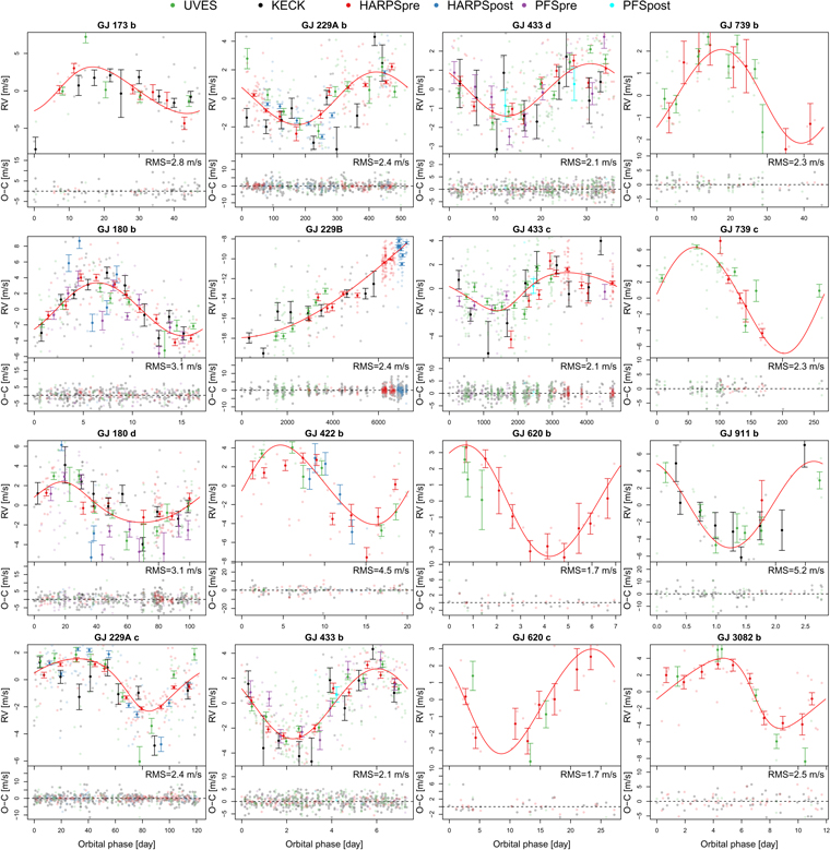
Figure 2. Phase curves and corresponding residuals for all planet candidates are shown. The instruments are encoded by different colors and are shown on top of all panels. The error bars show the error-weighted average RVs in 10 evenly separated time bins. The best orbital solution is determined by the MAP values of orbital parameters. The rms of the residual RVs after subtracting all signals is shown in each panel.
Download figure:
Standard image High-resolution imageIn Figure 3, we visualize the distribution of planet mass and period for the planet candidates detected in this work and the planets collected by the NASA Exoplanet Archive9 (Akeson et al. 2013). While most planets are located in the crowded region in the parameter space, GJ 433 c is a Neptune on a year-long orbit. The detection of wide-orbit Neptunes around M dwarfs has thus far been rare. Moreover, GJ 433 c stands out as a unique detection of a wide-orbit cold super-Neptune. Previous detections of cold Neptunes have come from the microlensing technique (e.g., Sumi et al. 2010). Our confirmation of the previously suspected super-Neptune around GJ 433 (T14) demonstrates the ability of increasingly precise Doppler velocity measurements and longer Doppler baselines to probe this rarely explored population.

Figure 3. Distribution of planet mass and period for archived exoplanets, solar system planets, and the ones found in this work. The shapes and colors of markers are combined to show different planets. The two habitable-zone planets, GJ 180 d and GJ 229A c, are denoted by black borders.
Download figure:
Standard image High-resolution imageWe compare the two temperate planets, GJ 180 d and GJ 229A c, with the conservative sample of potentially habitable exoplanets collected by PHL10
in Figure 4. GJ 229A c is located within the conservative HZ defined by Kopparapu et al. (2014), while GJ 180 d is located near the HZ outer edge corresponding to the maximum greenhouse limit. GJ 180 d is in a wider orbit and thus receives less stellar radiation than GJ 229A c. However, GJ 180 d and GJ 229A c have minimum masses of 7.6 and 7.2  . Thus, they might not be rocky as the composition of super-Earths are not well understood.

Figure 4. Distribution of incoming stellar flux and stellar efficient temperature for known planets and planets detected in this work. The conservative HZ is defined by the runaway greenhouse and maximum greenhouse limit (Kopparapu et al. 2014). The optimistic HZ is defined by the recent Venus and early Mars limit. The effective temperature and luminosity of GJ 229A c and GJ 180 d are from Schweitzer et al. (2019). The parameters for exoplanets are from the NASA Exoplanet Archive. The error bars for GJ 229A c and GJ 180 d are the uncertainties of effective temperature and effective stellar flux, due to measurement errors in stellar mass and luminosity.
Download figure:
Standard image High-resolution imageWe discuss the results for each planet candidate in the following subsection. For each planet candidate, we show the BFPs for RV data sets and activity indices. We label each panel with "Pn," where n is a number to identify the panel. We also calculate the moving periodogram to show the time consistency of signals. The components in the BFP figures are described in detail in the caption of Figure 5. The components in the moving periodogram figures are introduced in Figure 6.
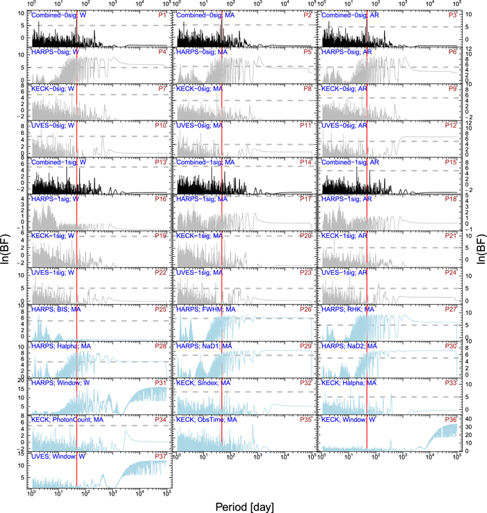
Figure 5. BFPs for GJ 173. The black BFPs are calculated for the combined data subtracted by signals subsequently while the gray BFPs are for individual data sets. The light-blue BFPs are for activity indices and window functions. The top-left legend in each panel denotes the name of RV data set or activity index and the number of signals subtracted from the data. The top-right legend in each panel shows the panel number for reference. The red lines denote the planetary signal at a period of 47.3 days. The horizontal dashed lines show the threshold of ln(BF) = 5.
Download figure:
Standard image High-resolution image
Figure 6. Moving periodogram for GJ 173. The top two panels show the same combined RV data subtracted by the best-fit MA red noise. The bottom-left panel shows the BFPs as a function of period and time window with a size of about 2000 days (double the width of the gap between the left y-axis and the left edge of the color-coded BFPs). The bottom-right panel is a zoom-in of the bottom-left panel to optimize the visualization of the signal. The annual aliases of the 47.3 day signal at periods of 54 and 42 days are visible and coded in red.
Download figure:
Standard image High-resolution image4.2. Individual Candidates
- 1.GJ 173 (HIP 21556). GJ 173 b has a minimum mass of 10.7
 and an orbital period of 47.3 days. It is identified in the combined UVES, Keck, and HARPS data (see Figure 5). The activity indicators do not have significant power at this period. In Figure 6, the moving periodogram shows consistent significance at the period of 47.3 days. However, this signal cannot be identified in individual data sets. Hence, we add a note in Table 2 to show our concern.
 - 2.GJ 180 (HIP 22762). GJ 180 b and d have minimum masses of 6.75 and 7.49, respectively. The corresponding RV signals with periods of 17 and 106 days are identified in the combined UVES, Keck, HARPS, and PFS data. The 17 day signal reported by T14 is identified while the 24 days in T14 is not found to be significant, as shown in Figure 7. There is no significant power at periods of 17 and 106 days in the BFPs for the activity indicators. In Figures 8 and 9, we see unique and consistent significance over time for these two signals. Therefore, our analyses support a Keplerian origin of these two signals. The outer planet is a super-Earth located in the HZ. As the host star is only 12.4 pc from the Sun, the separation between the primary and the potentially habitable planet is about 25 mas.
- 3.GJ 229A (HD 42581). There are three signals with periods of 122, 520, and 49,000 days found in the combined Keck, HARPSpre, HARPSpost, and UVES data. They corresponds to minimum masses of 7.93, 10.0, and 515. GJ 229A c is probably a super-Earth with an orbital period of 122 days and is located in the temperate zone corresponding to a period interval of days (Kopparapu et al. 2014). As shown in Figure 10, it does not overlap with any activity signals. It is strong in the HARPSpre, HARPSpost, and UVES sets (e.g., P35, P39, P43, and P44). It is evident from the moving periodogram shown in Figure 11 that this signal is unique and is consistent over time, although it is most significant in recent epochs due to high-cadence sampling. Although this signal is close to one-third of one year, it is unlikely an annual alias because no strong powers around one-year and half-year periods are found in the BFPs nor in the moving periodograms.The phase curve shown in Figure 2 demonstrates a good fit to the UVES and HARPS data. This strongly supports a Keplerian origin. This temperate super-Earth system is nearby (5.75 pc), and the separation between the primary and GJ 229 c is about 59 mas, making it suitable for future direct imaging by facilities such as NIRSS on the James Webb Space Telescope (Greenhouse 2016) and EPICS on E-ELT (Marchiori et al. 2008). GJ 229A b has an orbital period of 523 days that is close to the period of 470 days reported by T14 who used the old HARPS and UVES data sets. The 471 day signal in T14 is probably related to the new 520 day signal found in our analysis. However, there are strong powers around this period in the BFPs for activity indices shown in panels P57, P58, P59, P60, P63, and P64 of Figure 10 although the peaks in the activity index BFPs are quite broad. If we consider the activity signal in P57 as typical, the long-period activity signal probably has a period between 200 and 2000 days. Thus, any long-period RV signal would be identified as an activity signal if overlaps between RV and activity signals are considered as the only diagnostic metric. Considering the limitation of this criterion and that the signal is unique and significant in the RV BFPs shown in panels P31, P32, and P33 of Figure 10, it is likely related to a planet. The moving periodogram shown in Figure 12 supports a reasonable time consistency and displays higher significance in the recent high-cadence HARPS data.The long-period signal at a period of about 50,000 days corresponds to GJ 229B, which is a brown dwarf detected through direct imaging (Nakajima et al. 1995; Golimowski et al. 1998). Thanks to a time span of nearly 20 yr of combined data, we exclude an orbital period of less than 15,800 days with a false alarm probability of 1%. The minimum mass of GJ 229B is about 515 or 1.62 , which is much lower than the estimation of ∼20 by Nakajima et al. (1995) based on cooling models of brown dwarfs and the recent estimation of 72 by Brandt et al. (2019) based on a combined analysis of KECK RVs and astrometric data. This suggests a relatively face-on orientation for the system, consistent with an inclination of deg estimated by Brandt et al. (2019). As the orbital period of GJ 229B is much longer than the RV time span, we do not show the moving periodogram for this signal. In Figure 10, we see a significant activity signal at a period of 278 days in P49, P50, P51, P52, P53, P61, P63, and P64. It is probably caused by stellar rotation or magnetic cycles.
- 4.GJ 422 (HIP 55042). A signal at a period of 20.129 days with a minimum mass of 10.4 is identified in the combined UVES, HARPSpre, and HARPSpost data. This signal is not found in activity indices (see Figure 13) and is relatively consistent over time (Figure 14). It is found to be strong in all of the three sets (P4 to P12) as well as in the combined set (P1 to P3). A signal of around eight days is found to have strong powers in the BFPs for the Hα of HARPSpre (P35) and for other indices (P31 and P37). The 26 day signal reported by T14 is not as significant as this signal, as seen in Figure 13. Considering that these two signals are probably related, we still use GJ 422 b to name this candidate.
- 5.GJ 433 (HIP 56528). There are three signals with periods of 7.37, 36.1, and 5000 days and minimum masses of 5.94, 4.94, and 28.8 found in the combined HARPS, Keck, PFSpre, PFSpost, and UVES data (see Figure 15). The 7.37 day signal is found by T14. This signal is unique and consistent over time, as shown by the moving periodogram in Figure 16. The 36 day signal is significant in the HARPS set and shows high ln(BF) in the BFPs for Keck, PFS, and UVES. The moving periodogram shown in Figure 17 demonstrates that this signal is unique and consistent over time.
T14 find a long-period signal with an optimal period of 2950 days, although the period is consistent with any values larger than 1900 days. In Figure 15, we see strong power around 2947.6 days in the BFP for the HARPS data when the 7.37 and 36 day signals (P34–36) have been subtracted. However, the signal does not appear in the BFPs for the residuals of PFSpre (P40–P42) and UVES (P43–P45). With more data sets spanning a longer period (see the phase curve for GJ 433 d in Figure 2), we are able to constrain the period to be 5093 ± 610 days. In the BFPs for the combined residuals, the power around 5000 days is high in the BFP for the white-noise model (P31) and is a bit lower in the BFPs for the MA and AR models (P32–P33). This effect for long-period signals is expected because a linear trend is fit to the data in the calculation of BFP. Thus, we rely on a full MCMC posterior sampling to identify and constrain the signal, leading to for the three-planet model compared with the two-planet model. Because the orbital period of this signal is longer than the RV time span, the moving periodogram is not able to demonstrate time consistency. This signal corresponds to a super-Neptune with a semimajor axis of about 4.7 au, equivalent to a separation of 05 to GJ 433.As Figure 15 shows, the activity signal at a period of 107.3 days is significant in the BFPs for the FWHM and NaD2 indices from HARPS. Thus, we consider this signal as the rotation period, differing from the 73.2 ± 16.0 days inferred by Suárez Mascareño et al. (2015) using the Ca ii H&K and Hα indicators.
- 6.GJ 620 (HIP 80268). Two signals with periods of 7.65 and 27.2 days and minimum masses of 7.38 and 10.08 are identified in the combined UVES and HARPS data. This signal is not found in the activity indices (see Figure 18). Considering there are only 5 UVES and 23 HARPS RV data points, we use one time window to cover the former and one window to cover the latter to calculate the moving periodogram. In Figure 19, the power around 7.65 days is consistent over time but is not unique for the UVES data, due to the poor sampling of the orbital phase. Similarly, the 27.2 day signal shows time consistency in the periodogram shown in Figure 20.
- 7.GJ 739 (HIP 93206). Two signals with periods of 45.3 and 266 days and minimum masses of 8.49 and 47.52 are identified in the combined UVES and HARPS data. These signals are not found in activity indices (see Figure 21). In Figure 22, the moving periodogram shows time consistency for these signals although the signal is not unique in the recent HARPS data, due to poor sampling. The moving periodogram shown in Figure 23 demonstrates the time consistency for the 266 day signal.
- 8.GJ 911 (HIP 117886). A signal at a period of 2.79 days and with a minimum mass of 8.21 is identified in the combined UVES, HARPS, and Keck data. As seen from Figure 24, this signal is not found in activity indices (see Figure 24). This signal is significant in the UVES set (P7 and P9), and the corresponding suggests high statistical significance, although it is not found to be significant in the BFPs for the combined data set (P1, P2, and P3). To visualize the time consistency of this signal, we create the moving periodogram by calculating the BFP for the RV points in a time window. The window moves in 10 steps to cover the whole RV time span. The BFPs are normalized such that the maximum ln(BF) difference for a time window is one. The size of the window is automatically determined such that it is large enough to allow a minimum number of 10% of the total number of RV points in each of the 10 windows (see Paper I for details). We show the moving periodogram for GJ 911 in Figure 25. Although the normalized ln(BF) around 2.79 days is high for the recent Keck measurements (>2500 days after the first epoch), there are multiple signals with similar significance. The power around 2.79 days for the previous UVES RVs is strongly evident despite having less contrast compared with other periods. Thus, the overall evidence favors a time-consistent signal at a period of 2.79 days. The other signals are either not as significant or not as consistent as this signal.
- 9.GJ 3082 (HIP 5812). A signal around 11.9 days with a minimum mass of 8.77 is identified in the combined HARPS and UVES data. In Figure 26, the BFPs for the data show high and unique power at this period (P1, P2, and P3). Compared with the white-noise BFPs, the red-noise BFPs show more unique and significant power for this signal. We also identify a significant activity signal at a period of 123 days in the BFPs for the FWHM and NaD2 of HARPS. We show the moving periodogram for this signal in Figure 27. This signal is unique and consistent over time, although multiple aliases are shown in the BFP for the recent HARPS RVs.


![$[114,315]$](https://content.cld.iop.org/journals/0067-0049/246/1/11/revision1/apjsab5e7cieqn148.gif)


Figure 7. BFP for GJ 180. The red lines denote the signal at periods of 17 and 106 days, which are subtracted from the raw RV data subsequently to calculate residual BFPs. The P80 panel shows the BFP for the TESS photometry data (Ricker et al. 2014).
Download figure:
Standard image High-resolution image
Figure 8. Moving periodogram for GJ 180 b. The annual aliases of the 17.9 day signal at periods of 16.3 and 17.9 days are also visible.
Download figure:
Standard image High-resolution image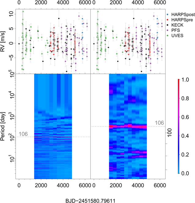
Figure 9. Moving periodogram for GJ 180 c. The annual aliases of the 106 day signal at periods of 82 and 149 days are visible though not consistent over time.
Download figure:
Standard image High-resolution image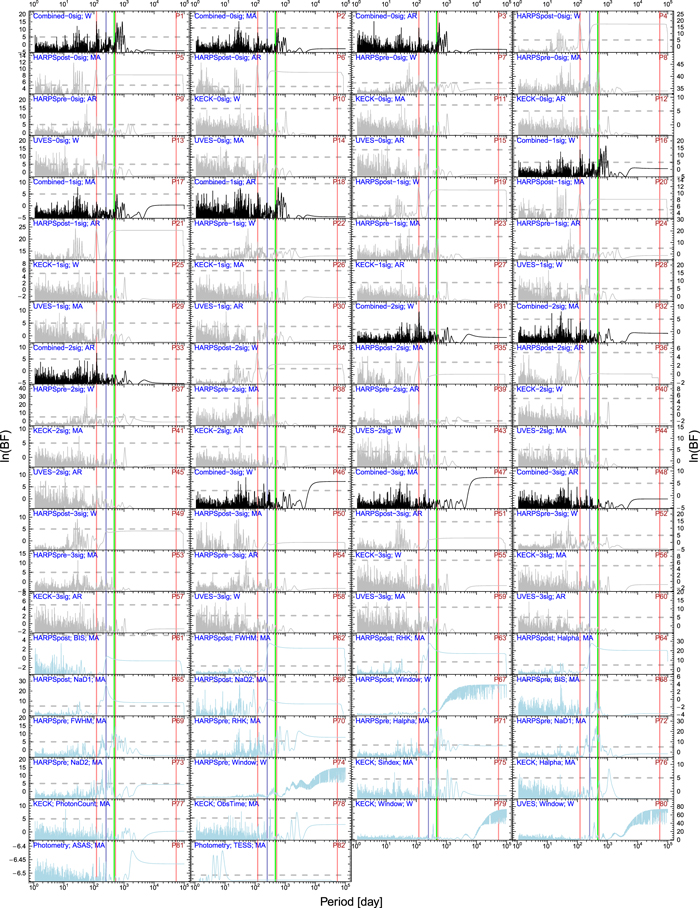
Figure 10. BFP for GJ 229A. The red lines denote signal periods of 52,900, 122 and 520 days, which are subtracted from the raw RV data subsequently to calculate the residual BFPs. The dark-blue lines denote the activity signal with a period of 278 days. The cyan line denotes the 471 day signal reported by T14. The BFPs for the individual data sets subtracted by three signals are not shown to simplify the figure.
Download figure:
Standard image High-resolution image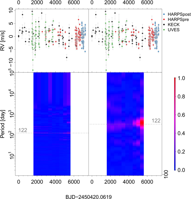
Figure 11. Moving periodogram for GJ 229A c. The 122 day signal is most significant in the HARPSpost data set, due to its high cadence.
Download figure:
Standard image High-resolution image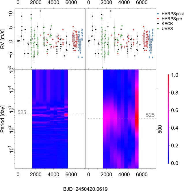
Figure 12. Moving periodogram for GJ 229A b. The annual aliases of the 525 day signal at periods of 215 and 1200 days are visible though not consistent over time.
Download figure:
Standard image High-resolution image
Figure 13. BFP for GJ 422. The red lines denote the signal at a period of 20.1 days while the dark-blue lines denote the activity signal with a period of 8.1 days. The green line denotes the 26 day signal found by T14.
Download figure:
Standard image High-resolution image
Figure 14. Moving periodogram for GJ 422 b. The annual aliases of the 20.1 day signal at periods of 19 and 21 days are visible though not consistent over time. The 20.1 day signal is not significant in recent epochs as in earlier epochs, due to low-cadence measurements in recent epochs.
Download figure:
Standard image High-resolution image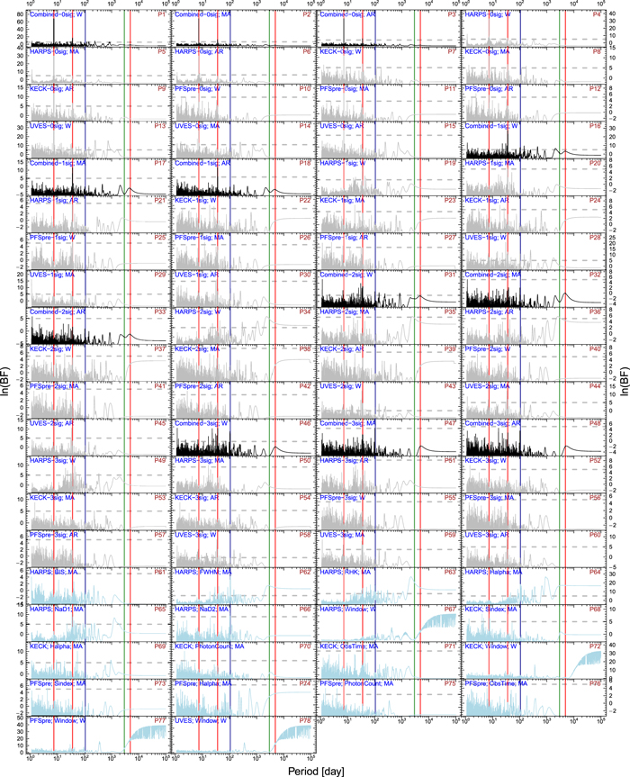
Figure 15. BFPs for GJ 433. The red lines denote signal periods of 7.37, 36.1, and 5090 days, which are subtracted from the raw RV data subsequently to calculate the residual BFPs. The dark-blue lines denote the activity signal with a period of 107 days.
Download figure:
Standard image High-resolution image
Figure 16. Moving periodogram for GJ 433 b. No annual aliases are visible. This signal is quite unique and consistent over time.
Download figure:
Standard image High-resolution image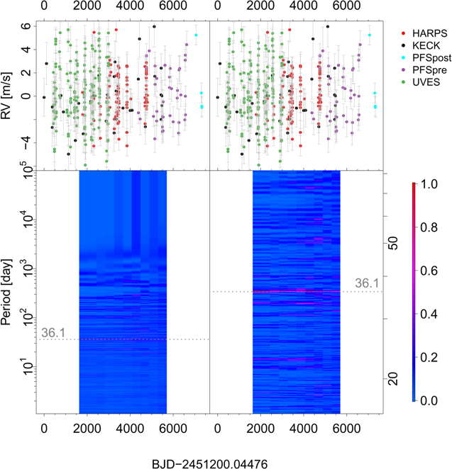
Figure 17. Moving periodogram for GJ 433 d. The annual aliases of the 36.1 day signal at periods of 33 and 40 days are visible though not consistent over time.
Download figure:
Standard image High-resolution image
Figure 18. BFPs for GJ 620. The red lines show the signals at periods of 7.65 and 27.2 days, which are subtracted from the raw RV data subsequently to calculate the residual BFPs.
Download figure:
Standard image High-resolution image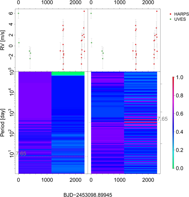
Figure 19. Moving periodogram for GJ 620 b. Considering the limited time span, the combined data set is equally divided into two chunks. The signal at a period of 7.65 days is significant in the HARPS set and is consistent with the UVES set.
Download figure:
Standard image High-resolution image
Figure 20. Moving periodogram for GJ 620 c. The signal at a period of 27.2 days is significant in the HARPS set and is consistent with the UVES set.
Download figure:
Standard image High-resolution image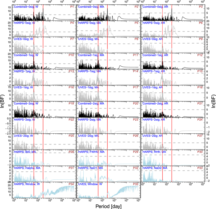
Figure 21. BFP for GJ 739. The red lines denote the signals at periods of 266 and 45.3 days, which are subtracted from the raw RV data subsequently to calculate the residual BFPs.
Download figure:
Standard image High-resolution image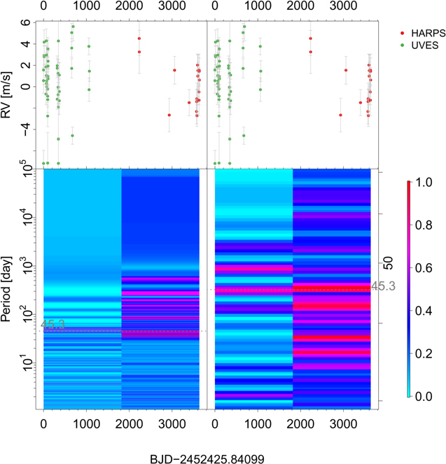
Figure 22. Moving periodogram for GJ 739 b. The signal at a period of 45.3 days is significant in the UVES set and is consistent with the HARPS set.
Download figure:
Standard image High-resolution image
Figure 23. Moving periodogram for GJ 739 c. The 266 day signal is strong both in the UVES and in the HARPS sets.
Download figure:
Standard image High-resolution image
Figure 24. BFP for GJ 911. The red lines denote the planetary signal at a period of 2.79 days. The dark-blue lines denote the activity signal at a period of 204 days.
Download figure:
Standard image High-resolution image
Figure 25. Moving periodogram for GJ 911. The annual aliases of the 2.79 day signal at periods of 2.81 and 2.77 days are visible.
Download figure:
Standard image High-resolution image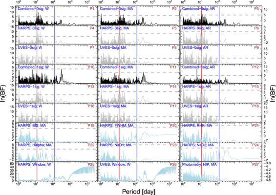
Figure 26. BFP for GJ 3082. The red lines denote the planetary signal at a period of 11.9 days. The dark-blue lines denote the activity signal at a period of 123 days. The P27 panel shows the BFP for the Hipparcos photometry (ESA 1997).
Download figure:
Standard image High-resolution image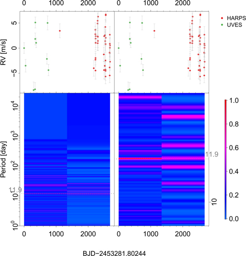
Figure 27. Moving periodogram for GJ 3082 b. The 11.9 day signal is consistently significant in HARPS and UVES sets.
Download figure:
Standard image High-resolution image4.3. Comments on Previous Planet Candidates
Based on our combined analysis of the other UVES targets, we comment on the planetary candidates reported in Table 4 of T14 as follows.
- 1.GJ 27.1 b. It is likely due to activity. The signals at periods of 31.8 and 10.3 days are identified in the combined UVES, Keck, and HARPS data. We show them in Figure 28 together with the 15.819 day signal reported by T14. The 31.8 day signal is found to be significant in the activity indices of BIS, FWHM, RHK, Hα, and NaD1 of the HARPS set, indicating an activity origin. The 15.8 day signal reported by T14 is nearly half of the activity signal, and strong powers around this period are seen in the BFPs for the FWHM (P14), (P15), and Hα (P16) of HARPS. The 10.3 day signal is not as significant as the 31.8 day signal in the BFPs for activity indices, although we still find strong powers around similar periods in the BFPs for the FWHM (P14) and NaD2 (P18) of HARPS. Considering that 31.8 days is significant and unique enough to disguise itself as a Keplerian signal, a comprehensive diagnosis of activity indices are necessary for reliable planet detections.
- 2.GJ 160.2 b. It is not identified. We do not find this signal through MCMC sampling of the posterior. As seen in Figure 29, no significant and unique signals are found in the red-noise BFPs for the combined data set (P2 and P3) despite strong powers in the white-noise BFPs (P1). Because the 5.2 day signal found by T14 is not visible in the new UVES set or in other data sets, it is unlikely to be Keplerian and might arise from data reduction.
- 3.GJ 682 b and c. They are probably due to activity. As seen in Figure 30, we did not find these two signals with periods of 17.48 and 57.32 days in the BFPs nor in the MCMC posterior samples. The signals with strong powers in the white-noise BFPs (P1) may be caused by correlated noise as we do not see them in red-noise BFPs (P2 and P3). Moreover, we find the 17.48 day signal to be significant in the BFP for the BIS of HARPS, indicating an activity origin. In the BFP for the FWHM of HARPS, we find another signal around 6.87 days to be significant. There is also a strong power around this period in the BFP for of HARPS. Thus, this signal might be caused by the differential rotation of the star.


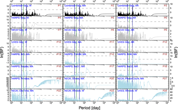
Figure 28. BFPs for GJ 27.1. The dark-blue lines show the most significant activity signals at a period of about 31.8 and 10.3 days. The green line shows the signal at a period of 15.819 days identified by T14.
Download figure:
Standard image High-resolution image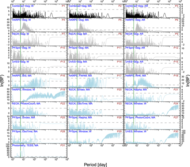
Figure 29. BFP for GJ 160.2. The green lines denote the signal at a period of 5.24 days found by T14.
Download figure:
Standard image High-resolution image
Figure 30. BFP for GJ 682. The dark-blue line denotes the activity signal at a period of 6.87 days, and the green lines denote the signals at 17.5 and 57.3 days reported by T14.
Download figure:
Standard image High-resolution image4.4. Dynamical Stability of GJ 180 and GJ 229
The angular momentum deficit (AMD) is typically used to study the dynamical stability of planetary systems (Laskar 2000; Laskar & Petit 2017). Although the AMD is efficient in generally assessing stability, AMD-unstable systems can be stabilized through mechanisms such as mean motion resonances (Laskar & Petit 2017). To avoid such caveats, we examine the orbital stability of the GJ 180 and GJ 229 systems with N-body integrations using the Mercury integration package (Chambers 1999).
For the two-planet GJ 180 system, we examine a grid of initial eccentricities e and masses mp for GJ 180 d spanning one standard deviation above and below the mean values listed in Table 2. The other elements for GJ 180 d and the mass and elements for GJ 180 b were held at their mean values. For each grid of mp and e values, we consider three inclinations for the system as a whole: 30°, 60°, and 90°. The masses for both planets were adjusted accordingly while keeping the planetary orbits coplanar. The integrations used a second-order mixed-variable symplectic (MVS) integrator with a step size of 0.7 days. The upper panel of Figure 31 shows a typical case with I = 90° and using the nominal mass and eccentricity for GJ 180 d. In this case, and all the other cases we considered, there is no indication of instability during the 1 Myr integration. The semimajor axes are almost constant, while the eccentricities undergo small, periodic oscillations. The orbits never approach each other. Although these integrations do not prove the system is stable, they clearly suggest that this is the case.

Figure 31. One sample of the dynamical simulations for GJ 180 (upper) and GJ 229 (lower) over one million years. The three curves of each color show the apastron distance, semimajor axis, and periastron distance for a planet. In the upper panel, the red curves represent GJ 180 b, and the green curves represent GJ 180 d. In the lower panel, the red, green, and blue curves represent GJ 229A c, GJ 229 b, and GJ 229B, respectively.
Download figure:
Standard image High-resolution image
For the GJ 229 system, we included planets GJ 229A c and GJ 229A b as well as the likely brown dwarf GJ 229B. We examined a grid of values for the e and M of GJ 229A c spanning one standard deviation above and below the mean values given in Table 2, holding all other quantities fixed at their nominal values. For each grid, we considered two inclinations for the system such that the masses of each object were either 10 or 20 times the nominal values for an edge-on system (corresponding to inclinations of about 5 7 and 29 respectively). These choices reflect the fact that GJ 229B is probably a brown dwarf, which suggests that the system is nearly face-on to us. The orbits of the planets and brown dwarf were assumed to be coplanar. The integrations used an MVS integrator with a step size of 4 days. The lower panel of the Figure 31 shows a typical case with I = 57 and the nominal mass and eccentricity for GJ 229A c. As with GJ 180, the orbits show no sign of instability over 1 Myr, and this was true for all the cases we considered here.
5. Conclusion
We identify 16 planet candidates orbiting nine nearby M dwarfs from the combined analysis of the UVES, HIRES/Keck, HARPS, and PFS velocity data sets. Among these candidates, GJ 173 b, GJ 180 d, GJ 229A c, GJ 422 b, GJ 433 d, and GJ 3082 b are five new planets corresponding to RV signals that are statistically significant, robust to the choice of noise model, unique and consistent over time. Thus, they are likely real planets. We confirm three previously reported planet candidates and find eight planet candidates which need additional observations to be further confirmed.
In the new sample of candidates, two temperate super-Earths, GJ 180 d and GJ 229A c, are located in the HZs of their host stars. Due to their proximity, the separation between the host stars and the potentially habitable planets is in these systems is 25 mas and 59 mas, respectively. These are good candidates for future direct imaging by future facilities.
GJ 433 c is a cold super-Neptune candidate located in a mass–period regime rarely explored. It is separated from its host star by about 05 and thus is a good candidate for direct imaging. A comprehensive RV survey of these planets would help us better understand Neptune-like planets.
Among the 16 candidates, 4 planets have been reported by T14 and GJ 229B, a T-type brown dwarf, has been discovered by Nakajima et al. (1995) through direct imaging. With updated UVES and HARPS data combined with Keck and PFS, we provide improved constraints on the orbits of these planets. However, we fail to confirm GJ 27.1 b, GJ 160.2 b, and GJ 682 b and c reported by T14, probably due to our use of updated UVES data and more RV sets. Some of these signals probably have an activity origin through our diagnosis of the periodograms for activity indices.
There are five multiple-planet systems. GJ 180, GJ 620, and GJ 739 each hosts two planets. GJ 229 and GJ 433 each hosts three planets.11 These planets are likely stable because their orbits are not eccentric and are well separated. In particular, we examine the stability of GJ 229 and GJ 180 systems by simulating the orbits of their planets over one million years. We find that all planets in these two systems are stable, suggesting long-term stable orbits of the two temperate planets GJ 229A c and GJ 180 d.
Our detection of these Keplerian signals demonstrates the value of a combined analysis of multiple RV data sets to extend the time baseline and avoid instrumental bias. We also highlight the importance of the moving periodogram in the confirmation of signals. The time-consistent uniqueness and significance of GJ 173 b (Figure 6), GJ 180 d (Figure 9), GJ 229A c (Figure 11), GJ 433 b (Figure 16), and GJ 433 d (Figure 17) are well presented by the moving periodograms. Hence,we recommend moving periodograms as a tool for signal visualization. Our identification of false positives through BFPs of activity indices demonstrate an essential role of comprehensive periodogram analysis in planet discoveries. Our work is based on an updated data reduction of the UVES data collected in 2009. This demonstrates the ongoing necessity of better analysis of archived RV data to reveal small signals. Because we cannot go back in time, these data represent our earliest epoch for future discoveries.
This work has made use of data from the European Space Agency (ESA) mission Gaia (https://www.cosmos.esa.int/gaia), processed by the Gaia Data Processing and Analysis Consortium (DPAC, https://www.cosmos.esa.int/web/gaia/dpac/consortium). Funding for the DPAC has been provided by national institutions, in particular the institutions participating in the Gaia Multilateral Agreement. This research has also made use of the Keck Observatory Archive (KOA), which is operated by the W. M. Keck Observatory and the NASA Exoplanet Science Institute (NExScI), under contract with the National Aeronautics and Space Administration. This research has also made use of the services of the ESO Science Archive Facility, NASA's Astrophysics Data System Bibliographic Service, and the SIMBAD database, operated at CDS, Strasbourg, France. Support for this work was provided by NASA through Hubble Fellowship grant HST-HF2-51399.001 awarded by the Space Telescope Science Institute, which is operated by the Association of Universities for Research in Astronomy, Inc., for NASA, under contract NAS5-26555. The authors acknowledge the years of technical support from LCO staff in the successful operation of PFS, enabling the collection of the data presented in this paper.
Software: R package magicaxis (Robotham 2016), fields,12 minpack.lm,13 nortest,14 aTSA.15
Appendix A: Tests for Priors
To test the sensitivity of parameter inference and model selection to eccentricity priors, we compare the parameter values and ln(BF) for the semi-Gaussian eccentricity prior with standard deviation of 0.2 (used in this work) and 0.4 in Table 3.
Table 3. Sensitivity of Parameter Inference and Model Selection to Eccentricity Priors
| Targets |

|

|
||||
|---|---|---|---|---|---|---|
| P (days) | K (m s−1) | e | P (days) | K (m s−1) | e | |
| GJ 180 d |

|

|

|

|

|

|
| GJ 229A c |

|

|

|

|

|

|
| GJ 422 b |

|

|

|

|

|

|
| GJ 433 d |

|

|

|

|

|

|
| GJ 3082 b |

|

|

|

|

|

|
Note. The optimal values of parameters correspond to the MAP solution, and their uncertainties are determined at the 10% and 90% quantiles of the MCMC posterior samples.
Download table as: ASCIITypeset image
Appendix B: Tests for Residuals
We test the normality, autocorrelation, and stationarity of residuals using the Anderson–Darling (AD) test (Anderson & Darling 1952), the Ljung–Box (LB) test (Box & Pierce 1970; Ljung & Box 1978), and the Augmented Dickey–Fuller (DF) (Dickey & Fuller 1979), respectively. Augmented DF tests of various types with lags of less than four show a p-value of ≤0.01. The DF tests for larger time lags show a slightly higher p-value, though it is still less than 0.05. However, this low p-value may not suggest nonstationarity because DF is typically applied to regularly spaced time series. To test this, we fit a linear trend to each residual and apply the DF test to the new residuals without any lag (i.e., traditional DF test). The p-value is still ≤0.01 and thus suggests a linear trend, although the best-fit linear trend is subtracted from the residual if there is any. Hence, the DF test is not appropriate for testing the stationarity of irregularly spaced time series.
We report the statistic and p-value for the AD and LB tests for each target in Table 4. The AD normality tests suggest that the RV residual for GJ 173 does not follow a Gaussian distribution, suggesting potential signals in the residuals. This is consistent with the two strong signals around periods of 20 and 60 days shown in the residual BFPs (see P13–P15 of Figure 5). The AD tests for the other residuals also show relatively low p-values, due to potential signals in RV residuals. Because the moving average model used in this study is stochastic and cannot model insignificant periodic signals, we expect considerable time-correlated noise or signal over long timescales in RV residuals.
Table 4. Statistic and p-value of the Anderson–Darling and Ljung–Box Tests for the Residuals
| Target | AD Statistic | AD p-value | LB Statistic | LB p-value |
|---|---|---|---|---|
| GJ 173 | 1.3 | 0.0027 | 4.5 | 0.033 |
| GJ 180 | 0.52 | 0.18 | 0.98 | 0.32 |
| GJ 229A | 3.1 |

|
0.93 | 0.33 |
| GJ 422 | 2.4 |

|
0.34 | 0.56 |
| GJ 433 | 0.46 | 0.26 | 1.6 | 0.21 |
| GJ 620 | 0.67 | 0.073 | 0.68 | 0.41 |
| GJ 739 | 0.86 | 0.026 | 0.32 | 0.57 |
| GJ 911 | 1.9 |

|
0.0072 | 0.93 |
| GJ 3082 | 0.2 | 0.88 | 6.3 | 0.012 |
Download table as: ASCIITypeset image
The p-values of the LB tests for GJ 180, GJ 229A, GJ 422, GJ 433, GJ 620, GJ 739, and GJ 911 are high, suggesting insignificant autocorrelation in residuals. However, the LB tests for GJ 173 and GJ 3082 have low p-values, indicating considerable autocorrelation. For these two targets, we model the noise using white-noise models according to the Bayesian model selection scheme introduced in Section 3.2. Thus, in the RV residuals, we expect to find time-correlated noise, which is not significant enough to be modeled by the MA model.
Footnotes
- *
This paper includes data gathered with the 6.5 m Magellan Telescopes located at the Las Campanas Observatory, Chile.
- 8
- 9
- 10
- 11
Here we count GJ 229B as a planet.
- 12
- 13
- 14
- 15