


Abstract
The coalescence of a binary neutron star gives rise to electromagnetic emission, known as a kilonova, that is powered by radioactive decays of r-process nuclei. Observations of a kilonova associated with GW170817 provide a unique opportunity to study heavy element synthesis in the universe. However, the atomic data of r-process elements are not yet complete enough to decipher the light curves and spectral features of kilonovae. In this paper, we perform extended atomic calculations of neodymium (Nd, Z = 60) to study the impact of the accuracy in atomic calculations on astrophysical opacities. By employing multiconfiguration Dirac–Hartree–Fock and relativistic configuration interaction methods, we calculate the energy levels and transition data of electric dipole transitions for Nd ii, Nd iii, and Nd iv ions. Compared with previous calculations, our new results provide better agreement with the experimental data. The energy level accuracies achieved in the present work are 10%, 3%, and 11% for Nd ii, Nd iii, and Nd iv, respectively, compared to the NIST database. We confirm that the overall properties of the opacity are not significantly affected by the accuracies of the atomic calculations. The impact on the Planck mean opacity is up to a factor of 1.5, which affects the timescale of kilonovae by at most 20%. However, we find that the wavelength-dependent features in the opacity are affected by the accuracies of the calculations. We emphasize that accurate atomic calculations, in particular for low-lying energy levels, are important to provide predictions of kilonova light curves and spectra.
Export citation and abstract BibTeX RIS
1. Introduction
On 2017 August 18, the first observation of gravitational waves (GWs) from a neutron star (NS) merger was achieved (GW170817, Abbott et al. 2017a). In addition to GWs, electromagnetic (EM) counterparts across the wide wavelength range were also observed (Abbott et al. 2017b). In particular, intensive observations of the optical and near-infrared (NIR) counterpart (SSS17a, also known as DLT17ck or AT2017gfo) have been performed and dense photometric and spectroscopic data were obtained (Andreoni et al. 2017; Arcavi et al. 2017; Chornock et al. 2017; Coulter et al. 2017; Cowperthwaite et al. 2017; Díaz et al. 2017; Drout et al. 2017; Evans et al. 2017; Kasliwal et al. 2017; Kilpatrick et al. 2017; Lipunov et al. 2017; McCully et al. 2017; Nicholl et al. 2017; Pian et al. 2017; Shappee et al. 2017; Siebert et al. 2017; Smartt et al. 2017; Soares-Santos et al. 2017; Tanvir et al. 2017; Tominaga et al. 2018; Troja et al. 2017; Utsumi et al. 2017; Valenti et al. 2017). SSS17a shows that the characteristic properties are quite different from those of supernovae. The optical light curves decline rapidly, while NIR light curves evolve more slowly. The spectra show featureless, broad-line features implying a high expansion velocity. These properties are broadly consistent with theoretically suggested kilonova or macronova emission from NS mergers (Li & Paczyński 1998; Kulkarni 2005; Metzger et al. 2010).
A kilonova is EM emission powered by radioactive decay energy of the r-process nuclei that are newly synthesized in NS mergers (see Rosswog 2015; Fernández & Metzger 2016; Tanaka 2016; Metzger 2017, for reviews). The timescale, luminosity, and color of the emission are mainly determined by the mass and velocity of the ejecta and opacities in the ejecta. Among r-process elements, lanthanide elements have high optical and NIR opacities (Kasen et al. 2013; Tanaka & Hotokezaka 2013). Therefore, if the ejecta include lanthanide elements, the emission becomes red and faint. On the other hand, if the ejecta are free from lanthanide elements, the emission is blue and bright (Metzger & Fernández 2014; Kasen et al. 2015; Tanaka et al. 2018).
In fact, SSS17a shows both blue and red components, which implies that there are multiple components with different lanthanide content. This suggests the production of a wide range of r-process elements (Kasen et al. 2017; Tanaka et al. 2017; Rosswog et al. 2018). This is also consistent with expectations from numerical relativity simulations (see e.g., Perego et al. 2017; Shibata et al. 2017). The ejecta mass to explain the luminosity of SSS17a is about  . Although it is still unclear if the r-process yields from NS mergers are consistent with the solar ratios, NS mergers may be the dominant site for the r-process elements in the universe (Hotokezaka et al. 2018; Rosswog et al. 2018).
Although the observed properties can be explained by the kilonova scenario, the physics included in current kilonova simulations is not yet perfect. In particular, the atomic data of r-process elements are not complete: so far, calculated data are available only for a limited number of r-process elements (Kasen et al. 2013, 2017; Fontes et al. 2017; Tanaka et al. 2018; Wollaeger et al. 2018). Even when the data are available, they are almost entirely based on theoretical calculations, and the derived energy levels often deviate from experimental data by up to ∼30% (note that experimental data are also insufficient). It is not yet clear if these issues have systematic impacts on the opacities as well as the properties of kilonova.
In this paper, we study the impacts of the accuracies in atomic calculations on the opacities by performing extensive, accurate calculations. For this purpose, we choose a lanthanide element, neodymium (Nd, Z = 60), which has also been studied by Kasen et al. (2013), Fontes et al. (2017), and Tanaka et al. (2018). We focus on singly to triply ionized Nd, for which accurate calculations are possible with the multiconfiguration Dirac–Hartree–Fock (MCDHF) method. In Sections 2 and 3, we describe the methods and strategies of our atomic calculations. In Section 4, we show and evaluate the results of our atomic calculations. In Section 5, we show the impact of the accuracy of the atomic calculations on the astrophysical opacities. Finally, we provide a summary in Section 6.
2. Methods
2.1. Computational Procedure
The GRASP2K package (Jönsson et al. 2013) is based on the MCDHF and relativistic configuration interaction (RCI) methods, and takes into account the transverse photon interaction (Breit interaction) and quantum electrodynamic (QED) corrections (Grant 2007; Fischer et al. 2016).
The MCDHF method used in the present work is based on the Dirac–Coulomb Hamiltonian

where VN is the monopole part of the electron–nucleus Coulomb interaction,  and β are the 4 × 4 Dirac matrices, and c is the speed of light in atomic units. The atomic state functions (ASF) were obtained as linear combinations of symmetry-adapted configuration state functions (CSFs)

Here, J and M are the angular quantum numbers and P is parity.  denotes other appropriate labeling of the CSF j such as, for example, the orbital occupancy and coupling scheme. Normally, the label
  of the atomic state function is the same as the label of the dominant CSF. The CSFs are built from products of one-electron Dirac orbitals. Based on a weighted energy average of several states, the so-called extended optimal level (EOL) scheme (Dyall et al. 1989), both the radial parts of the Dirac orbitals and the expansion coefficients were optimized to self-consistency in the relativistic self-consistent field procedure. Note that because accurate calculations with the MCDHF method are much more difficult for neutral atoms than for ions (Grant 2007), we focus on ionized Nd.
For these calculations, we used the spin-angular approach (Gaigalas & Rudzikas 1996; Gaigalas et al. 1997), which is based on the second quantization in coupled tensorial form, on the angular momentum theory in three spaces (orbital, spin, and quasispin) and on the reduced coefficients of fractional parentage. It allowed us to study configurations with open f -shells without any restrictions.
In subsequent RCI calculations the Breit interaction
was included in the Hamiltonian. The photon frequencies  , used for calculating the matrix elements of the transverse photon interaction, were taken as the difference of the diagonal Lagrange multipliers associated with the Dirac orbitals (McKenzie et al. 1980). In the RCI calculation the leading QED corrections, self-interaction and vacuum polarization, were also included.
In the present calculations, the ASFs were obtained as expansions over jj-coupled CSFs. To provide the LSJ labeling system, the ASFs were transformed from a jj-coupled CSF basis into an LSJ-coupled CSF basis using the method provided by Gaigalas et al. (2017).
2.2. Computation of Transition Parameters
The evaluation of radiative transition data (transition probabilities, oscillator strengths) between two states,  and
and  , built on different and independently optimized orbital sets, is non-trivial. The transition data can be expressed in terms of the transition moment, which is defined as

where  is the transition operator. For electric dipole and quadrupole (E1 and E2) transitions there are two forms of the transition operator: the length (Babushkin) and velocity (Coulomb) forms, which for the exact solutions of the Dirac-equation give the same value of the transition moment (Grant 1974). The quantity dT, characterizing the accuracy of the computed transition rates, is defined as

where  and
and  are transition rates in length and velocity forms.
The calculation of the transition moment breaks down the task of summing up reduced matrix elements between different CSFs. The reduced matrix elements can be evaluated using standard techniques assuming that both the left and right CSFs formed from the same orthonormal set of spin-orbitals. This constraint is severe, because a high-quality and compact wave function requires orbitals optimized for a specific electronic state; see, for example Fritzsche & Grant (1994). To get around the problem of having a single orthonormal set of spin-orbitals, the wave function representations of the two states  and
and  were transformed in such a way that the orbital sets became biorthonormal (Olsen et al. 1995). Standard methods were then used to evaluate the matrix elements of the transformed CSFs.
3. Schemes of the Calculations
3.1. Active Space Construction
A summary of the MCDHF and RCI calculations for each ion is given in Table 1. The description, which explains how these calculations were done, is given below. As a starting point, DHF calculations were performed in the EOL scheme for the states of the ground configuration. The wave functions from these calculations were taken as the initial ones to calculate even and odd states of multireference (MR) configurations. The set of orbitals belonging to these MR configurations is referred to as 0 layer (0L).
Table 1. Summary of Active Space Construction
| Ion | Ground | MR set | Active Space | Number of Levels | NCSFs | |||
|---|---|---|---|---|---|---|---|---|
| conf. | Even | Odd | Even | Odd | Even | Odd | ||
| Strategies A, B.1 | ||||||||
| Nd ii |

|
 , , 
|
 , , 
|

|
3 890 | 2 998 | 24 568 | 23 966 |
 , , 
|

|
|||||||
| Additional configuration in Strategy B.2 | ||||||||
 , , 
|
 , , 
|
|
1 039 | 1 013 | 468 652 | 468 029 | ||

|
||||||||
| Strategy C | ||||||||
 , , 
|
 , , 
|
|
3 270 | 2 813 | 188 357 | 113 900 | ||
 , , 
|

|
|||||||
| Strategies A, B | ||||||||
| Nd iii |

|
 , , 
|
 , , 
|

|
1 020 | 468 | 400 440 | 259 948 |
 , , 
|
||||||||
| Strategy C | ||||||||
 , , 
|
 , , 
|

|
747 | 706 | 844 637 | 559 294 | ||
 , , 
|
 , , 
|
|||||||
 , , 
|
||||||||
| Strategy C with 5p,5s | ||||||||
 , , 
|
 , , 
|

|
747 | 706 | 900 904 | 586 850 | ||
 , , 
|
 , , 
|
|||||||
 , , 
|
||||||||
| Strategy A | ||||||||
| Nd iv |

|
 , , 
|
 , , 
|

|
131 | 110 | 33 825 | 26 590 |
| Strategy B | ||||||||
 , , 
|
 , , 
|
|
1 068 | 465 | 1 445 481 | 587 774 | ||

|

|
|||||||
| Strategy B with 5s | ||||||||
 , , 
|
 , , 
|

|
1 068 | 465 | 1 474 463 | 603 827 | ||

|

|
|||||||
Download table as: ASCIITypeset image
Unless stated otherwise, the inactive core of each ion used in the present calculations is [Xe]. The CSF expansions for the states of each parity were obtained by allowing single (S) and double (SD) substitutions from the MR configurations up to active orbital sets (see Table 1). The configuration space was increased step-by-step with increasing the number of layers (L). The orbitals of previous layers were held fixed and only the orbitals of the newest layer were allowed to vary. For example, the scheme used to increase the active spaces of the CSFs for Nd iii ion (in Strategy A) is presented below:
-
 = {6s, 6p, 5d},
 -
+ {7s, 7p, 6d, 5f, 5g},
-
+ {8s, 8p, 7d, 6f, 6g, 6h},
-
+ {9s, 9p, 8d, 7f, 7g, 7h}.


The MCDHF calculations were followed by RCI calculations, including the Breit interaction and leading QED effects. The number of CSFs in the final even and odd state expansions distributed over the different J symmetries is presented in Table 1.
3.2. Strategies for the Nd ii ion
Four strategies were tested for Nd ii ion. All of them were computed in the active space described in the Table 1. For Strategy A, the starting point DHF calculations were performed in the EOL scheme for the states of the ground configuration  . The wave functions from these calculations were taken as the initial ones to calculate the even and odd states of MR configurations. The set of orbitals belonging to these MR configurations is referred to as 0 layer (0L). The active spaces were generated as is presented in Table 1.
For Strategy B.1 the starting point was a computation of the wave functions for the core  . Wave functions were computed in the neutral system of Nd i - ground state
  . Then,
  was computed: the core shells were frozen and only
  and
and  shells of the configurations of MR listed in Table 1 were computed. Even and odd states were computed together. Later, wave functions were optimized separately for states of different parities in the
  .
.  and the next active space were generated by SD substitutions from shells
  .
.
In Strategy B.2 the configurations of the Rydberg states listed in Table 1 were added to the MR list; therefore, the first active set included subshells that were larger by one principal quantum number. Then, the first active space of Strategy B.2 was  .
.
In Strategy C, computations were performed for each configuration separately. For configurations  ,
,  and
and  SD substitutions were allowed from
  (where
  ) shells into the
  and S into the
  . For configurations
  ,
,  ,
,  , and
, and  only S substitutions were allowed. Radial wave functions up to the
  orbital were taken from the ground configuration for these configurations. The Breit interaction and leading QED effects are included in RCI computations.
3.3. Strategies for the Nd iii ion
After  the even and odd states were calculated separately in Strategy A. For the Nd iii ion calculations Strategy B was also applied. Strategy B differs from Strategy A in that virtual orbitals for odd parity were taken from even parity states instead of varying them in layer 1 and higher layers.
In Strategy C, compared to Strategy A additional configurations,  ,
,  (odd parity) and
  ,
,  (even parity), were added to the MR set. In Strategy C with
  just RCI calculations were performed. The wave functions were taken from Strategy C and configurations with S substitutions from
  and
and  shells to
  shells were added additionally in the active space.
3.4. Strategies for the Nd iv ion
In Strategy B, compared to Strategy A, additional configurations,  (odd parity) and
  (even parity), were added to the MR set. The ASFs for even and odd parities were constructed such that SD substitutions were allowed from the
  shells up to active orbital sets and S substitution from the
  shell to
  shells. In Strategy B, with 5s just RCI calculations were performed. The wave functions were taken from Strategy B and configurations with S substitutions from
  shells to
  shells were added additionally in the active space.
4. Results
4.1. Nd ii
A part of all computed excitation energies for Nd ii are listed in Table 2. These data were compared with the NIST database by evaluating the relative difference  . The energy levels computed with Breit interaction and QED effects are presented in columns marked by *. Levels with changed notations are given in Table 3.
Table 2. Computations of Energy Values (in cm−1) of Nd ii by Increase of the Active Space Performed, Applying Strategies A, B.1, B.2, and C and Their Comparison with the NIST Database (in %)
| Strategy A | Strategy B.1 | Strategy B.2 | Strategy C | ||||
|---|---|---|---|---|---|---|---|
| Config. | Term | J | NIST |

|
|
|

|

|

|
7/2 | 0.000 | ||||

|
9/2 | 513.330 | −14/−9 | −16/−10/−2/−10 | −9/−9/−9 | −6/−7 | |

|
11/2 | 1470.105 | −5/−3 | −6/−3/8/−3 | −0/0/−3 | 5/4 | |

|

|
9/2 | 1650.205 | −13/−8 | −15/−9/−3/−8 | −8/−7/−8 | −8/−8 |

|

|
13/2 | 2585.460 | −5/−3 | −4/−3/9/−3 | 1/1/−3 | 6/6 |

|

|
11/2 | 3066.755 | −9/−6 | −10/−6/2/−6 | −4/−4/−6 | −1/−2 |

|

|
15/2 | 3801.930 | −5/−4 | −5/−4/8/−4 | 0/0/−4 | 6/6 |

|

|
11/2 | 4437.560 | −13/−7 | −38/−3/2/−3 | −2/−3/1 | 4/9 |

|

|
13/2 | 4512.495 | −9/−6 | −9/−6/0/−6 | −4/−3/−6 | 0/0 |

|

|
17/2 | 5085.640 | −6/−5 | −6/−5/7/−5 | −1/−1/−5 | 6/6 |

|

|
13/2 | 5487.655 | −10/−5 | −30/−2/1/−2 | −1/−1/1 | 6/10 |

|

|
15/2 | 5985.580 | −9/−7 | −9/−7/4/−7 | −4/−4/−7 | 1/1 |

|

|
9/2 | 6005.270 | −12/−7 | −36/−4/−3/−4 | −5/−5/−2 | −6/−1 |

|

|
15/2 | 6637.430 | −8/−4 | −24/−1/3/−1 | 0/0/0 | 7/10 |

|

|
11/2 | 6931.800 | −10/−6 | −31/−3/−1/−3 | −3/−3/−2 | −3/1 |

|

|
7/2 | 7524.735 | −24/−19 | −50/−17/−16/−17 | −19/−19/−15 | −16/−1 |

|

|
17/2 | 7868.910 | −7/−3 | −20/−1/4/−1 | 1/1/0 | 7/10 |

|

|
13/2 | 7950.075 | −9/−5 | −27/−3/1/−3 | −3/−3/−2 | −2/2 |

|

|
13/2 | 8009.810 | 0/−12 | −7/−11/−6/−14 | −7/−10/−14 | 32/32 |

|

|
9/2 | 8420.320 | −21/−16 | −43/−14/−12/−14 | −15/−16/−13 | −13/−9 |

|

|
3/2 | 8716.445 | −20/−15 | −42/−13/−12/−13 | −16/−16/−13 | −14/−11 |

|
5/2 | 8796.365 | −23/−17 | −46/−15/−14/−15 | −19/−19/−15 | −17/−14 | |

|

|
15/2 | 9042.760 | −8/−5 | −24/−3/2/−3 | −2/−2/−2 | 0/3 |

|

|
19/2 | 9166.210 | −6/−3 | −17/−1/5/−1 | 1/1/−1 | 7/10 |

|

|
7/2 | 9198.395 | −24/−18 | −46/−16/−15/−16 | −19/−19/−15 | −17/−14 |

|

|
11/2 | 9357.910 | −18/−14 | −39/−12/−10/−12 | −13/−13/−11 | −10/−7 |

|

|
15/2 | 9448.185 | −1/−12 | −9/−12/−6/−14 | −8/−11/−14 | 29/29 |

|

|
5/2 | 9674.835 | −28/−22 | −55/−20/−20/−30 | −24/−25/−19 | −23/−19 |

|

|
11/2 | 10054.195 | −71/−50 | −73/−77/73/−79 | −73/−75/−79 | 1/1 |

|

|
9/2 | 10091.360 | −70/−51 | −71/−75/−101/−77 | −71/−73/−77 | −1/0 |

|

|
17/2 | 10194.805 | −8/−5 | −21/−3/2/−3 | −2/−2/−3 | 1/3 |

|

|
1/2 | 10256.040 | −37/−37 | −38/−37/−36/−35 | −37/−35/−35 | −28/−28 |

|

|
13/2 | 10337.100 | −17/−13 | −35/−11/−8/−11 | −12/−12/−11 | −8/−6 |

|

|
3/2 | 10439.225 | −37/−36 | −37/−48/−36/−35 | −36/−34/−35 | −28/−27 |

|

|
21/2 | 10516.790 | −6/−3 | −15/−1/5/−1 | 0/0/−2 | 7/9 |

|

|
7/2 | 10666.780 | −25/−20 | −36/−19/−17/−18 | −11/−11/−8 | −19/−16 |

|

|
11/2 | 10720.295 | −67/−82 | −82/−82/−69/−75 | −69/−80/−75 | −3/−2 |

|

|
5/2 | 10786.775 | −36/−36 | −37/−50/−35/−34 | −35/−47/−34 | −27/−27 |
Note. The "*" energy levels were computed with Breit interaction and QED effects are presented.
Download table as: ASCIITypeset image
Table 3. NIST Recommended Energy Level Notations Changed by the Authors for Nd ii
| NIST label | Our label |
|---|---|
|
|
|
|
Download table as: ASCIITypeset image
Note that the energy levels of Nd ii are also provided by Wyart (2010). They interpreted 596 levels of odd configurations ( ,
,  ,
,  ,
,  and
and  ) in a semi-empirical way following the Racah-Slater parametric method, using the Cowan computer codes. In their method, the radial parameters obtained in a least-squares fit were compared with Hartree–Fock (HFR) ab initio integrals. Because of this, the obtained energy levels naturally have very small disagreement with NIST values, and therefore are not presented in this paper.
The energy levels for each configuration are compared with NIST in Figure 1. Among the different strategies, Strategy C  gives the best agreement with the NIST database. The averaged difference between our computed data and the NIST presented values is 10%. This is a significant improvement compared with Strategy A
  (blue in Figure 1), which was used to compute the opacity of the neutron star mergers in Tanaka et al. (2018). The averaged difference with / NIST is 22% in Strategy A
  . For comparison with the NIST, the expression
  was used, where N is the number of compared levels.

Figure 1. Energy levels for configurations of Nd ii compared with the NIST data. Black represents NIST data, the column in red contains our computed energy levels in Strategy C  , and the blue data are based on Strategy A
  (used in Tanaka et al. 2018). The numbers above the red and blue columns are the averaged disagreements in percent for the levels of each configuration, compared with the NIST database.
Download figure:
Standard image High-resolution imageFigure 2 shows the distribution of the energy level number over the relative difference compared to NIST for Strategy A in active space  . For strategies A, B.1, and B.2, in all active spaces the distributions look very similar. For Strategy C, in
  (see Figure 2) a normal distribution with a smaller
  range is observed.
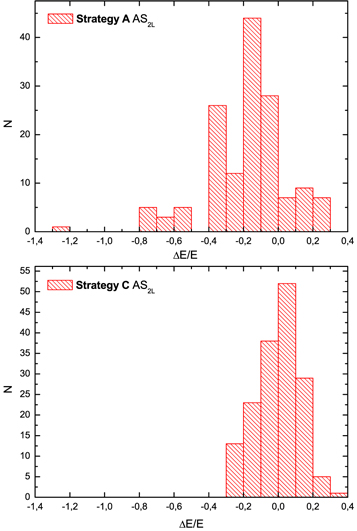
Figure 2. Distribution of energy levels (N) according to the disagreement with the NIST database for Nd ii using Strategy A and Strategy C in  .
.
Download figure:
Standard image High-resolution imageThe energy data computed in Strategy C at layer 2 are given in machine-readable format in Table 9. This includes number, label, J and P values, and energy value. The transitions data obtained from Strategy C at layer 2 are given in machine-readable form in Table 10. This includes identification of upper and lower levels in LSJ coupling, transition energy, wavelength, line strength, weighted oscillator strength, and transition probabilities in length form.
4.2. Nd iii
The results of the energy levels for Nd iii obtained from applying Strategies A, B C, and C with 5p, 5s are compared with the NIST database and presented in Table 4. Among the strategies, Strategy C with 5p, 5s gives the best agreement with the NIST database, although the number of available levels is smaller than that in the case of Nd ii. All the energy levels and transition data obtained from this strategy are listed in machine-readable form in Tables 11 and 12. Figure 3 shows a comparison of the energy levels with the NIST database. The averaged difference between our calculations with Strategy C with 5p, 5s  and the NIST data is 3%. For comparison, the difference for the case of Strategy B
  , which was used by Tanaka et al. (2018), is 5% (blue in Figure 3).
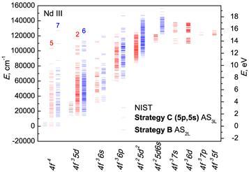
Figure 3. Energy levels for configurations of Nd iii compared with NIST data. Black represents NIST data, red represents our computed energy levels in Strategy C (5p,5s)  , and blue data are based on Strategy B
  . The numbers above the red and blue columns are averaged disagreements in percent for levels of each configuration, compared with the NIST database.
Download figure:
Standard image High-resolution imageTable 4. Comparison of Our Energy Levels to the NIST Database (in %) of Nd iii by Increase of the Active Space Performed, Applying Strategies A, B, C, and C with 5p, 5s
| Strategy A | Strategy B | Strategy C | Strategy C (5p,5s) | ||||
|---|---|---|---|---|---|---|---|
| Config. | Term | J | NIST |

|

|

|

|

|

|
4 | 0.0 | ||||
| 5 | 1137.8 | 8.8/8.5/8.4 | 8.7/8.5/8.4 | 8.8/8.5/8.4 | 6.1/5.9/5.7 | ||
| 6 | 2387.6 | 7.9/7.7/7.7 | 7.9/7.7/7.7 | 7.9/7.8/7.7 | 5.4/5.3/5.2 | ||
| 7 | 3714.9 | 7.0/7.0/7.0 | 7.0/7.0/7.0 | 7.1/7.1/7.0 | 4.7/4.7/4.6 | ||
| 8 | 5093.3 | 6.2/6.2/6.3 | 6.2/6.2/6.3 | 6.3/6.4/6.3 | 4.0/4.1/4.1 | ||

|

|
5 | 15262.2 | 7.2/11.6/7.4 | 6.8/6.4/6.8 | 7.5/7.0/6.8 | 1.4/1.1/0.9 |
| 6 | 16938.1 | 7.0/11.0/7.1 | 6.7/6.3/6.6 | 7.4/6.8/6.6 | 1.9/1.5/1.3 | ||
| 7 | 18656.3 | 6.6/10.2/6.7 | 6.4/6.0/6.3 | 7.0/6.4/6.2 | 2.1/1.7/1.5 | ||

|

|
4 | 18883.7 | −2.7/2.1/−1.2 | −3.5/−2.8/−1.8 | −2.3/−1.7/−1.7 | 0.5/0.9/0.9 |

|

|
3 | 19211.0 | −5.3/−0.5/−3.8 | −6.2/−5.1/−4.3 | −5.0/−4.2/−4.2 | −3.7/−2.8/−2.8 |
| 4 | 20144.3 | −3.2/1.3/−1.8 | −3.9/−3.1/−2.4 | −2.9/−2.3/−2.3 | −2.3/−1.6/−1.6 | ||

|

|
5 | 20388.9 | −1.9/2.5/−0.6 | −2.6/−2.1/−1.1 | −1.5/−1.1/−1.1 | 0.5/0.9/0.9 |

|

|
8 | 20410.9 | 6.1/9.4/6.2 | 5.9/5.5/5.8 | 6.4/5.9/5.7 | 2.0/1.7/1.5 |

|

|
5 | 21886.8 | −2.5/1.6/−1.3 | −3.1/−2.4/−1.8 | −2.2/−1.7/−1.7 | −1.6/−1.0/−1.1 |

|

|
6 | 22047.8 | −1.3/2.7/−0.2 | −1.9/−1.4/−0.6 | −0.9/−0.5/−0.6 | 0.6/0.9/0.9 |

|

|
9 | 22197.0 | 5.5/8.6/5.6 | 5.4/5.0/5.2 | 5.8/5.4/5.2 | 1.9/1.6/1.4 |

|

|
7 | 22702.9 | −1.0/2.9/0.2 | −1.5/−1.1/−0.3 | −0.6/−0.2/−5.8 | 0.6/0.9/0.9 |

|

|
6 | 23819.3 | −1.8/1.9/−0.7 | −2.3/−1.8/−1.2 | −1.5/−1.1/−1.1 | −1.2/−0.7/−0.7 |

|

|
7 | 24003.2 | ||||

|

|
8 | 24686.4 | −1.3/2.3/−0.2 | −1.8/−1.4/−0.6 | −0.9/−0.6/−0.6 | 1.4/1.6/1.6 |

|

|
6 | 26503.2 | ||||

|

|
8 | 27391.4 | −0.4/3.0/0.8 | −0.8/−0.4/0.4 | −0.1/0.4/0.5 | −0.9/−0.4/−0.3 |

|

|
3 | 27569.8 | ||||

|

|
3 | 27788.2 | −10.3/−6.9/−8.9 | −10.7/−10.2/−9.3 | −9.9/−9.4/−9.2 | −6.7/−6.2/−6.1 |
| 4 | 28745.3 | −10.1/−6.8/−8.8 | −10.5/−10.0/−9.2 | −9.7/−9.2/−9.1 | −6.6/−6.2/−6.1 | ||

|

|
5 | 29397.3 | ||||

|

|
5 | 30232.3 | −8.9/−5.7/−7.6 | −9.3/−8.8/−8.0 | −8.5/−8.0/−7.9 | −6.0/−5.5/−5.4 |
| 6 | 31394.6 | −7.5/−4.4/−6.1 | −7.8/−7.3/−6.5 | −7.2/−6.6/−6.4 | −4.8/−4.2/−5.0 | ||
| 7 | 32832.6 | −7.4/−4.4/−6.1 | −7.8/−7.3/−6.5 | −7.1/−6.5/−6.4 | −5.0/−4.4/−4.3 |
Note. States marked with the subscript * in the term column are without term identification in the NIST database.
Download table as: ASCIITypeset image
The results of the energy levels obtained from Strategy C with  are also compared with those by Dzuba et al. (2003) in Table 5. They evaluated the energy levels and lifetimes of configurations
  ,
,  using relativistic Hartree–Fock and configuration interaction (RCI) codes, as well as a set of computer codes written by Cowan (1981). Note that Zhang et al. (2002) also presented low-lying odd energy levels (below 33,000 cm−1) belonging to the configurations:
  and
and  . To compute these energy levels, the HFR described and coded by Cowan (1981) but modified with the inclusion of core-polarization effects, was used. It should be mentioned, however, that core–core correlation was not included in the energy level computations.
Table 5. Comparison of Energy Levels from Present (Strategy C with 5p, 5s) and Other Theoretical Computations with the NIST Database (in %) of Nd iii
| Present | Dzuba et al. (2003) | |||||
|---|---|---|---|---|---|---|
| Config. | Term | J | NIST |

|
Cowan | RCI |

|

|
4 | 0.0 | 0 | 0 | 0 |
| 5 | 1137.8 | 1073/5.7 | 1137/0.1 | 1162/−2.1 | ||
| 6 | 2387.6 | 2264/5.2 | 2397/−0.4 | 2471/−3.5 | ||
| 7 | 3714.9 | 3543/4.6 | 3743/−0.8 | 3898/−4.9 | ||
| 8 | 5093.3 | 4885/4.1 | 5148/−1.1 | 5414/−6.3 | ||

|

|
5 | 15262.2 | 15128/0.9 | 14742/3.4 | 15357/−0.6 |
| 6 | 16938.1 | 16721/1.3 | 16338/3.5 | 17380/−2.6 | ||
| 7 | 18656.3 | 18383/1.5 | 18000/3.5 | 19485/−4.4 | ||

|

|
4 | 18883.7 | 18714/0.9 | 18467/2.2 | 20284/−7.4 |

|

|
3 | 19211.0 | 19753/−2.8 | 19427/−1.1 | 20946/−9.0 |
| 4 | 20144.3 | 20465/−1.6 | 20189/−0.2 | 21926/−8.8 | ||

|

|
5 | 20388.9 | 20208/0.9 | 20006/1.9 | 21254/−4.2 |

|

|
8 | 20410.9 | 20105/1.5 | 19725/3.4 | 21666/−6.1 |

|

|
5 | 21886.8 | 22119/−1.1 | 21866/0.1 | 22167/−1.3 |

|

|
6 | 22047.8 | 21845/0.9 | 21672/1.7 | 22664/−2.8 |

|

|
9 | 22197.0 | 21882/1.4 | 21503/3.1 | 21919/1.3 |

|

|
7 | 22702.9 | 22499/0.9 | 22244/2.0 | 26537/−16.9 |

|

|
6 | 23819.3 | 23992/−0.7 | 23733/0.4 | 24076/−1.1 |

|

|
7 | 24003.2 | |||

|

|
8 | 24686.4 | 24301/1.6 | 24158/2.1 | 27396/−11.0 |

|

|
6 | 26503.2 | |||

|

|
8 | 27391.4 | 27465/−0.3 | ||

|

|
3 | 27569.8 | |||

|

|
3 | 27788.2 | 29494/−6.1 | 28824/−3.7 | |
| 4 | 28745.3 | 30506/−6.1 | 29872/−3.9 | |||

|

|
5 | 29397.3 | |||

|

|
5 | 30232.3 | 31852/−5.4 | 31117/−2.9 | |
| 6 | 31394.6 | 32961/−5.0 | 32054/−2.1 | |||
| 7 | 32832.6 | 34234/−4.3 | 33391/−1.7 | |||
Note. States marked with the subscript * in the term column are without term identification in the NIST database.
Download table as: ASCIITypeset image
The disagreement between our data obtained from applying Strategy C and Strategy C with 5p, 5s, compared to the recommended data by NIST, is slightly larger than the disagreement between the data computed by Dzuba et al. (2003) (Cowan) and the recommended data by NIST. In this paper we present the lowest 1453 levels of energy spectra and transitions between these states, whereas Dzuba et al. (2003) presented only a small part of the spectra (88 levels). This paper aims to present a more complete set of atomic data for astrophysics. This is clearly reflected in the Figure 3, where the energy levels for each configuration for different strategies are presented and compared with only a few levels of configurations  and
and  available in the NIST.
4.3. Nd iv
The results of the energy levels of Strategies A and B are presented and compared with the NIST database in Table 6. The best agreement with the NIST database is obtained for Strategy B with 5s. The energy levels are shown and compared with a few levels of configuration  available in the NIST in Figure 4. The averaged difference is 11% for Strategy B with 5s, while it is 17% for Strategy A in active space
  .
.
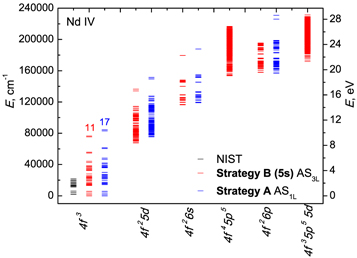
Figure 4. Energy levels for configurations of Nd ii compared with NIST data. Black represents NIST data, red represents our computed energy levels in Strategy B (5s)  , and blue data are based on Strategy A
  . The numbers above the red and blue columns are averaged disagreements in percent for the levels of each configuration, compared with the NIST database.
Download figure:
Standard image High-resolution imageTable 6. Comparison of Energy Levels in the NIST Database (in %) of Nd iv by Increase of the Active Space Performed, Applying Strategies A, B, and B with 5s
| Strategy A | Strategy B | Strategy B (5s) | ||||
|---|---|---|---|---|---|---|
| Config. | Term | J | NIST |

|

|

|

|

|
9/2 | 0 | |||
| 11/2 | [1880] | 6.8/6.5/6.4 | 6.9/6.8/6.7 | 7.2/7.1/7.0 | ||
| 13/2 | [3860] | 5.6/5.4/5.3 | 5.8/5.8/5.7 | 6.1/6.1/6.0 | ||
| 15/2 | [5910] | 4.7/4.6/4.6 | 4.9/5.0/5.0 | 5.2/5.3/5.3 | ||

|

|
3/2 | [11290] | −27.8/−27.0/−26.6 | −20.3/−19.2/−18.6 | −17.6/−16.4/−15.8 |
| 5/2 | [12320] | −24.8/−24.2/−23.8 | −17.9/−16.9/−16.4 | −15.3/−14.4/−13.8 | ||

|

|
9/2 | [12470] | −14.7/−12.5/−11.3 | −12.8/−10.4/−9.4 | −12.0/−9.5/−8.5 |

|

|
7/2 | [13280] | −22.3/−21.6/−21.2 | −16.1/−15.2/−14.6 | −13.7/−12.8/−12.3 |

|

|
3/2 | [13370] | −20.2/−16.8/−16.5 | −15.6/−12.1/−11.6 | −13.3/−9.8/−9.3 |

|

|
9/2 | [14570] | −18.3/−17.6/−17.1 | −13.2/−12.1/−11.6 | −11.3/−10.2/−9.7 |

|

|
11/2 | [15800] | −9.6/−7.8/−6.8 | −8.4/−6.3/−5.5 | −7.8/−5.7/−4.9 |

|

|
5/2 | [16980] | −29.6/−28.1/−27.8 | −21.7/−20.2/−19.6 | −18.6/−17.1/−16.5 |

|

|
7/2 | [17100] | |||

|

|
7/2 | [18890] | −23.6/−22.3/−22.0 | −16.9/−15.5/−14.9 | −14.3/−12.9/−12.3 |
| 9/2 | [19290] | −16.6/−27.0/−26.7 | −22.1/−20.6/−20.0 | −19.7/−18.3/−17.7 | ||

|

|
13/2 | [19440] | −17.7/−15.0/−14.2 | −15.1/−12.2/−11.4 | −13.9/−11.1/−10.3 |

|

|
11/2 | [21280] | −22.2/−21.0/−20.8 | −15.9/−14.6/−14.2 | −13.4/−12.2/−11.7 |

|

|
15/2 | [21430] | −16.1/−13.7/−12.9 | −13.6/−11.0/−10.3 | −12.5/−9.9/−9.2 |
Note. States marked with the subscript * in the term column are without a term identification in the NIST database.
Download table as: ASCIITypeset image
For the Nd iv ion, several experiments and analyses with semi-empirical methods have been performed. The emission spectrum produced by vacuum spark sources was observed in the vacuum ultraviolet on two normal-incidence spectrographs. 550 lines have been identified as transitions from 85 (out of 107 possible) levels of  to 37 (out of 41 possible) levels of
  . The method and codes of Cowan were used to predict the spectral ranges of the strong transitions in the spectra Nd iv at the beginning of the series of paper (Wyart et al. 2006).
Later, Wyart et al. (2007) used the same experiment to observe and classify 1426 lines. In total, 41 levels of  configuration were reported. To derive energy levels with the diagonalization code RCG, the input Hartree–Fock radial integrals including relativistic corrections, treated as parameters (HFR parameters), were scaled according to earlier results on the neighboring ion spectra. Altogether 111 odd parity and 121 even parity configuration levels for
  ,
,  ,
,  ,
,  ,
,  , and
, and  were established. Their optimized values were calculated with the ELCALC code (Radziemski et al. 1970).
Then, Wyart et al. (2008) performed a parametric fit of the level energies for the  configuration, previously obtained in the experiment (Wyart et al. 2007). Dzuba et al. (2003) used the same computations applied to Nd iii (see Section 4.2). This included only 72 levels of configurations
  and
and  . In Table 7, the energy levels obtained from applying Strategy B with 5s are compared with the experimental values from Wyart et al. (2007) and semi-empirical values from Dzuba et al. (2003).
Table 7. Comparison of Energy Levels from Present (Strategy B with 5s) and Other Theoretical Computations with the NIST Database (in %) and with the Experimental Wyart et al. (2007; in %) Values of Nd iv
| Present | Dzuba et al. (2003) | ||||||
|---|---|---|---|---|---|---|---|
| Config. | Term | J | NIST | Exp. |

|
Cowan | RCI |

|

|
9/2 | 0 | 0 | 0 | 0 | 0 |
| 11/2 | [1880] | 1897.11 | 1749/7.0/7.8 | 1879/0.1/1.0 | 1945/−3.5/−2.5 | ||
| 13/2 | [3860] | 3907.43 | 3627/6.0/7.2 | 3890/−0.8/0.4 | 4049/−4.9/−3.6 | ||
| 15/2 | [5910] | 5988.51 | 5596/5.3/6.6 | 5989/−1.3/0.0 | 6267/−6.0/−4.7 | ||

|

|
3/2 | [11290] | 11698.49 | 13076/−15.8/−11.8 | 13294/−17.8/−13.6 | 12490/−10.6/−6.8 |
| 5/2 | [12320] | 12747.94 | 14022/−13.8/−10.0 | 14333/−16.3/−12.4 | 13545/−9.9/−6.3 | ||

|

|
9/2 | [12470] | 12800.29 | 13536/−8.5/−5.8 | 13272/−6.4/−3.7 | 14522/−16.5/−13.5 |

|

|
7/2 | [13280] | 13719.82 | 14911/−12.3/−8.7 | 15249/−14.8/−11.1 | 14622/−10.1/−6.6 |

|

|
3/2 | [13370] | 13792.49 | 14617/−9.3/−6.0 | 15153/−13.3/−9.9 | 14452/−8.1/−4.8 |

|

|
9/2 | [14570] | 14994.87 | 15979/−9.7/−6.6 | 16334/−12.1/−8.9 | 16183/−11.1/−7.9 |

|

|
11/2 | [15800] | 16161.53 | 16581/−4.9/−2.6 | 16456/−4.2/−1.8 | 18142/−14.8/−12.3 |

|

|
5/2 | [16980] | 17707.17 | 19780/−16.5/−11.7 | ||

|

|
7/2 | [17100] | 17655.11 | |||

|

|
7/2 | [18890] | 19540.80 | 21218/−12.3/−8.6 | ||
| 9/2 | [19290] | 19969.79 | 22709/−17.7/−13.7 | ||||

|

|
13/2 | [19440] | 20005.22 | 21445/−10.3/−7.2 | ||

|

|
11/2 | [21280] | 22047.39 | 23768/−11.7/−7.8 | ||

|

|
15/2 | [21430] | 22043.77 | 23398/−9.2/−6.1 | ||
Note. States marked by the subscript * in the term column are without term identification in the NIST database.
Download table as: ASCIITypeset image
In addition to the energy levels, transition data can also be compared with experimental data and semi-empirical calculations (Table 8). Our results for the transition wavelengths show good agreement with the experimental data by Wyart et al. (2007). As shown in Figure 5, the agreement in the wavelength is within 20% for most transitions.
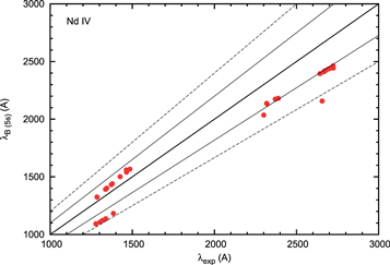
Figure 5. Comparison of transition wavelengths for Nd iv between our results from Strategy B with 5s and experimental data by Wyart et al. (2007). The thick line corresponds to perfect agreement, while thin solid and dashed lines correspond to 10% and 20% deviations.
Download figure:
Standard image High-resolution imageTable 8.
Computed Transition Data of Nd iv from Applying Strategy B with 5s at  , Compared with the Experimental Wavelength
  (in Å) and Computed Transition Probabilities ASE (in s−1) from Wyart et al. (2007)
| Strategies B with 5s | Wyart et al. (2007) | Yoca & Quinet (2014) | ||||||||
|---|---|---|---|---|---|---|---|---|---|---|
| Upper | Lower |

|

|
dT | λ | ASE |

|
ASE | ||

|
4.5 |

|
4.5 | 5.26E+8 | 4.40E+8 | 0.16 | 1107.72(15.0) | 4.04E+8 | 1303.32 | 3.89E+8 |

|
7.5 |

|
8.5 | 9.32E+7 | 1.24E+8 | 0.25 | 1540.16(−5.1) | 1.64E+8 | 1464.73 | 1.47E+8 |

|
5.5 |

|
5.5 | 2.04E+8 | 1.91E+8 | 0.06 | 2412.27(9.5) | 1.96E+8 | 2666.70 | 1.94E+8 |

|
4.5 |

|
3.5 | 1.92E+8 | 1.61E+8 | 0.16 | 2410.31(9.6) | 1.97E+8 | 2666.70 | 1.96E+8 |

|
6.5 |

|
7.5 | 6.85E+7 | 8.99E+7 | 0.24 | 1559.66(−6.6) | 1.28E+8 | 1463.34 | 1.14E+8 |

|
5.5 |

|
6.5 | 3.78E+7 | 5.67E+7 | 0.33 | 1324.01(−3.0) | 8.92E+7 | 1285.61 | 6.48E+7 |

|
4.5 |

|
5.5 | 4.11E+7 | 6.19E+7 | 0.34 | 1325.17(−3.1) | 1.04E+8 | 1285.38 | 7.55E+7 |

|
3.5 |

|
4.5 | 7.27E+7 | 1.03E+8 | 0.29 | 1401.4 (−4.2) | 1.29E+8 | 1344.74 | 1.17E+8 |

|
4.5 |

|
5.5 | 1.01E+9 | 8.05E+8 | 0.20 | 1123.17(14.9) | 7.61E+8 | 1319.25 | 7.29E+8 |

|
5.5 |

|
6.5 | 1.55E+8 | 1.65E+8 | 0.06 | 2157.57(18.8) | 2.17E+8 | 2656.02 | 2.16E+8 |

|
5.5 |

|
5.5 | 2.30E+8 | 2.17E+8 | 0.06 | 2443.54(10.3) | 1.70E+8 | 2723.51 | 1.86E+8 |

|
4.5 |

|
5.5 | 2.02E+8 | 2.07E+8 | 0.02 | 2416.08(9.5) | 2.00E+8 | 2670.03 | 2.04E+8 |

|
3.5 |

|
4.5 | 1.95E+8 | 2.00E+8 | 0.02 | 2423.25(9.5) | 1.99E+8 | 2678.00 | |

|
5.5 |

|
6.5 | 7.27E+7 | 1.04E+8 | 0.30 | 1391.9 (−4.1) | 1.29E+8 | 1336.98 | 1.00E+8 |

|
7.5 |

|
7.5 | 4.69E+7 | 8.18E+7 | 0.43 | 1432.37(−4.4) | 9.05E+7 | 1372.20 | 7.44E+7 |

|
5.5 |

|
6.5 | 1.16E+8 | 1.20E+8 | 0.03 | 2443.59(10.3) | 1.17E+8 | 2723.51 | 1.22E+8 |

|
4.5 |

|
4.5 | 1.38E+8 | 1.30E+8 | 0.05 | 2436.05(9.6) | 1.27E+8 | 2694.71 | |

|
4.5 |

|
5.5 | 7.02E+7 | 9.97E+7 | 0.30 | 1397.63(−4.1) | 1.24E+8 | 1342.01 | 1.10E+8 |

|
6.5 |

|
5.5 | 3.29E+8 | 2.88E+8 | 0.13 | 2174 (8.3) | 2.84E+8 | 2370.51 | 2.94E+8 |

|
3.5 |

|
4.5 | 2.86E+8 | 2.88E+8 | 0.01 | 2394.67(9.4) | 2.89E+8 | 2643.03 | 2.93E+8 |

|
6.5 |

|
6.5 | 7.68E+7 | 7.75E+7 | 0.01 | 2181.33(8.7) | 8.11E+7 | 2388.79 | 1.26E+8 |

|
7.5 |

|
8.5 | 1.34E+9 | 1.07E+9 | 0.20 | 1093.02(14.5) | 6.16E+8 | 1278.41 | 6.63E+8 |

|
6.5 |

|
7.5 | 7.92E+8 | 6.02E+8 | 0.24 | 1182.67(14.6) | 4.37E+8 | 1385.21 | 4.89E+8 |

|
6.5 |

|
5.5 | 4.95E+8 | 4.43E+8 | 0.10 | 2132.31(8.1) | 3.65E+8 | 2320.43 | 4.09E+8 |

|
5.5 |

|
4.5 | 5.00E+8 | 4.56E+8 | 0.09 | 2137.32(7.8) | 4.15E+8 | 2318.07 | 3.98E+8 |

|
5.5 |

|
4.5 | 1.90E+7 | 1.56E+7 | 0.18 | 2035.66(11.5) | 3.96E+8 | 2300.68 | 4.16E+8 |

|
5.5 |

|
5.5 | 2.85E+8 | 2.39E+8 | 0.16 | 1136.61(15.1) | 1.54E+8 | 1338.62 | 1.03E+8 |

|
6.5 |

|
7.5 | 6.41E+7 | 8.42E+7 | 0.24 | 1501.86(−5.3) | 1.27E+8 | 1426.05 | 1.14E+8 |

|
4.5 |

|
4.5 | 1.78E+8 | 1.65E+8 | 0.07 | 2443.44(9.8) | 1.71E+8 | 2708.43 | 1.70E+8 |

|
5.5 |

|
5.5 | 1.16E+8 | 1.10E+8 | 0.06 | 2462.26(9.6) | 1.18E+8 | 2723.34 | 1.23E+8 |

|
6.5 |

|
6.5 | 4.40E+7 | 7.69E+7 | 0.43 | 1440.32(−4.5) | 8.54E+7 | 1378.09 | 6.95E+7 |

|
6.5 |

|
7.5 | 3.75E+7 | 4.99E+7 | 0.25 | 1566.59(−5.4) | 7.14E+7 | 1485.64 | 6.43E+7 |
Download table as: ASCIITypeset image
Table 9. Energy Levels (in cm−1) Relative to the Ground State for the Lowest States of Nd ii
| No. | label | J | P | E |
|---|---|---|---|---|
| 1 |

|
7/2 | + | 0.00 |
| 2 |

|
9/2 | + | 547.86 |
| 3 |

|
11/2 | + | 1404.36 |
| 4 |

|
9/2 | + | 1789.52 |
| 5 |

|
13/2 | + | 2425.58 |
| 6 |

|
11/2 | + | 3120.96 |
| 7 |

|
15/2 | + | 3564.21 |
| 8 |

|
11/2 | + | 4019.24 |
| 9 |

|
13/2 | + | 4506.07 |
| 10 |

|
17/2 | + | 4789.43 |
| 11 |

|
13/2 | + | 4941.03 |
| 12 |
|
13/2 | − | 5477.69 |
| 13 |

|
15/2 | + | 5940.53 |
| 14 |

|
15/2 | + | 5965.42 |
| 15 |

|
9/2 | + | 6065.11 |
| 16 |

|
15/2 | − | 6750.71 |
| 17 |

|
11/2 | + | 6881.31 |
| 18 |

|
17/2 | + | 7078.84 |
| 19 |

|
13/2 | + | 7802.57 |
| 20 |

|
17/2 | − | 8147.61 |
Note. Table 9 is published in its entirety in machine-readable format. A portion of the table is shown here for guidance regarding its form and content.
Only a portion of this table is shown here to demonstrate its form and content. A machine-readable version of the full table is available.
Download table as: DataTypeset image
Table 10.
Transition Energies  (in cm−1), Transition Wavelengths λ (in Å), Line Strengths S (in a.u.), Weighted Oscillator Strengths gf, and Transition Rates A (in s−1) for E1 Transitions of the Nd ii ion
| upper | lower |

|
λ | S | gf | A | dT |
|---|---|---|---|---|---|---|---|

|

|
22745 | 4396.48 | 4.593E+00 | 3.173E−01 | 9.127E+06 | 0.050 |

|
|
23391 | 4275.02 | 1.001E+01 | 7.115E−01 | 2.164E+07 | 0.154 |

|
|
24959 | 4006.51 | 7.628E−01 | 5.783E−02 | 2.002E+06 | 0.130 |

|
|
25373 | 3941.14 | 1.380E+00 | 1.063E−01 | 3.807E+06 | 0.033 |

|
|
26882 | 3719.95 | 2.049E−01 | 1.673E−02 | 6.722E+05 | 0.041 |

|
|
27650 | 3616.62 | 1.213E−01 | 1.018E−02 | 4.330E+05 | 0.069 |

|

|
28842 | 3467.14 | 5.807E−02 | 5.088E−03 | 2.352E+05 | 0.351 |

|

|
29386 | 3402.93 | 3.867E−01 | 3.452E−02 | 1.657E+06 | 0.120 |

|
|
29450 | 3395.57 | 1.159E−02 | 1.037E−03 | 5.002E+04 | 0.124 |

|
|
30233 | 3307.58 | 5.567E−02 | 5.112E−03 | 2.597E+05 | 0.164 |

|
|
30410 | 3288.31 | 3.589E−02 | 3.316E−03 | 1.704E+05 | 0.320 |

|

|
30982 | 3227.58 | 2.441E−04 | 2.297E−05 | 1.226E+03 | 0.999 |

|

|
31155 | 3209.69 | 5.477E−02 | 5.184E−03 | 2.797E+05 | 0.186 |

|

|
31541 | 3170.46 | 3.420E−02 | 3.276E−03 | 1.812E+05 | 0.373 |

|
|
31848 | 3139.89 | 2.205E−04 | 2.133E−05 | 1.202E+03 | 0.541 |

|
|
32432 | 3083.34 | 5.245E−03 | 5.167E−04 | 3.021E+04 | 0.319 |

|
|
33244 | 3008.02 | 2.221E−03 | 2.242E−04 | 1.377E+04 | 0.427 |

|
|
33332 | 3000.04 | 1.985E−05 | 2.010E−06 | 1.241E+02 | 0.938 |

|
|
33384 | 2995.44 | 1.588E−04 | 1.611E−05 | 9.980E+02 | 0.446 |
|
|
33499 | 2985.08 | 8.480E−04 | 8.629E−05 | 5.383E+03 | 0.424 |
Note. All transition data are in length form. dT is the relative difference of the transition rates in length and velocity form as given by Equation (5). Table 10 is published in its entirety in machine-readable format. A portion of the table is shown here for guidance regarding its form and content.
Only a portion of this table is shown here to demonstrate its form and content. A machine-readable version of the full table is available.
Download table as: DataTypeset image
We also confirmed a nice agreement in the transition probabilities. Table 8 and Figure 6 show transition probabilities for the strongest transitions computed by Wyart et al. (2007). Our results and theirs agree within a factor of 2. Note that semi-empirical calculations have uncertainties. Using the same HFR method combined with parametric least-squares fits to the same experimental data with Wyart et al. (2007), Yoca & Quinet (2014) computed and presented transition probabilities (only with  ), oscillator strengths, and radiative lifetimes in bigger multiconfiguration expansions than Wyart et al. (2007). Their results are systematically different, and those by Yoca & Quinet (2014) in fact show a slightly better agreement with ours, as shown in the bottom panel of Figure 6.
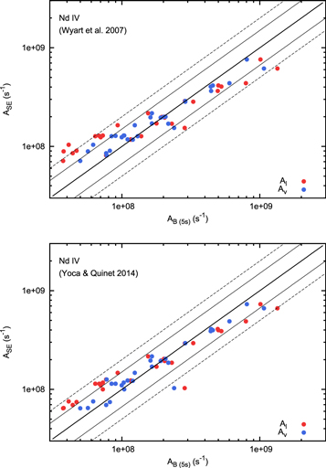
Figure 6. Comparison of transition probability for Nd iv. The top and bottom panels show a comparison between our results from Strategy B with 5s and semi-empirical results by Wyart et al. (2007) and by Yoca & Quinet (2014), respectively. The thick line corresponds to perfect agreement, while the thin solid and dashed lines correspond to deviations by factors of 1.5 and 2.0, respectively. The red and blue points show the values calculated with the length (Babushkin) and velocity (Coulomb) forms, respectively.
Download figure:
Standard image High-resolution imageTable 11. Energy Levels (in cm−1) Relative to the Ground State for the Lowest States of Nd iii
| No. | label | J | P | E |
|---|---|---|---|---|
| 1 |

|
4 | + | 0.00 |
| 2 |

|
5 | + | 1072.58 |
| 3 |

|
6 | + | 2263.93 |
| 4 |

|
7 | + | 3542.92 |
| 5 |

|
8 | + | 4884.66 |
| 6 |

|
1 | + | 11739.04 |
| 7 |

|
2 | + | 12098.57 |
| 8 |

|
3 | + | 12724.33 |
| 9 |

|
2 | + | 13433.63 |
| 10 |

|
4 | + | 13459.96 |
| 11 |

|
5 | + | 14444.26 |
| 12 |

|
6 | + | 15065.97 |
| 13 |

|
5 | − | 15128.43 |
| 14 |

|
6 | − | 15257.69 |
| 15 |

|
4 | + | 16151.40 |
| 16 |

|
7 | + | 16180.31 |
| 17 |

|
6 | − | 16720.95 |
| 18 |

|
7 | − | 16985.08 |
| 19 |

|
2 | + | 17295.05 |
| 20 |

|
3 | + | 17368.09 |
Note. Table 11 is published in its entirety in machine-readable format. A portion of the table is shown here for guidance regarding its form and content.
Only a portion of this table is shown here to demonstrate its form and content. A machine-readable version of the full table is available.
Download table as: DataTypeset image
Table 12.
Transition Energies  (in cm−1), Transition Wavelengths λ (in Å), Line Strengths S (in a.u.), Weighted Oscillator Strengths gf, and Transition Rates A (in s−1) for E1 Transitions of the Nd iii Ion
| upper | lower |

|
λ | S | gf | A | dT |
|---|---|---|---|---|---|---|---|

|

|
6521 | 15334.41 | 2.338E−03 | 4.632E−05 | 4.380E+02 | 0.948 |

|

|
9156 | 10920.99 | 1.996E−02 | 5.553E−04 | 1.035E+04 | 0.861 |

|

|
10206 | 9798.04 | 5.262E−03 | 1.631E−04 | 3.778E+03 | 0.787 |

|

|
10697 | 9348.19 | 8.930E−03 | 2.901E−04 | 7.382E+03 | 0.822 |

|

|
11516 | 8683.29 | 3.115E−05 | 1.090E−06 | 3.214E+01 | 0.890 |

|

|
12113 | 8255.57 | 1.272E−02 | 4.681E−04 | 1.527E+04 | 0.752 |

|

|
14250 | 7017.52 | 9.589E−02 | 4.150E−03 | 1.874E+05 | 0.710 |

|

|
17425 | 5738.84 | 7.686E−02 | 4.068E−03 | 2.746E+05 | 0.647 |

|

|
18400 | 5434.62 | 5.429E−04 | 3.034E−05 | 2.284E+03 | 0.634 |

|

|
19753 | 5062.36 | 1.351E−02 | 8.110E−04 | 7.036E+04 | 0.786 |

|

|
20499 | 4878.06 | 4.216E−03 | 2.625E−04 | 2.453E+04 | 0.562 |

|

|
20588 | 4857.14 | 6.608E−02 | 4.132E−03 | 3.894E+05 | 0.679 |

|

|
21850 | 4576.58 | 4.184E−02 | 2.777E−03 | 2.948E+05 | 0.711 |

|

|
22166 | 4511.37 | 1.708E−05 | 1.150E−06 | 1.257E+02 | 0.812 |

|

|
22582 | 4428.21 | 7.961E−03 | 5.461E−04 | 6.192E+04 | 0.707 |

|

|
23964 | 4172.76 | 1.943E−02 | 1.415E−03 | 1.806E+05 | 0.137 |

|

|
24808 | 4030.93 | 4.263E−04 | 3.213E−05 | 4.396E+03 | 0.318 |

|

|
25324 | 3948.70 | 3.464E−03 | 2.665E−04 | 3.800E+04 | 0.784 |

|

|
26223 | 3813.37 | 2.834E−03 | 2.257E−04 | 3.452E+04 | 0.389 |

|

|
27992 | 3572.45 | 4.279E−09 | 3.638E−10 | 6.339E-02 | 0.999 |
Note. All transition data are in length form. dT is the relative difference of the transition rates in length and velocity form as given by Equation (5). Table 12 is published in its entirety in machine-readable format. A portion of the table is shown here for guidance regarding its form and content.
Only a portion of this table is shown here to demonstrate its form and content. A machine-readable version of the full table is available.
Download table as: DataTypeset image
5. Impact on the Opacities
We calculate bound-bound opacities using our results to study the impact of the accuracy on the atomic calculations. By following previous works on NS mergers (Barnes & Kasen 2013; Kasen et al. 2013; Tanaka & Hotokezaka 2013; Tanaka et al. 2014, 2018), we use the formalism of expansion opacity (Karp et al. 1977; Eastman & Pinto 1993; Kasen et al. 2006):

Here, ρ and t represent density and time after the merger. The summation is taken over all the transitions in a wavelength bin ( ), and
  and
and  are the transition wavelength and the Sobolev optical depth for each transition. The Sobolev optical depth
  is expressed as

where gl, El, and fl are the statistical weight and the energy of the lower level of the transition and the oscillator strength of the transition, respectively. For the oscillator strength, we use results computed with the length (Babushkin) form. For the number density at the lower level of the transition (nl), the Boltzmann distribution is assumed, i.e.,  , where g0 is the statistical weight for the ground level. The number density of each ion n is calculated under the assumption of local thermodynamic equilibrium using the Saha equation. In this paper, pure Nd gas is assumed. We use all the calculated transitions to evaluate the opacity without any selection based on the transition strengths, which was applied in full radiative transfer simulations (Tanaka et al. 2017).
Table 13. Energy Levels (in cm−1) Relative to the Ground State for the Lowest States of Nd iV
| No. | label | J | P | E |
|---|---|---|---|---|
| 1 |

|
9/2 | − | 0.00 |
| 2 |

|
11/2 | − | 1748.59 |
| 3 |

|
13/2 | − | 3627.05 |
| 4 |

|
15/2 | − | 5595.78 |
| 5 |

|
3/2 | − | 13076.19 |
| 6 |

|
9/2 | − | 13536.44 |
| 7 |

|
5/2 | − | 14022.10 |
| 8 |

|
3/2 | − | 14617.16 |
| 9 |

|
7/2 | − | 14911.07 |
| 10 |

|
9/2 | − | 15979.23 |
| 11 |

|
11/2 | − | 16581.13 |
| 12 |

|
7/2 | − | 18780.28 |
| 13 |

|
5/2 | − | 19780.48 |
| 14 |

|
9/2 | − | 21211.00 |
| 15 |

|
7/2 | − | 21217.90 |
| 16 |

|
13/2 | − | 21444.78 |
| 17 |

|
9/2 | − | 22708.88 |
| 18 |

|
3/2 | − | 23160.03 |
| 19 |

|
15/2 | − | 23397.52 |
| 20 |

|
11/2 | − | 23768.32 |
Note. Table 13 is published in its entirety in machine-readable format. A portion of the table is shown here for guidance regarding its form and content.
Only a portion of this table is shown here to demonstrate its form and content. A machine-readable version of the full table is available.
Download table as: DataTypeset image
Table 14.
Transition Energies  (in cm−1), Transition Wavelengths λ (in Å), Line Strengths S (in a.u.), Weighted Oscillator Strengths gf, and Transition Rates A (in s−1) for E1 Transitions of the Nd iv ion
| upper | lower |

|
λ | S | gf | A | dT |
|---|---|---|---|---|---|---|---|

|

|
52003 | 1922.95 | 3.607E−02 | 5.698E−03 | 5.140E+06 | 0.422 |

|

|
44283 | 2258.20 | 7.141E−03 | 9.606E−04 | 6.283E+05 | 0.235 |

|

|
83619 | 1195.89 | 3.829E−07 | 9.725E−08 | 2.268E+02 | 0.945 |

|

|
85201 | 1173.69 | 2.099E−05 | 5.432E−06 | 1.315E+04 | 0.116 |

|
|
92307 | 1083.33 | 1.546E−05 | 4.336E−06 | 1.232E+04 | 0.249 |

|

|
96617 | 1035.01 | 2.052E−05 | 6.022E−06 | 1.875E+04 | 0.739 |

|

|
99613 | 1003.88 | 9.090E−05 | 2.750E−05 | 9.102E+04 | 0.448 |

|

|
103718 | 964.15 | 2.294E−06 | 7.228E−07 | 2.593E+03 | 0.625 |

|

|
105216 | 950.42 | 5.732E−04 | 1.832E−04 | 6.764E+05 | 0.229 |

|
|
108119 | 924.90 | 1.258E−02 | 4.132E−03 | 1.611E+07 | 0.069 |

|

|
109048 | 917.03 | 6.412E−04 | 2.124E−04 | 8.424E+05 | 0.310 |

|
|
109666 | 911.85 | 4.762E−06 | 1.586E−06 | 6.363E+03 | 0.182 |

|
|
110081 | 908.41 | 5.629E−05 | 1.882E−05 | 7.608E+04 | 0.611 |

|

|
110468 | 905.24 | 1.101E−03 | 3.695E−04 | 1.503E+06 | 0.170 |
|

|
112421 | 889.51 | 1.612E−03 | 5.508E−04 | 2.321E+06 | 0.089 |

|

|
113266 | 882.87 | 1.875E−04 | 6.451E−05 | 2.760E+05 | 0.153 |

|
|
115617 | 864.92 | 3.828E−03 | 1.344E−03 | 5.994E+06 | 0.192 |

|

|
116976 | 854.87 | 6.502E−05 | 2.310E−05 | 1.054E+05 | 0.454 |

|
|
118179 | 846.17 | 3.156E−03 | 1.133E−03 | 5.277E+06 | 0.251 |

|

|
119038 | 840.07 | 5.618E−03 | 2.031E−03 | 9.600E+06 | 0.113 |
Note. All transition data are in length form. dT is the relative difference of the transition rates in length and velocity form as given by equation (5). Table 14 is published in its entirety in machine-readable format. A portion of the table is shown here for guidance regarding its form and content.
Only a portion of this table is shown here to demonstrate its form and content. A machine-readable version of the full table is available.
Download table as: DataTypeset image
We find that the overall properties of opacities are not dramatically affected by the accuracies of the atomic calculations. The left panels in Figure 7 show the expansion opacities calculated by using transition data of Nd ii, Nd iii, and Nd iv. The temperatures are assumed to be 5000 K, 10,000 K, and 15,000 K for Nd ii, Nd iii, and Nd iv, respectively. The density is  and the time after the merger is set to 1 day. The overall opacity values and wavelength dependencies are quite similar for different atomic calculations. The red lines show the best results in this paper, while the blue lines show the previous results used by Tanaka et al. (2018).

Figure 7. Opacities for the Nd ii (top), Nd iii (middle), and Nd iv (bottom) ions. The left panels show the expansion opacities calculated with T = 5000 K, 10,000 K, and 15,000 K for Nd ii, Nd iii, and Nd iv, respectively. The density and time are assumed to be  and t = 1 day after the merger, respectively. The right panels show the Planck mean opacities for various temperatures. The dashed curve shows the Planck mean opacities calculated with atomic data for Nd i-iv calculated with the HULLAC code (Tanaka et al. 2018).
Download figure:
Standard image High-resolution imageThe behavior of the opacity is similar for different temperatures. The right panels show the Planck mean opacities calculated for different temperatures by keeping the density and time to as the same. The Planck mean opacities from different atomic calculations agree with each other within a factor of 1.5. Since the timescale of the kilonova emission scales as  (Rosswog 2015; Fernández & Metzger 2016; Tanaka 2016; Metzger 2017), this level of difference does not significantly affect the timescale of kilonovae (smaller than ∼20%) compared with those expected from differences in temperature and abundances.
Taking a closer look, however, the wavelength-dependent opacities show some differences. The most notable difference is the feature around 4000 Å in the case of Nd ii. The new GRASP2K calculations with better accuracy show a bump, while the old GRASP2K calculations and HULLAC calculations do not, creating a difference in the opacity by a factor of 2. Interestingly, Kasen et al. (2013) also showed that this part of the opacity is affected by the optimization in the atomic calculations: the peak is located near 5000 Å in their opt1 case, while the peak is weaker in their opt2 and opt3 cases. The expansion opacities presented by Fontes et al. (2017) also show a peak around 4000 Å, which is close to our new results.
We find that the difference between our new and previous opacities is caused by the lower energy levels of  and
and  configurations in our new calculations (Figure 1). Figure 8 shows the number of strong transitions that fulfill
  at T = 5000 K. The numbers of transitions are separated according to the lower level configuration. The numbers of strong transitions from the levels of the
  and
and  configuration is enhanced around 4500 Å in our new calculations (Strategy C
  ). Since the energies of these configurations were overestimated in our previous calculations (Strategy A
  , Figure 1), the bump structure in the new calculations seems more realistic. This demonstrates the importance of accurate calculations for lower energy levels to predict the spectra of kilonovae.
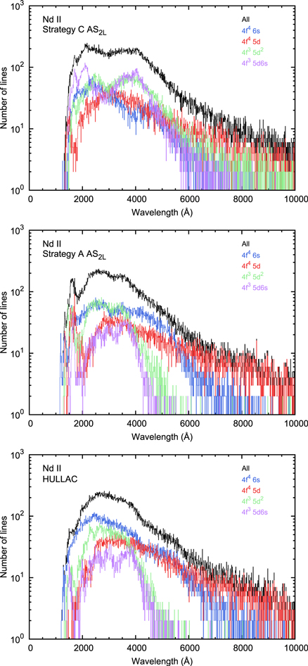
Figure 8. Number of strong transitions of Nd ii as a function of wavelength. The strong transitions are selected by the criterion  with T = 5000 K. The black lines show the total number of strong transitions and the color lines show transitions from each lower-level configuration.
Download figure:
Standard image High-resolution imageFigure 9 shows the cumulative number of states (CNS) for  and
and  configurations as a function of excitation energies. Note that the number of states takes the statistical weight (degeneracy) of each level, i.e.
  , into account. The CNS for all the energy levels obtained by GRASP2K and HULLAC calculations is compared in the figure. The CNS of the new calculations rises at lower energy and has larger values than those of the previous calculations with GRASP2K and HULLAC, indicating that the larger number of states falls into the lower-energy region with the new calculations. Since the Boltzmann distribution is assumed for the number density in the lower levels of transitions, it is predicted that the number of strong transitions from the levels of
  and
and  configurations becomes larger with the new calculations, as depicted in Figure 8. This is more remarkable for the
  configuration as in the CNS. The CNS of the new calculations is also compared with those of NIST and the semi-empirical results by Wyart (2010). The overall agreement is good at low energies, convincing us of the accuracy of our new calculations. The only exception is the semi-empirical results for the
  configuration, which overshoot significantly at high energies. The source of this discrepancy is yet to be investigated.

Figure 9. Cumulative number of states for  (a,b) and
  (c,d) configurations as a function of excitation energy. (a,c): results with the present and previous GRASP2K and HULLAC calculations. (b,d): results with the present GRASP2K calculation, NIST, and the semi-empirical method by Wyart (2010).
Download figure:
Standard image High-resolution image
Another notable difference is a feature around 1000 Å: the opacities in our new calculations are suppressed. This is due to the inclusion of highly excited energy levels in the previous calculations (both GRASP2K and HULLAC). Therefore, the opacities in the ultraviolet wavelengths depend on the choice of the configurations included in the calculations. However, if configurations with sufficiently high energy ( ) are included, this difference appears only in the far-ultraviolet wavelength, and thus does not affect observable features.
6. Summary
We presented extensive atomic calculations of neodymium and studied the impact of accuracies in the calculations on the astrophysical opacities. The extended search for electron correlation effect inclusion strategies is presented in this work for the three Nd ions (Nd II-IV). In total, 6000, 1453, and 1533 levels are presented for Nd ii, Nd iii, and Nd iv respectively, and E1 type transitions between these levels were computed. Exclusive accuracy is achieved for atomic energy spectra results. Compared with the NIST database, the averaged relative differences are 10%, 3%, and 11% for Nd ii, Nd iii, and Nd iv, respectively.
Using our new results, we calculated the expansion opacities used in radiative transfer simulations for kilonovae, radioactively powered EM emission from NS mergers. We found that the overall opacity values and their wavelength dependence are not very sensitive to the accuracies of the calculations. The Planck mean opacities from our previous and new atomic calculations agree within a factor of 1.5. This confirms the validity of previous studies of kilonovae.
However, some wavelength-dependent features are affected by the accuracy of the atomic calculations. In particular, the low-lying energy levels ( eV) can affect the opacities and even produce a bump in certain wavelength ranges. Our results highlight the importance of accurate atomic calculations for low-lying energy levels to accurately predict the spectra of kilonovae.
This research was funded by a grant (No. S-LJB-18-1) from the Research Council of Lithuania. This research was also supported by the JSPS Bilateral Joint Research Project. The computations presented in this paper were performed at the High Performance Computing Center "HPC Sauletekis" of the Faculty of Physics at Vilnius University and with Cray XC30 and XC50 at the Center for Computational Astrophysics, National Astronomical Observatory of Japan. D.K. is grateful for the support by the NINS program of Promoting Research by Networking among Institutions (grant No. 01411702). M.T. is supported by the NINS program for cross-disciplinary science study, Inoue Science Research Award from Inoue Foundation for Science, and the Grant-in-Aid for Scientific Research from JSPS (15H02075, 16H02183) and MEXT (17H06363).