


Abstract
We present high-precision timing data over time spans of up to 11 years for 45 millisecond pulsars observed as part of the North American Nanohertz Observatory for Gravitational Waves (NANOGrav) project, aimed at detecting and characterizing low-frequency gravitational waves. The pulsars were observed with the Arecibo Observatory and/or the Green Bank Telescope at frequencies ranging from 327 MHz to 2.3 GHz. Most pulsars were observed with approximately monthly cadence, and six high-timing-precision pulsars were observed weekly. All were observed at widely separated frequencies at each observing epoch in order to fit for time-variable dispersion delays. We describe our methods for data processing, time-of-arrival (TOA) calculation, and the implementation of a new, automated method for removing outlier TOAs. We fit a timing model for each pulsar that includes spin, astrometric, and (for binary pulsars) orbital parameters; time-variable dispersion delays; and parameters that quantify pulse-profile evolution with frequency. The timing solutions provide three new parallax measurements, two new Shapiro delay measurements, and two new measurements of significant orbital-period variations. We fit models that characterize sources of noise for each pulsar. We find that 11 pulsars show significant red noise, with generally smaller spectral indices than typically measured for non-recycled pulsars, possibly suggesting a different origin. A companion paper uses these data to constrain the strength of the gravitational-wave background.
Export citation and abstract BibTeX RIS
1. Introduction
High-precision timing of millisecond pulsars offers the promise of detecting gravitational waves with periods of a few years, i.e., in the nanohertz (nHz) band of the gravitational-wave spectrum (Burke-Spolaor 2015; Lommen 2015). An expected signal in this band is the incoherent superposition of gravitational waves from the cosmic merger history of supermassive black hole binaries, i.e., a gravitational-wave background (Phinney 2001; Jaffe & Backer 2003; Sesana 2013). Its detection is likely within a few years (Taylor et al. 2016), depending on the underlying astrophysics of supermassive black hole binary mergers (Kocsis & Sesana 2011; Roedig et al. 2012; Sampson et al. 2015; Arzoumanian et al. 2016; Taylor et al. 2017). Other possible sources of gravitational waves in this band are individual massive binary systems (Arzoumanian et al. 2014; Babak et al. 2016), gravitational bursts with memory (e.g., Seto 2009; Madison et al. 2014; Zhu et al. 2014; Arzoumanian et al. 2015a), primordial gravitational waves from inflation (Grishchuk 1976, 1977; Starobinsky 1980; Lentati et al. 2015; Lasky et al. 2016), and gravitational waves originating from cosmic strings (e.g., Kibble 1976; Vilenkin 1981; Sanidas et al. 2012; Arzoumanian et al. 2015a; Lentati et al. 2015).
Robust detection of nHz gravitational waves requires observing and measuring pulse arrival times for an ensemble of millisecond pulsars; the gravitational-wave signal is manifested as perturbations in the arrival time measurements that are correlated between pulsars, depending on their relative positions (Hellings & Downs 1983; Cornish & Sesana 2013; Taylor & Gair 2013; Mingarelli & Sidery 2014). For this reason, the North American Nanohertz Observatory for Gravitational Waves (NANOGrav) collaboration37 has undertaken high-precision timing observations of a large and growing number of millisecond pulsars spread across the sky. Similar programs are being carried out by the Parkes Pulsar Timing Array (Hobbs 2013; Reardon et al. 2016) and the European Pulsar Timing Array (Kramer & Champion 2013; Desvignes et al. 2016).
Pulsar-timing experiments at nHz frequencies explore gravitational waves in a band entirely distinct from other techniques used to explore the gravitational-wave spectrum, hence they are sensitive to a completely different class of gravitational-wave sources. For comparison, gravitational waves have been detected directly by the LIGO ground-based interferometers in the ∼100 Hz band (Abbott et al. 2016a, 2016b; The LIGO Scientific Collaboration et al. 2017), and indirectly via binary-pulsar orbital-decay measurements in the ∼100 μHz band (e.g., Kramer et al. 2006; Fonseca et al. 2014; Weisberg & Huang 2016); proposed space-based detectors will be sensitive in the ∼10−2 Hz band (Amaro-Seoane et al. 2017).
In addition to gravitational-wave detection, high-precision pulsar data can be used for a variety of other applications, including studies of binary systems and neutron-star masses (Fonseca et al. 2016), measurements of pulsar astrometry and space velocities (Matthews et al. 2016), tests of general relativity (Zhu et al. 2015), and analysis of the ionized interstellar medium (Lam et al. 2016a; Levin et al. 2016; Jones et al. 2017).
This paper describes NANOGrav data collected over 11 years, our "11-year Data Set." It builds on our previous paper describing our "Nine-year Data Set" (Arzoumanian et al. 2015b, herein NG9). This paper is organized as follows. In Section 2, we describe the observations and data reduction. In Section 3, we characterize the noise properties of the pulsars. In Section 4, we present an astrometric analysis of the pulsars, including distance estimates. In Section 5, we give updated parameters of those pulsars in our observations that are in binary systems, including refined measurement of pulsar and companion-star masses. In Section 6, we summarize our presentation. In the Appendix , we present timing residuals and dispersion measure (DM) variations for all pulsars under observation. A search for a gravitational-wave background in these data is presented in a separate paper (Arzoumanian et al. 2018).
2. Observations, Data Reduction, and Timing Models
The NANOGrav 11-year data set consists of time-of-arrival (TOA) measurements of 45 pulsars made over time spans of up to 11 years, along with a parameterized model fit to the TOAs of each pulsar.
Here, we describe the instrumentation, observations, and data-reduction procedures applied to produce this data set. In general, procedures closely follow those of NG9, so we provide only a brief overview of details already covered in NG9, highlighting any changes.
The data were collected from 2004 through the end of 2015. For the 37 pulsars with data spans greater than 2.5 years (see Table 1), observations taken though the end of 2013 were previously reported in NG9. This work adds nine new pulsars to the set; it removes one pulsar (PSR J1949+3106, which provided relatively poor timing precision); and it extends the time span of all remaining sources by approximately two years. Five pulsars in NG9 had lengthy spans of single-receiver observations at their initial years of observations; for four of these pulsars (PSRs J1853+1303, J1910+1256, J1944+0907, and B1953+29), we have removed those observations from the present data set because of their susceptibility to unmodeled variations in DM (see below). For the fifth (PSR J1741+1831), we added observations with a second receiver at those epochs.
Table 1. Basic Pulsar Parameters and TOA Statistics
| Source | P | dP/dt | DM | Pb | Median Scaled TOA Uncertaintya (μs)/Number of Epochs | Span | |||||||||
|---|---|---|---|---|---|---|---|---|---|---|---|---|---|---|---|
| (ms) | (10−20) | (pc cm−3) | (day) | 327 MHz | 430 MHz | 820 MHz | 1.4 GHz | 2.3 GHz | (year) | ||||||
| J0023+0923 | 3.05 | 1.14 | 14.3 | ⋯ | ⋯ | 0.132 | 42 | ⋯ | 0.153 | 50 | ⋯ | 4.4 | |||
| J0030+0451 | 4.87 | 1.02 | 4.3 | ⋯ | ⋯ | 0.313 | 104 | ⋯ | 0.319 | 115 | ⋯ | 10.9 | |||
| J0340+4130 | 3.30 | 0.70 | 49.6 | ⋯ | ⋯ | ⋯ | 0.809 | 53 | 1.796 | 52 | ⋯ | 3.8 | |||
| J0613−0200 | 3.06 | 0.96 | 38.8 | 1.2 | ⋯ | ⋯ | 0.108 | 119 | 0.433 | 115 | ⋯ | 10.8 | |||
| J0636+5128 | 2.87 | 0.34 | 11.1 | 0.1 | ⋯ | ⋯ | 0.225 | 24 | 0.466 | 24 | ⋯ | 2.0 | |||
| J0645+5158 | 8.85 | 0.49 | 18.2 | ⋯ | ⋯ | ⋯ | 0.316 | 55 | 0.926 | 56 | ⋯ | 4.5 | |||
| J0740+6620 | 2.89 | 1.22 | 15.0 | 4.8 | ⋯ | ⋯ | 0.523 | 22 | 0.570 | 24 | ⋯ | 2.0 | |||
| J0931−1902 | 4.64 | 0.36 | 41.5 | ⋯ | ⋯ | ⋯ | 0.778 | 36 | 1.559 | 35 | ⋯ | 2.8 | |||
| J1012+5307 | 5.26 | 1.71 | 9.0 | 0.6 | ⋯ | ⋯ | 0.371 | 119 | 0.518 | 124 | ⋯ | 11.4 | |||
| J1024−0719 | 5.16 | 1.86 | 6.5 | ⋯ | ⋯ | ⋯ | 0.559 | 77 | 0.836 | 78 | ⋯ | 6.2 | |||
| J1125+7819 | 4.20 | 0.70 | 11.2 | 15.4 | ⋯ | ⋯ | 0.817 | 21 | 1.267 | 24 | ⋯ | 2.0 | |||
| J1453+1902 | 5.79 | 1.17 | 14.1 | ⋯ | ⋯ | 1.642 | 21 | ⋯ | 2.261 | 23 | ⋯ | 2.4 | |||
| J1455−3330 | 7.99 | 2.43 | 13.6 | 76.2 | ⋯ | ⋯ | 0.929 | 105 | 1.724 | 103 | ⋯ | 11.4 | |||
| J1600−3053 | 3.60 | 0.95 | 52.3 | 14.3 | ⋯ | ⋯ | 0.258 | 94 | 0.201 | 100 | ⋯ | 8.1 | |||
| J1614−2230 | 3.15 | 0.96 | 34.5 | 8.7 | ⋯ | ⋯ | 0.341 | 79 | 0.446 | 91 | ⋯ | 7.2 | |||
| J1640+2224 | 3.16 | 0.28 | 18.5 | 175.5 | ⋯ | 0.084 | 119 | ⋯ | 0.095 | 130 | ⋯ | 11.1 | |||
| J1643−1224 | 4.62 | 1.85 | 62.3 | 147.0 | ⋯ | ⋯ | 0.291 | 118 | 0.483 | 117 | ⋯ | 11.2 | |||
| J1713+0747 | 4.57 | 0.85 | 15.9 | 67.8 | ⋯ | ⋯ | 0.101 | 117 | 0.051 | 326 | 0.030 | 111 | 10.9 | ||
| J1738+0333 | 5.85 | 2.41 | 33.8 | 0.4 | ⋯ | ⋯ | ⋯ | 0.385 | 53 | 0.385 | 47 | 6.1 | |||
| J1741+1351 | 3.75 | 3.02 | 24.2 | 16.3 | ⋯ | 0.200 | 45 | ⋯ | 0.213 | 63 | 0.235 | 9 | 6.4 | ||
| J1744−1134 | 4.07 | 0.89 | 3.1 | ⋯ | ⋯ | ⋯ | 0.113 | 113 | 0.193 | 111 | ⋯ | 11.4 | |||
| J1747−4036 | 1.65 | 1.31 | 153.0 | ⋯ | ⋯ | ⋯ | 1.094 | 49 | 1.115 | 51 | ⋯ | 3.8 | |||
| J1832−0836 | 2.72 | 0.83 | 28.2 | ⋯ | ⋯ | ⋯ | 0.606 | 38 | 0.422 | 35 | ⋯ | 2.8 | |||
| J1853+1303 | 4.09 | 0.87 | 30.6 | 115.7 | ⋯ | 0.390 | 49 | ⋯ | 0.413 | 55 | ⋯ | 4.5 | |||
| B1855+09 | 5.36 | 1.78 | 13.3 | 12.3 | ⋯ | 0.159 | 101 | ⋯ | 0.154 | 111 | ⋯ | 11.0 | |||
| J1903+0327 | 2.15 | 1.88 | 297.5 | 95.2 | ⋯ | ⋯ | ⋯ | 0.501 | 58 | 0.497 | 51 | 6.1 | |||
| J1909−3744 | 2.95 | 1.40 | 10.4 | 1.5 | ⋯ | ⋯ | 0.041 | 113 | 0.090 | 195 | ⋯ | 11.2 | |||
| J1910+1256 | 4.98 | 0.97 | 38.1 | 58.5 | ⋯ | ⋯ | ⋯ | 0.301 | 67 | 0.326 | 56 | 6.8 | |||
| J1911+1347 | 4.63 | 1.69 | 31.0 | ⋯ | ⋯ | 0.136 | 22 | ⋯ | 0.131 | 25 | ⋯ | 2.4 | |||
| J1918−0642 | 7.65 | 2.57 | 6.1 | 10.9 | ⋯ | ⋯ | 0.328 | 110 | 0.548 | 114 | ⋯ | 11.2 | |||
| J1923+2515 | 3.79 | 0.96 | 18.9 | ⋯ | ⋯ | 0.514 | 36 | ⋯ | 0.568 | 48 | ⋯ | 4.3 | |||
| B1937+21 | 1.56 | 10.51 | 71.1 | ⋯ | ⋯ | ⋯ | 0.007 | 119 | 0.012 | 197 | 0.007 | 63 | 11.3 | ||
| J1944+0907 | 5.19 | 1.73 | 24.3 | ⋯ | ⋯ | 0.428 | 44 | ⋯ | 0.475 | 54 | ⋯ | 4.4 | |||
| B1953+29 | 6.13 | 2.97 | 104.5 | 117.3 | ⋯ | 0.662 | 36 | ⋯ | 0.719 | 47 | ⋯ | 4.4 | |||
| J2010−1323 | 5.22 | 0.48 | 22.2 | ⋯ | ⋯ | ⋯ | 0.336 | 79 | 0.692 | 79 | ⋯ | 6.2 | |||
| J2017+0603 | 2.90 | 0.80 | 23.9 | 2.2 | ⋯ | 0.262 | 6 | ⋯ | 0.277 | 54 | 0.283 | 32 | 3.8 | ||
| J2033+1734 | 5.95 | 1.11 | 25.1 | 56.3 | ⋯ | 0.712 | 20 | ⋯ | 0.716 | 26 | ⋯ | 2.3 | |||
| J2043+1711 | 2.38 | 0.52 | 20.7 | 1.5 | ⋯ | 0.124 | 75 | ⋯ | 0.139 | 89 | ⋯ | 4.5 | |||
| J2145−0750 | 16.05 | 2.98 | 9.0 | 6.8 | ⋯ | ⋯ | 0.229 | 95 | 0.494 | 100 | ⋯ | 11.3 | |||
| J2214+3000 | 3.12 | 1.47 | 22.5 | 0.4 | ⋯ | ⋯ | ⋯ | 0.496 | 53 | 0.464 | 39 | 4.2 | |||
| J2229+2643 | 2.98 | 0.15 | 22.7 | 93.0 | ⋯ | 0.522 | 21 | ⋯ | 0.527 | 22 | ⋯ | 2.4 | |||
| J2234+0611 | 3.58 | 1.20 | 10.8 | 32.0 | ⋯ | 0.214 | 20 | ⋯ | 0.214 | 24 | ⋯ | 2.0 | |||
| J2234+0944 | 3.63 | 2.01 | 17.8 | 0.4 | ⋯ | 0.278 | 4 | ⋯ | 0.280 | 27 | 0.240 | 18 | 2.5 | ||
| J2302+4442 | 5.19 | 1.39 | 13.8 | 125.9 | ⋯ | ⋯ | 0.992 | 55 | 1.659 | 50 | ⋯ | 3.8 | |||
| J2317+1439 | 3.45 | 0.24 | 21.9 | 2.5 | 0.071 | 80 | 0.114 | 132 | ⋯ | 0.180 | 76 | ⋯ | 11.0 | ||
| Nominal scaling factorb (ASP/GASP) | 0.6 | 0.4 | 0.8 | 0.8 | 0.8 | ||||||||||
| Nominal scaling factorb (GUPPI/PUPPI) | 0.7 | 0.5 | 1.4 | 2.5 | 2.1 | ||||||||||
Notes.
aFor this table, the original TOA uncertainties were scaled by their bandwidth-time product, , to remove variation due to different instrument bandwidths and integration time.
bTOA uncertainties can be rescaled to the nominal full instrumental bandwidth as listed in Table 1 of Arzoumanian et al. (2015b) by dividing by the scaling factors given here.
, to remove variation due to different instrument bandwidths and integration time.
bTOA uncertainties can be rescaled to the nominal full instrumental bandwidth as listed in Table 1 of Arzoumanian et al. (2015b) by dividing by the scaling factors given here.
Download table as: ASCIITypeset image
Observations were taken using two telescopes, the 305 m William E. Gordon Telescope of the Arecibo Observatory, and the 100 m Robert C. Byrd Green Bank Telescope (GBT) of the Green Bank Observatory (formerly the National Radio Astronomy Observatory). Pulsars at declinations 0° < δ <+39° were observed with Arecibo, while all others were observed with the GBT; two sources (PSRs J1713+0747 and B1937+21) were observed with both telescopes. An approximately monthly observing cadence was used for most of the observations. In addition, weekly observations were made for two pulsars at the GBT beginning in 2013 (PSRs J1713+0747 and J1909−3744) and for five pulsars at Arecibo beginning in 2015 (PSRs J0030+0451, J1640+2224, J1713+0747, J2043+1711, and J2317+1439). Observations at Arecibo were temporarily interrupted in 2007 (telescope painting) and 2014 (earthquake damage). Observations at GBT were interrupted in 2007 (azimuth-track refurbishment).
At most epochs, each pulsar was observed with two separate receiver systems at widely separated frequencies in order to provide precise DM estimates, as described below. At the GBT, the 820 MHz and 1.4 GHz receivers were always used for monthly observations, and the 1.4 GHz receiver alone was used for weekly observations. At Arecibo, two out of four possible receivers, at 327 MHz, 430 MHz, 1.4 GHz, and 2.3 GHz, were chosen for each pulsar. For some pulsars, the pair of receivers used has changed over the course of the project. In the most recent observations, we no longer use the 327 MHz system. See Figure 1, Table 1, and NG9 for more details.

Figure 1. Epochs of all observations in the data set. The marker type indicates the data-acquisition system: open circles are ASP or GASP; closed circles are PUPPI or GUPPI. The colors indicate the radio-frequency band, at either telescope: red is 327 MHz; orange is 430 MHz; green is 820 MHz; blue is 1.4 GHz; and purple is 2.1 GHz.
Download figure:
Standard image High-resolution imageData were recorded using two generations of backend instrumentation. For approximately the first six years of the project, the older generation ASP and GASP systems (at Arecibo and Green Bank, respectively) were used, which allowed for recording up to 64 MHz of bandwidth (Demorest 2007). During 2010–2012 we transitioned to PUPPI and GUPPI, which can process up to 800 MHz total bandwidth (DuPlain et al. 2008; Ford et al. 2010). ASP and GASP have now been fully decommissioned, and all new data presented here were taken using PUPPI and GUPPI. Detailed lists of frequencies and bandwidths for all receivers and backends are given in Table 1 of NG9.
The raw data produced by the backend instruments are folded pulse profiles as a function of time, radio frequency, and polarization. These profiles have 2048 phase bins, a frequency resolution of either 1.5 MHz (GUPPI/PUPPI) or 4 MHz (ASP/GASP), and a time resolution (subintegration time) of 1 or 10 s.
For the ASP and GASP data, we have not calculated new TOAs for the present work; instead, we use the TOAs and instrumental time offsets (relative to PUPPI and GUPPI) from NG9. However, the set of ASP and GASP TOAs included in the present data set is slightly different from that of NG9 due to the removal of the long spans of single-frequency observations described above and also due to a complete reanalysis of all TOAs to eliminate the outliers described below.
For the GUPPI and PUPPI data, in order to ensure consistency, we re-processed all data, including those in NG9. These data were polarization-calibrated, had interference-corrupted data segments excised, and were averaged in both time and frequency using procedures nearly identical to NG9. In the new analysis, we applied multiple rounds of interference excision, first on the original full-resolution uncalibrated data and then again on the calibrated and partially averaged data set. Profiles were then integrated in time for up to 30 minutes or 2.5% of the orbital period (for binary pulsars), whichever is shorter. The final frequency resolution varies from 1.5 to 12.5 MHz depending on receiver system. TOAs were generated from these data using standard procedures. For pulsars in NG9, the same template profiles were used. For newly added sources, template profiles were generated following the procedure described by Demorest et al. (2013) and NG9. All processing steps for the profile data were carried out using the PSRCHIVE software package38 and our set of pipeline processing scripts.39
Following construction of the initial set of TOAs for each pulsar, the TOAs were examined to remove uninformative and outlier data points prior to fitting timing models. This was done in three steps. First, as in NG9, all times of arrival coming from pulse profiles with signal-to-noise ratios less than 8 were excluded. Second, the sets of TOAs were manually edited to remove outlier points; typically these were due to data contaminated by radio-frequency interference. Third, the timing data were run through the automated outlier-identification algorithm described by Vallisneri & van Haasteren (2017), which estimates the probability pi,out, that each individual TOA is an outlier. This estimate is obtained in full consistence with the Bayesian inference of all pulsar noise parameters. We removed all TOAs with probability-of-outlier values, pi,out, greater than 0.1. This resulted in the removal of 221 TOAs across all pulsar data sets. The automated outlier algorithm was run last because it was a late addition to the analysis pipeline. For future data sets, we expect to rely primarily on automated, rather than manual, excision methods.
In order to robustly measure DM variation on short timescales, we group the data from each pulsar into "epochs" up to 6 days long (or 15 days in early ASP/GASP data). Because measurements of DM require analyzing arrival times across a wide range of radio frequencies, data from any epoch for which the fractional bandwidth was less than 10% (νmax/νmin < 1.1, where ν is radio frequency) were excluded from the data set. This criterion caused us to exclude some data that were used in NG9, particularly long spans of single-receiver data early in the data sets of a few pulsars.
Dispersion measure variations due to the solar wind can be significant at low solar elongations. We used a simple test for the potential significance of such variations within an observing epoch: we calculated the expected difference in pulse arrival time within an epoch assuming a toy solar wind model in which the electron density is  , where n0 = 5 cm−3 (a typical value; e.g., Splaver et al. 2005), r is the distance from the Sun, and r0 = 1 au; we then excluded (or split into separate epochs) data from any epoch in which the model solar-wind time delays varied by more than 160 ns. These excluded points are available in supplementary files along with the data set.
The TOAs for each pulsar were fit using a physical timing model using the Tempo40 and Tempo241 timing-analysis software packages. We employed a standardized procedure for determining parameters to include in each pulsar's timing model. The following parameters are always included: intrinsic spin and spin-down rate; five astrometric parameters (position, proper motion, and parallax); and, for binary pulsars, five Keplerian orbital parameters, with the orbital model chosen based on eccentricity, the presence or absence of relativistic phenomena, etc. Time-variable DM was included in the model via a piecewise-constant model ("DMX") within each epoch described above. Arbitrary constant offsets ("jumps") were fit between data subsets collected with different receivers and/or telescopes, with one offset per receiver/telescope combination. The following terms were included in each pulsar's timing model if they were found to be significant via a F-test value of <0.0027 (3σ): secular evolution of binary parameters, Shapiro delay in binary systems, and frequency-dependent trends due to pulse-profile evolution over frequency ("FD parameters"; see NG9). In one case, for PSR J1024−0719, a second spin-frequency derivative was included to account for extremely long-period orbital motion (Bassa et al. 2016; Kaplan et al. 2016). Otherwise, no higher-order spin-frequency derivatives were fit. Red and white timing noise were modeled using procedures described in Section 3. Timing-model best-fit parameter values and uncertainties were derived using a generalized-least-squares fit that makes use of the noise-model covariance. See NG9 for a detailed description of the motivations for, and implementation of, the procedures used in this timing analysis. Table 2 summarizes the timing models for individual pulsars.
Table 2. Summary of Timing-model Fits
| Source | Number | Number of Fit Parametersa | rmsb (μs) | Red Noisec | Figure | ||||||||
|---|---|---|---|---|---|---|---|---|---|---|---|---|---|
| of TOAs | S | A | B | DM | FD | J | Full | White | Ared | γred | log10 B | Number | |
| J0023+0923 | 8161 | 3 | 5 | 8 | 50 | 1 | 1 | 0.308 | ⋯ | ⋯ | ⋯ | 0.41 | 7 |
| J0030+0451 | 5681 | 3 | 5 | 0 | 102 | 1 | 1 | 0.710 | 0.241 | 0.025 | −4.0 | 5.29 | 8 |
| J0340+4130 | 6475 | 3 | 5 | 0 | 56 | 2 | 1 | 0.454 | ⋯ | ⋯ | ⋯ | −0.02 | 9 |
| J0613−0200 | 11566 | 3 | 5 | 7 | 121 | 2 | 1 | 0.502 | 0.199 | 0.212 | −1.2 | 4.10 | 10 |
| J0636+5128 | 13699 | 3 | 5 | 6 | 26 | 1 | 1 | 0.611 | ⋯ | ⋯ | ⋯ | 0.57 | 11 |
| J0645+5158 | 6370 | 3 | 5 | 0 | 61 | 2 | 1 | 0.180 | ⋯ | ⋯ | ⋯ | 0.01 | 12 |
| J0740+6620 | 2090 | 3 | 5 | 6 | 26 | 1 | 1 | 0.190 | ⋯ | ⋯ | ⋯ | 0.09 | 13 |
| J0931−1902 | 2597 | 3 | 5 | 0 | 39 | 0 | 1 | 0.495 | ⋯ | ⋯ | ⋯ | −0.03 | 14 |
| J1012+5307 | 16782 | 3 | 5 | 6 | 123 | 1 | 1 | 1.270 | 0.354 | 0.476 | −1.5 | 16.20 | 15 |
| J1024−0719 | 8233 | 4 | 5 | 0 | 82 | 2 | 1 | 0.324 | ⋯ | ⋯ | ⋯ | 0.12 | 16 |
| J1125+7819 | 2285 | 3 | 5 | 5 | 25 | 4 | 1 | 0.483 | ⋯ | ⋯ | ⋯ | 0.86 | 17 |
| J1453+1902 | 736 | 3 | 5 | 0 | 22 | 0 | 1 | 0.757 | ⋯ | ⋯ | ⋯ | 0.02 | 18 |
| J1455−3330 | 7526 | 3 | 5 | 6 | 108 | 1 | 1 | 0.571 | ⋯ | ⋯ | ⋯ | 0.04 | 19 |
| J1600−3053 | 12433 | 3 | 5 | 9 | 106 | 2 | 1 | 0.181 | ⋯ | ⋯ | ⋯ | 0.04 | 20 |
| J1614−2230 | 11173 | 3 | 5 | 8 | 92 | 2 | 1 | 0.183 | ⋯ | ⋯ | ⋯ | −0.05 | 21 |
| J1640+2224 | 5945 | 3 | 5 | 8 | 110 | 4 | 1 | 0.382 | ⋯ | ⋯ | ⋯ | 0.00 | 22 |
| J1643−1224 | 11528 | 3 | 5 | 6 | 122 | 4 | 1 | 3.510 | 0.757 | 1.619d | −1.3 | 28.38 | 23 |
| J1713+0747 | 27571 | 3 | 5 | 8 | 209 | 5 | 3 | 0.116 | 0.103 | 0.021 | −1.6 | 0.85 | 24 |
| J1738+0333 | 4881 | 3 | 5 | 5 | 54 | 1 | 1 | 0.364 | ⋯ | ⋯ | ⋯ | 0.05 | 25 |
| J1741+1351 | 3037 | 3 | 5 | 8 | 59 | 2 | 2 | 0.102 | ⋯ | ⋯ | ⋯ | −0.02 | 26 |
| J1744−1134 | 11550 | 3 | 5 | 0 | 116 | 4 | 1 | 0.403 | ⋯ | ⋯ | ⋯ | 1.13 | 27 |
| J1747−4036 | 6065 | 3 | 5 | 0 | 54 | 1 | 1 | 5.350 | 1.580 | 1.823d | −1.4 | 4.90 | 28 |
| J1832−0836 | 3886 | 3 | 5 | 0 | 39 | 0 | 1 | 0.184 | ⋯ | ⋯ | ⋯ | 0.01 | 29 |
| J1853+1303 | 2502 | 3 | 5 | 7 | 53 | 0 | 1 | 0.205 | ⋯ | ⋯ | ⋯ | 0.07 | 30 |
| B1855+09 | 5618 | 3 | 5 | 7 | 101 | 3 | 1 | 0.796 | 0.482 | 0.069 | −3.0 | 6.93 | 31 |
| J1903+0327 | 3326 | 3 | 5 | 8 | 60 | 1 | 1 | 4.010 | 0.573 | 1.615d | −2.1 | 15.53 | 32 |
| J1909−3744 | 17373 | 3 | 5 | 9 | 166 | 1 | 1 | 0.187 | 0.070 | 0.042 | −1.7 | 23.55 | 33 |
| J1910+1256 | 3563 | 3 | 5 | 6 | 67 | 1 | 1 | 0.515 | ⋯ | ⋯ | ⋯ | 0.15 | 34 |
| J1911+1347 | 1356 | 3 | 5 | 0 | 25 | 2 | 1 | 0.054 | ⋯ | ⋯ | ⋯ | −0.03 | 35 |
| J1918−0642 | 12505 | 3 | 5 | 7 | 117 | 4 | 1 | 0.297 | ⋯ | ⋯ | ⋯ | 0.01 | 36 |
| J1923+2515 | 1944 | 3 | 5 | 0 | 48 | 1 | 1 | 0.229 | ⋯ | ⋯ | ⋯ | −0.04 | 37 |
| B1937+21 | 14217 | 3 | 5 | 0 | 165 | 5 | 3 | 1.500 | 0.110 | 0.157 | −2.8 | 174.46 | 38 |
| J1944+0907 | 2830 | 3 | 5 | 0 | 53 | 2 | 1 | 0.333 | ⋯ | ⋯ | ⋯ | 0.25 | 39 |
| B1953+29 | 2315 | 3 | 5 | 5 | 47 | 2 | 1 | 0.394 | ⋯ | ⋯ | ⋯ | 0.06 | 40 |
| J2010−1323 | 10844 | 3 | 5 | 0 | 88 | 3 | 1 | 0.260 | ⋯ | ⋯ | ⋯ | −0.04 | 41 |
| J2017+0603 | 2359 | 3 | 5 | 7 | 49 | 0 | 2 | 0.091 | ⋯ | ⋯ | ⋯ | −0.12 | 42 |
| J2033+1734 | 1511 | 3 | 5 | 5 | 23 | 2 | 1 | 0.500 | ⋯ | ⋯ | ⋯ | 0.08 | 43 |
| J2043+1711 | 3241 | 3 | 5 | 7 | 64 | 4 | 1 | 0.119 | ⋯ | ⋯ | ⋯ | −0.03 | 44 |
| J2145−0750 | 10938 | 3 | 5 | 5 | 107 | 2 | 1 | 1.180 | 0.304 | 0.589 | −1.3 | 6.34 | 45 |
| J2214+3000 | 4569 | 3 | 5 | 5 | 53 | 2 | 1 | 1.330 | ⋯ | e | e | 6.62 | 46 |
| J2229+2643 | 1131 | 3 | 5 | 5 | 21 | 2 | 1 | 0.203 | ⋯ | ⋯ | ⋯ | 0.03 | 47 |
| J2234+0611 | 1279 | 3 | 5 | 7 | 23 | 1 | 1 | 0.030 | ⋯ | ⋯ | ⋯ | −0.04 | 48 |
| J2234+0944 | 3022 | 3 | 5 | 5 | 29 | 2 | 2 | 0.205 | ⋯ | ⋯ | ⋯ | 0.26 | 49 |
| J2302+4442 | 6549 | 3 | 5 | 7 | 58 | 3 | 1 | 0.836 | ⋯ | ⋯ | ⋯ | 0.10 | 50 |
| J2317+1439 | 5939 | 3 | 5 | 6 | 111 | 5 | 2 | 0.287 | ⋯ | ⋯ | ⋯ | 0.13 | 51 |
Notes.
aFit parameters: S = spin; B = binary; A = astrometry; DM = dispersion measure; FD = frequency dependence; J = jump. bWeighted root-mean-square of epoch-averaged post-fit timing residuals, calculated using the procedure described in Appendix D of NG9. For sources with red noise, the "Full" rms value includes the red noise contribution, while the "White" rms does not. cRed-noise parameters: Ared = amplitude of red noise spectrum at f = 1 yr−1 measured in μs yr1/2; γred = spectral index; B = Bayes factor. See Equation (1) and Appendix C of NG9 for details. dFor these sources, the detected red noise may include contributions from unmodeled interstellar-medium propagation effects; see the text for details. eDifficult to model; see the text.Download table as: ASCIITypeset image
The timing fits used the JPL DE436 solar system ephemeris and the TT(BIPM2016) timescale.
All TOA data and timing models presented here are included as supplementary material to this paper and are also publicly available online.42 Data are given in standard formats compatible with both Tempo and Tempo2. All data points excised using the procedures described above (outliers, low signal-to-noise-ratio points, etc.) are provided in supplementary files along with the data set.
Pulsar-timing models developed from radio observations can be used to calculate pulse phase as a function of time over the duration of the radio observations. This can be useful for purposes such as pulse-period-folding data collected at other observatories (e.g., photon time tags from high-energy observatories) made over the same time span as the radio observations. Because the red noise model described in Section 3 and included in our timing models is stochastic, these models are not optimal for precise pulse phase calculations. For this reason, we generated a second set of parameter files, available with the data set, in which red noise (if any) for each pulsar is modeled as a Taylor expansion in rotation frequency, beyond the usual rotation frequency and its first derivative (spin-down).
3. Noise Characterization
3.1. Noise Model
The noise model used in this analysis is identical to that used in NG9; see that paper for more details. Here, we will qualitatively review the model. In general we model the noise in the residual data as additive Gaussian43 noise, with three white-noise components and one red-noise component, as follows:
- 1.EFAC: a multiplication factor on the measured TOA uncertainties, σi. We use a separate EFAC parameter, Ek, for each pulsar/backend/receiver combination to account for any systematics in the TOA measurement uncertainties.
- 2.EQUAD: an error term added in quadrature to the TOA uncertainty (before scaling by EFAC). We again use a separate EQUAD parameter, Qk, for each pulsar/backend/receiver combination. This term captures any white noise, in addition to the statistical uncertainties found in the TOA calculations. With this term, the new scaled TOA uncertainty is
 for pulsar/backend/receiver combination k.
 - 3.ECORR: a short-timescale noise process that is uncorrelated between observing epochs but completely correlated between TOAs obtained simultaneously at different frequencies. This accounts for wideband processes such as pulse jitter (e.g., Lam et al. 2016b).
- 4.Red noise: a low-frequency stationary Gaussian process that is parameterized by a power-law spectrum of the formwhere Ared is the amplitude of the red-noise process in units of μs yr1/2, γred is the spectral index, and fyr = 1 yr−1.


This noise model is incorporated into a joint likelihood containing all timing model parameters, and run through an MCMC inference package44 and through MultiNest (Feroz et al. 2009) to produce maximum-likelihood parameter estimates and Bayesian evidence for the presence of red noise, respectively. Generally, for those pulsars with a Bayes factor for red noise, B, greater than 100, we included red-noise parameters in the final timing models, while we omitted them from the timing models for other pulsars. See Appendix C of NG9 for a complete description of the Bayesian inference model. The red-noise amplitudes, spectral indices, and Bayes factors are given in Table 2.
3.2. Noise Analysis
The noise characteristics of the pulsars broadly match those discussed in NG9; we give a brief overview here. From the Bayes-factor analysis described above, we find significant red noise in 11 of the 45 pulsars (Table 2). PSR J1713+0747 is not above our threshold for significant red noise, B > 100; however, since it is one of our most precisely timed pulsars, and since it does show hints of red noise, B ∼ 7, we include it in our red-noise analysis. A survey of the red-noise–parameter posterior probability distributions is shown in Figure 2, and the 68% credible intervals of the spectral-index parameter are plotted in Figure 3.

Figure 2. 2D posteriors of the amplitude and spectral index of the red-noise parameters for those pulsars with Bayes factors for red noise greater than 100, plus J1713+0747. The contours are the 50% and 90% credible regions.
Download figure:
Standard image High-resolution image
Figure 3. Maximum-likelihood estimates of the spectral-index parameters (circles), with 1-σ uncertainties (bars). Where applicable, we have plotted the corresponding credible intervals for NG9 with square markers and 1σ uncertainties.
Download figure:
Standard image High-resolution imageFigures 2 and 3 show that several pulsars have red-noise spectral indices that are well constrained to low values (i.e., −1 to −3), while others are far less constrained and have some non-negligible posterior probability of lying in the full range tested, −7 < γred < 0.
In Figure 2, the plots for most pulsars show strong covariance between red-noise amplitude and spectral index. This arises because the red-noise PSD (power spectral density) is only larger than the white-noise PSD at the lowest frequencies in a given data set, which are typically lower than our fiducial reference frequency of  . Extrapolation of the red-noise amplitude from these low frequencies to fyr depends sensitively on the spectral index, hence inducing the large covariance. In principle, we could use a lower fiducial frequency for the power-law PSD to minimize this covariance, but the choice of fiducial frequency would be pulsar-dependent and make uniform comparisons complicated. For this reason, we choose the fiducial reference frequency of 1 yr−1 for all pulsars.
The red-noise spectra that we observe for millisecond pulsars tend to have spectral indices that are shallower than those seen in canonical (non-millisecond) pulsars, suggesting different origins of the red noise in these two populations (Shannon & Cordes 2010; Lam et al. 2017). If this behavior is due to a random walk in one of the pulsar-spin parameters, then our data are consistent with a random walk in phase45 as opposed to a random walk in spin-period derivative (Lyne et al. 2010; Shannon & Cordes 2010).
In NG9 we suggest that some of the red noise seen in that data set could be due to frequency-dependent propagation effects within the ionized interstellar medium. One issue is that portions of the NG9 data set only contained observations from a single receiver, inhibiting correction for time-variable DM. In the present data set we only included observations that have observations over a wide range of frequencies at every epoch, thus ruling out this particular source of apparent red noise. However, even after correction for time-variable DM, non-white frequency-dependent arrival times are still evident in the residual plots for PSRs J1600−3053, J1643−1224, J1747−4036, and J1903+0327, likely indicative of red noise arising from unmodeled propagation effects in the interstellar medium. We have not attempted to mitigate such effects in the present data set. Furthermore, PSR J1643−1224 has been shown to have significant scattering and profile shape variations (Shannon et al. 2016; Lentati et al. 2017), which we have not attempted to include in our timing model for this pulsar.
From inspection of the residual plots, as well as Figures 2 and 3, the red noise falls into two categories: well constrained shallow spectral indices with clearly defined high-frequency residual structure (e.g., PSRs J0613−0200 (Figure 10), J1012+5307 (Figure 15), J1643−1224 (Figure 23), and J2145−0750 (Figure 45)), and less constrained steeper spectral indices with clearly defined low-frequency residual structure (e.g., PSRs J0030+0451 (Figure 8), J1713+0747 (Figure 24), B1855+09 (Figure 31), J1903+0327 (Figure 32), J1909−3744 (Figure 33)), and B1937+21 (Figure 38).
While the power-law noise model seems adequate for this data set, as precision increases and as timing baselines grow we will likely need to use more sophisticated red-noise models such as a spectral model where each PSD component is free to vary or perhaps adaptive techniques like those introduced in Ellis & Cornish (2016) or Lentati et al. (2016).
For one pulsar, PSR J2214+3000, the red-noise-detection algorithm indicated the presence of significant noise, but the spectral index could not be easily quantified. The issue appears to be moderate-level excess noise of unknown origin in mid-to-late 2013. PSR J2214+3000 is a black-widow-type binary (short orbital period, very-low-mass companion), but no eclipses are observed (Ransom et al. 2011). We searched for orbital period variations and for orbital-phase-dependent pulse time delays or DM variations that might indicate variable flow of matter in the system, but found none. In the Appendix, we provide residual plots for this pulsar both with and without the nominal noise model; for parameter fitting, we omitted the red noise model.
4. Astrometry
Here, we analyze astrometric measurements in the pulsar-timing models following the procedures used by Matthews et al. (2016, hereafter M16) to analyze astrometry in the NG9 data. Parallax, position, and proper motion were free parameters in the timing model for each pulsar, regardless of statistical significance. We used ecliptic coordinates for position (λ, β) and proper motion ( , μβ). For timing parallax, we allowed for both negative and positive values. Although the former is unphysical, it provides a useful check on our data and an assessment of the veracity of low-significance measurements, as discussed below.
Positions and proper motions in ecliptic coordinates are given in Table 3. We also provide positions and proper motions in equatorial coordinates (α, δ,  , μδ) in Table 4. Because of covariances, the uncertainties in equatorial coordinates tend to be larger than uncertainties in ecliptic coordinates.
Table 3. Positions and Proper Motions in Ecliptic Coordinates
| Pulsar | λ | β |

|
μβ | Epoch |
|---|---|---|---|---|---|
| (mas yr−1) | (mas yr−1) | (MJD) | |||
| J0023+0923 | 9.07039380(1) | 6.30910853(9) | −13.90(3) | −0.3(4) | 56567.000 |
| J0030+0451 | 8.910354709(9) | 1.4456968(4) | −5.516(8) | 2.9(4) | 55390.000 |
| J0340+4130 | 62.61406187(3) | 21.33447352(8) | −1.33(9) | −3.1(3) | 56675.000 |
| J0613−0200 | 93.79900756(2) | −25.40713682(4) | 2.13(2) | −10.29(4) | 55413.000 |
| J0636+5128 | 96.36314673(2) | 28.24309933(4) | 3.7(2) | −2.0(2) | 57002.000 |
| J0645+5158 | 98.05854704(1) | 28.85264208(2) | 2.19(4) | −7.25(6) | 56534.000 |
| J0740+6620 | 103.75913772(4) | 44.10249786(4) | −2.7(2) | −32.5(2) | 57017.000 |
| J0931−1902 | 152.37696636(5) | −31.77672320(8) | −0.6(2) | −4.9(3) | 56864.000 |
| J1012+5307 | 133.36109736(3) | 38.75531470(4) | 13.98(3) | −21.50(5) | 55291.000 |
| J1024−0719 | 160.73435127(1) | −16.04472755(6) | −14.41(3) | −58.0(1) | 56239.000 |
| J1125+7819 | 115.6292967(2) | 62.45203072(9) | 16.(1) | 23.6(6) | 57017.000 |
| J1453+1902 | 214.2087106(1) | 33.9046168(2) | 4.2(5) | −10.(2) | 56936.000 |
| J1455−3330 | 231.34753526(5) | −16.0447987(2) | 8.20(5) | 0.5(2) | 55293.000 |
| J1600−3053 | 244.347677844(6) | −10.07183903(3) | 0.46(1) | −7.16(6) | 55885.000 |
| J1614−2230 | 245.788293268(7) | −1.2568039(4) | 9.49(1) | −31.3(7) | 56047.000 |
| J1640+2224 | 243.98909040(2) | 44.05851688(2) | 4.18(1) | −10.74(2) | 55366.000 |
| J1643−1224 | 251.08722023(8) | 9.7783313(5) | 5.38(9) | 4.5(5) | 55330.000 |
| J1713+0747 | 256.668695241(2) | 30.700360494(4) | 5.267(2) | −3.443(4) | 55391.000 |
| J1738+0333 | 264.09491180(2) | 26.88423737(5) | 6.85(5) | 5.4(1) | 56258.000 |
| J1741+1351 | 264.364677959(9) | 37.21119874(1) | −8.67(2) | −7.77(2) | 56209.000 |
| J1744−1134 | 266.11940142(1) | 11.80520111(6) | 19.04(1) | −8.77(6) | 55292.000 |
| J1747−4036 | 267.5791338(1) | −17.2015403(4) | −1.3(4) | −2.(1) | 56676.000 |
| J1832−0836 | 278.29200706(1) | 14.59071995(4) | −9.19(5) | −20.7(2) | 56862.000 |
| J1853+1303 | 286.25730550(2) | 35.74335095(2) | −1.97(4) | −2.68(6) | 56553.000 |
| B1855+09 | 286.86348828(1) | 32.32148622(2) | −3.27(1) | −5.06(2) | 55367.000 |
| J1903+0327 | 287.5625787(1) | 25.9379849(2) | −3.7(2) | −5.6(5) | 56258.000 |
| J1909−3744 | 284.220854447(3) | −15.15551279(1) | −13.863(3) | −34.32(2) | 55339.000 |
| J1910+1256 | 291.04141414(3) | 35.10722180(4) | −0.79(5) | −7.25(7) | 56131.000 |
| J1911+1347 | 291.71692634(1) | 35.88643155(1) | −3.35(7) | −3.07(8) | 56936.000 |
| J1918−0642 | 290.31463749(1) | 15.35106180(4) | −7.91(1) | −4.92(5) | 55330.000 |
| J1923+2515 | 297.98095097(2) | 46.69620142(3) | −9.74(4) | −12.43(8) | 56583.000 |
| B1937+21 | 301.973244534(8) | 42.296752337(9) | −0.018(7) | −0.40(1) | 55321.000 |
| J1944+0907 | 299.99545386(2) | 29.89101931(3) | 9.20(4) | −25.10(9) | 56570.000 |
| B1953+29 | 309.69134497(5) | 48.68454566(5) | −2.3(1) | −3.7(2) | 56568.000 |
| J2010−1323 | 301.924487764(9) | 6.49094711(9) | 1.23(2) | −6.4(2) | 56235.000 |
| J2017+0603 | 308.26118074(2) | 25.04449436(4) | 2.18(6) | −0.4(2) | 56682.000 |
| J2033+1734 | 316.29009241(7) | 35.06284854(8) | −8.6(4) | −7.6(5) | 56945.000 |
| J2043+1711 | 318.868484758(6) | 33.96432304(1) | −8.83(1) | −8.49(2) | 56573.000 |
| J2145−0750 | 326.02461737(4) | 5.3130542(5) | −12.07(5) | −4.2(5) | 55322.000 |
| J2214+3000 | 348.80914233(4) | 37.71314985(5) | 17.8(1) | −10.4(2) | 56610.000 |
| J2229+2643 | 350.69563878(8) | 33.29017455(6) | −4.3(4) | −4.2(7) | 56937.000 |
| J2234+0611 | 342.60523286(1) | 14.07943341(5) | 27.3(1) | −1.1(3) | 57026.000 |
| J2234+0944 | 344.11902092(3) | 17.31858876(9) | −6.0(1) | −32.2(4) | 56917.000 |
| J2302+4442 | 9.78043764(5) | 45.66543490(5) | −3.3(1) | −4.9(2) | 56675.000 |
| J2317+1439 | 356.12940553(2) | 17.68023059(6) | 0.20(1) | 3.74(4) | 54977.000 |
Note. Numbers in parentheses are uncertainties in the last digit quoted. Epochs are exact integer dates.
Download table as: ASCIITypeset image
Table 4. Positions and Proper Motions in Equatorial Coordinates
| Pulsar | α | δ |

|
μδ | Epoch |
|---|---|---|---|---|---|
| (mas yr−1) | (mas yr−1) | (MJD) | |||
| J0023+0923 | 00:23:16.87821(1) | 09:23:23.8646(3) | −12.6(2) | −5.8(3) | 56567.000 |
| J0030+0451 | 00:30:27.42785(4) | 04:51:39.711(1) | −6.2(1) | 0.5(3) | 55390.000 |
| J0340+4130 | 03:40:23.28816(1) | 41:30:45.2862(3) | −0.5(1) | −3.3(3) | 56675.000 |
| J0613−0200 | 06:13:43.975825(4) | −02:00:47.2372(1) | 1.85(2) | −10.35(4) | 55413.000 |
| J0636+5128 | 06:36:04.847128(6) | 51:28:59.9609(1) | 3.5(2) | −2.3(2) | 57002.000 |
| J0645+5158 | 06:45:59.082079(5) | 51:58:14.91290(6) | 1.53(4) | −7.41(6) | 56534.000 |
| J0740+6620 | 07:40:45.79492(2) | 66:20:33.5593(2) | −10.3(2) | −31.0(2) | 57017.000 |
| J0931−1902 | 09:31:19.11739(1) | −19:02:55.0282(3) | −2.4(2) | −4.4(4) | 56864.000 |
| J1012+5307 | 10:12:33.43776(1) | 53:07:02.2801(1) | 2.66(3) | −25.50(4) | 55291.000 |
| J1024−0719 | 10:24:38.667358(6) | −07:19:19.5974(2) | −35.29(6) | −48.2(1) | 56239.000 |
| J1125+7819 | 11:25:59.8485(1) | 78:19:48.7161(3) | 28.3(8) | −1.(1) | 57017.000 |
| J1453+1902 | 14:53:45.71922(3) | 19:02:12.1270(8) | 0.3(7) | −11.(2) | 56936.000 |
| J1455−3330 | 14:55:47.97035(2) | −33:30:46.3818(6) | 7.98(8) | −2.0(2) | 55293.000 |
| J1600−3053 | 16:00:51.903178(3) | −30:53:49.3919(1) | −0.98(2) | −7.10(6) | 55885.000 |
| J1614−2230 | 16:14:36.50741(2) | −22:30:31.265(1) | 3.8(1) | −32.5(7) | 56047.000 |
| J1640+2224 | 16:40:16.745013(3) | 22:24:08.82970(6) | 2.08(1) | −11.33(2) | 55366.000 |
| J1643−1224 | 16:43:38.16189(2) | −12:24:58.671(2) | 5.9(1) | 3.7(5) | 55330.000 |
| J1713+0747 | 17:13:49.5335505(5) | 07:47:37.48838(1) | 4.926(2) | −3.916(4) | 55391.000 |
| J1738+0333 | 17:38:53.968032(5) | 03:33:10.8893(2) | 7.07(5) | 5.1(1) | 56258.000 |
| J1741+1351 | 17:41:31.144731(2) | 13:51:44.12188(4) | −8.98(2) | −7.42(2) | 56209.000 |
| J1744−1134 | 17:44:29.408577(3) | −11:34:54.7022(2) | 18.80(1) | −9.29(6) | 55292.000 |
| J1747−4036 | 17:47:48.71652(4) | −40:36:54.784(2) | −1.3(4) | −2.(1) | 56676.000 |
| J1832−0836 | 18:32:27.592888(3) | −08:36:55.0115(1) | −7.97(5) | −21.2(2) | 56862.000 |
| J1853+1303 | 18:53:57.318327(4) | 13:03:44.05670(7) | −1.65(4) | −2.89(6) | 56553.000 |
| B1855+09 | 18:57:36.390442(3) | 09:43:17.20167(8) | −2.66(1) | −5.41(2) | 55367.000 |
| J1903+0327 | 19:03:05.79256(2) | 03:27:19.1851(9) | −3.0(2) | −6.0(5) | 56258.000 |
| J1909−3744 | 19:09:47.432840(1) | −37:44:14.54898(5) | −9.516(4) | −35.77(1) | 55339.000 |
| J1910+1256 | 19:10:09.701512(6) | 12:56:25.4648(1) | 0.28(5) | −7.29(7) | 56131.000 |
| J1911+1347 | 19:11:55.203652(2) | 13:47:34.36424(5) | −2.85(6) | −3.54(8) | 56936.000 |
| J1918−0642 | 19:18:48.032707(3) | −06:42:34.8948(2) | −7.15(2) | −5.97(5) | 55330.000 |
| J1923+2515 | 19:23:22.492681(4) | 25:15:40.59748(9) | −6.96(5) | −14.17(7) | 56583.000 |
| B1937+21 | 19:39:38.561253(2) | 21:34:59.12518(3) | 0.073(7) | −0.39(1) | 55321.000 |
| J1944+0907 | 19:44:09.330945(4) | 09:07:23.0118(1) | 14.06(4) | −22.73(9) | 56570.000 |
| B1953+29 | 19:55:27.875424(9) | 29:08:43.4415(2) | −1.1(1) | −4.2(2) | 56568.000 |
| J2010−1323 | 20:10:45.921236(5) | −13:23:56.0854(3) | 2.59(5) | −6.0(2) | 56235.000 |
| J2017+0603 | 20:17:22.705247(5) | 06:03:05.5689(2) | 2.22(7) | 0.1(1) | 56682.000 |
| J2033+1734 | 20:33:27.51189(2) | 17:34:58.4747(3) | −5.9(4) | −9.9(4) | 56945.000 |
| J2043+1711 | 20:43:20.881730(1) | 17:11:28.91265(3) | −5.72(1) | −10.84(2) | 56573.000 |
| J2145−0750 | 21:45:50.46014(4) | −07:50:18.499(2) | −10.0(2) | −8.0(5) | 55322.000 |
| J2214+3000 | 22:14:38.85274(1) | 30:00:38.1953(2) | 20.6(1) | −1.3(1) | 56610.000 |
| J2229+2643 | 22:29:50.88471(2) | 26:43:57.6507(2) | −2.1(6) | −5.7(5) | 56937.000 |
| J2234+0611 | 22:34:23.074172(5) | 06:11:28.6922(2) | 25.6(2) | 9.4(3) | 57026.000 |
| J2234+0944 | 22:34:46.85388(1) | 09:44:30.2487(3) | 6.9(2) | −32.0(4) | 56917.000 |
| J2302+4442 | 23:02:46.97874(1) | 44:42:22.0860(2) | −0.0(1) | −5.9(2) | 56675.000 |
| J2317+1439 | 23:17:09.236663(8) | 14:39:31.2556(2) | −1.36(2) | 3.49(4) | 54977.000 |
Note. Numbers in parentheses are uncertainties in the last digit quoted. Epochs are exact integer dates.
Download table as: ASCIITypeset image
All positions and proper motions are relative to the reference frame of the JPL DE436 solar system ephemeris used to reduce these data; this in turn is aligned with the Second Realization of the International Celestial Reference Frame (Fey et al. 2015, ICRF2).
4.1. Parallax Measurements with Significant Detections
Measured timing parallax values are listed in Table 5, along with a selection of previous parallax measurements using timing and other techniques. Of the 45 pulsars, 20 have significant timing parallaxes (3σ or greater significance). Three of these are the first parallax measurements for these sources (PSRs J0740+6620, J2334+0611, and J2234+0944), and many of the others are improvements on previous values.
Table 5. Timing Parallax Measurements and Distance Estimates
| PSR | Timing Parallax | Distance | Selected Previous Measurements |
 Distance Distance |
 Distance Distance |
||
|---|---|---|---|---|---|---|---|
| (mas) | (kpc) | Parallax | Reference | Typea | (kpc) | (kpc) | |
| Timing Parallax Detections (>3σ) and Distances | |||||||
| J0023+0923 | 0.9(2) |

|
0.4(3) | Matthews et al. (2016) | T | <7.3 | ⋯ |
| J0030+0451 | 3.08(8) |

|
3.3(2) | Matthews et al. (2016) | T | ⋯ | ⋯ |
| J0613−0200 | 0.9(2) |

|
0.9(1) | Reardon et al. (2016) | T | ⋯ | 1.8(8) |
| 1.3(1) | Desvignes et al. (2016) | T | |||||
| 0.9(2) | Matthews et al. (2016) | T | |||||
| J0645+5158 | 0.8(2) |

|
1.3(3) | Matthews et al. (2016) | T | <3.4 | ⋯ |
| J0740+6620 | 2.3(6) |

|
⋯ | ⋯ | ⋯ | <1.7 | ⋯ |
| J1024−0719 | 0.8(2) |

|
0.8(1) | Bassa et al. (2016) | T | ⋯ | ⋯ |
| 0.6(3) | Matthews et al. (2016) | T | |||||
| J1600−3053 | 0.50(7) |

|
0.64(7) | Desvignes et al. (2016) | T | ⋯ | ⋯ |
| 0.34(9) | Matthews et al. (2016) | T | |||||
| J1614−2230 | 1.5(1) |

|
1.5(1) | Matthews et al. (2016) | T | <1.3 | 0.85(11) |
| 1.30(9) | Guillemot et al. (2016) | T | |||||
| J1713+0747 | 0.82(3) |

|
0.84(9) | Reardon et al. (2016) | T | ⋯ | ⋯ |
| 0.90(3) | Desvignes et al. (2016) | T | |||||
| 0.85(3) | Matthews et al. (2016) | T | |||||
| 0.95(6) | Chatterjee et al. (2009) | V | |||||
| J1741+1351 | 0.6(1) |

|
0.93(4) | Espinoza et al. (2013) | T | ⋯ | ⋯ |
| 0.0(5) | Matthews et al. (2016) | T | |||||
| J1744−1134 | 2.3(1) |

|
2.38(8) | Desvignes et al. (2016) | T | <1.9 | ⋯ |
| 2.53(7) | Reardon et al. (2016) | T | |||||
| 2.4(1) | Matthews et al. (2016) | T | ⋯ | ⋯ | |||
| B1855+09 | 0.6(2) |

|
0.7(3) | Desvignes et al. (2016) | T | ⋯ | ⋯ |
| 0.5(3) | Reardon et al. (2016) | T | |||||
| 0.3(2) | Matthews et al. (2016) | T | ⋯ | ⋯ | |||
| J1909−3744 | 0.92(3) |

|
0.810(3) | Reardon et al. (2016) | T | <1.4 | 1.103(11) |
| 0.87(2) | Desvignes et al. (2016) | T | |||||
| 0.94(3) | Matthews et al. (2016) | T | ⋯ | ||||
| J1918−0642 | 0.9(1) |

|
1.1(2) | Matthews et al. (2016) | T | ⋯ | <8.2 |
| J2043+1711 | 0.64(8) |

|
0.8(2) | Matthews et al. (2016) | T | <7.7 | <5.1 |
| J2145−0750 | 1.6(4) |

|
1.63(4) | Deller et al. (2016) | V | <4.7 | <1.3 |
| 1.3(2) | Matthews et al. (2016) | T | ⋯ | ⋯ | |||
| J2214+3000 | 2.3(7) |

|
1.7(9) | Guillemot et al. (2016) | T | <4.9 | ⋯ |
| 1 (1) | Matthews et al. (2016) | T | ⋯ | ⋯ | |||
| J2234+0611 | 0.7(2) |

|
⋯ | ⋯ | ⋯ | <1.8 | ⋯ |
| J2234+0944 | 1.3(4) |

|
⋯ | ⋯ | ⋯ | <2.2 | ⋯ |
| J2317+1439 | 0.50(8) |

|
0.7(2) | Matthews et al. (2016) | T | ⋯ | <6.4 |
| Timing Parallax Non-detections (<3σ) and Distance Lower Limits | |||||||
| J0340+4130 | 0.7(4) | >0.7 | 0.7(7) | Matthews et al. (2016) | T | ⋯ | ⋯ |
| J0636+5128 | 0.9(3) | >0.7 | 4.9(6) | Stovall et al. (2014) | ⋯ | ⋯ | ⋯ |
| J0931−1902 | 1.2(9) | >0.4 | 8 (8) | Matthews et al. (2016) | T | ⋯ | ⋯ |
| J1012+5307 | 1.3(4) | >0.5 | 0.7(2) | Desvignes et al. (2016) | T | <2.1 | 1.2(2) |
| J1125+7819 | 11.(8) | >0.04 | ⋯ | ⋯ | ⋯ | <1.0 | ⋯ |
| J1453+1902 | −3 (2) | >0.6 | ⋯ | ⋯ | ⋯ | ⋯ | ⋯ |
| J1455−3330 | −0.1(4) | >1.4 | 1.0(2) | Guillemot et al. (2016) | T | ⋯ | ⋯ |
| 0.2(6) | Matthews et al. (2016) | T | |||||
| J1640+2224 | 0.2(4) | >1.0 | −1.0(6) | Matthews et al. (2016) | T | <3.4 | ⋯ |
| J1643−1224 | 0.7(9) | >0.4 | 1.2(2) | Desvignes et al. (2016) | T | ⋯ | ⋯ |
| 1.3(2) | Reardon et al. (2016) | T | |||||
| 0.7(6) | Matthews et al. (2016) | T | |||||
| J1738+0333 | 0.4(3) | >1.2 | 0.68(5) | Freire et al. (2012) | T | ⋯ | ⋯ |
| 0.4(5) | Matthews et al. (2016) | T | |||||
| J1747−4036 | 0 (1) | >0.4 | −0.4(7) | Matthews et al. (2016) | T | ⋯ | ⋯ |
| J1832−0836 | 0.4(1) | >1.7 | 5 (5) | Matthews et al. (2016) | T | <2.4 | ⋯ |
| J1853+1303 | 0.4(2) | >1.2 | 1.0(6) | Gonzalez et al. (2011) | T | ⋯ | ⋯ |
| 0.1(5) | Matthews et al. (2016) | T | |||||
| J1903+0327 | 0.2(9) | >0.5 | 0.4(8) | Matthews et al. (2016) | T | ⋯ | ⋯ |
| J1910+1256 | −0.4(4) | >2.2 | 1.4(7) | Desvignes et al. (2016) | T | ⋯ | ⋯ |
| −0.3(7) | Matthews et al. (2016) | T | |||||
| J1911+1347 | 0.4(2) | >1.4 | ⋯ | ⋯ | ⋯ | ⋯ | ⋯ |
| J1923+2515 | 1.2(4) | >0.5 | 2 (1) | Matthews et al. (2016) | T | <5.0 | ⋯ |
| B1937+21 | 0.15(8) | >3.4 | 0.22(8) | Desvignes et al. (2016) | T | ⋯ | ⋯ |
| 0.5(2) | Reardon et al. (2016) | T | |||||
| 0.1(1) | Matthews et al. (2016) | T | |||||
| J1944+0907 | 0.5(3) | >1.1 | 0.0(4) | Matthews et al. (2016) | T | <2.0 | ⋯ |
| B1953+29 | 0 (1) | >0.5 | −4 (2) | Matthews et al. (2016) | T | ⋯ | ⋯ |
| J2010−1323 | 0.3(1) | >1.7 | 0.1(2) | Matthews et al. (2016) | T | ⋯ | ⋯ |
| J2017+0603 | 0.4(2) | >1.3 | 1.2(5) | Guillemot et al. (2016) | T | ⋯ | ⋯ |
| 0.4(3) | Matthews et al. (2016) | T | |||||
| J2033+1734 | 0 (1) | >0.5 | ⋯ | ⋯ | ⋯ | <9.2 | ⋯ |
| J2229+2643 | 0.8(6) | >0.5 | ⋯ | ⋯ | ⋯ | ⋯ | ⋯ |
| J2302+4442 | 0 (1) | >0.5 | <2.5 | Guillemot et al. (2016) | T | ⋯ | ⋯ |
| 2 (2) | Matthews et al. (2016) | T | |||||
Note. Values in parentheses denote the 1σ uncertainty in the preceding digit(s).
aTiming measurement designated by "T," VLBI measurement by "V."For all these pulsars, we calculated distance measurements in the same manner as outlined in M16. In brief, the central value, upper limit, and lower limit given in Table 5 were calculated via d = ϖ−1, where ϖ was the 84%, 50%, and 16% point in the measured parallax distribution corresponding to the 16%, 50%, and 84% points in the distance distribution, respectively. This is done to reflect the asymmetry in the hyperbolic distance distribution about the median value.
Three of the parallax measurements in Table 5 (PSRs J1713+0747, J1741+1351, and J1909−3744) are discrepant by 2σ or more with previously published values. A full investigation into discrepancies is beyond the scope of this work. However, differing treatments of DM among authors may be a contributing factor, as was explored in M16, and differences in noise models may also influence the measurements. This is because DM variation and timing noise can both be covariant with the timing signature of the parallax signal, which is approximately a six-month sinusoidal pattern in pulse arrival times.
Two pulsars with both timing and interferometric astrometry are discussed further in Section 4.4.
We compared distances derived from our parallax measurements with distances derived from DMs and models of the Galactic electron-density distribution. For the electron-density models, we used both the NE2001 model (Cordes & Lazio 2002) and the YMW16 model (Yao et al. 2017). The result of this comparison for both models is given in Figure 4. We calculated a simple reduced-chi-square statistic for each DM model, finding  for the YMW16 model and ∼10.2 for the NE2001 model. (The χ2 statistic accounted only for uncertainties in the parallax distances, not in the electron-density models.) The similarity in these χ2 values suggests the two models are comparable in their ability to predict distances to pulsars based on DM values, at least in the distance regime probed by millisecond pulsar timing parallax measurements (within ∼2.5 kpc of the Sun).

Figure 4. Distances from timing parallax measurements (67% confidence) vs. distances from DM models for pulsars with significant timing parallax detections. The blue points show the NE2001 DM model distances, while the red points show the YMW16 model distances. The black dashed line shows a one-to-one relation.
Download figure:
Standard image High-resolution image4.2. Parallax Upper Limits
The remaining 25 pulsars had timing parallax measurements with significances of less than 3σ. Of these, 22 had positive parallaxes and only 3 had negative parallaxes in the formal timing fits. This is strong evidence that most of the non-detections have a true low-level parallax signal; otherwise, there would be comparable numbers of negative and positive parallax measurements. None of the negative parallaxes had large significance.
We used 95%-confidence upper limits on parallax to compute 95%-confidence lower limits on distance for these pulsars. The details of this calculation are outlined in M16. We have not attempted to correct for Lutz–Kelker bias (Verbiest et al. 2010), as we do not believe we have enough prior information on the spatial and luminosity distribution of the millisecond pulsar population to accurately correct for this bias (see M16). For the lower limits on distance, our 95% limit remains a conservative approach, in the sense that compensation for Lutz–Kelker bias would only push these limits higher.
Among the pulsars with parallax upper limits, a few have significant discrepancies with previous measurements (PSRs J0636+5128, J1455−3330, J1640+1224, B1937+21). As with the pulsars discussed in Section 4.1, the source of these discrepancies are not clear, but may result from differences in DM variation models or red-noise models.
4.3. Distance Constraints from Rotation and Orbital Period Derivatives
Observed pulsar rotation period derivatives are a combination of intrinsic pulsar spin-down and kinematic terms due to the acceleration and transverse motion of the pulsar relative to the Sun (Shklovskii 1970; Nice & Taylor 1995). By assuming that the pulsar is losing rotational energy, so that it has a positive rotation period derivative, an upper limit can be placed on the pulsar distance. See M16 Section 4.3 for details. Table 5 lists such " distance" constraints, which we calculated following the procedures of M16. In the table, we omitted distance limits greater than 10 kpc as physically uninteresting, and we did not calculate a constraint for PSR J1024−0719, as its observed rotation period derivative is biased by orbital motion (Kaplan et al. 2016).
Similarly, in binary pulsars, observed orbital period derivatives can be used to place upper limits on distances. Measured orbital period derivatives are a combination of intrinsic orbital period changes, due to relativistic orbital decay or other phenomena, and acceleration and transverse motion of the binary system (Damour & Taylor 1991). Following the procedures of M16, Section 4.2, we calculated orbital period derivative distance constraints for binary pulsars in this work. To estimate the relativistic orbital period derivatives in these calculations, we followed M16 and assumed negligible relativistic orbital decay from wide binaries; we used masses and orbital geometry constraints from the present work for tight binaries; and we used independently determined mass and geometry constraints for one pulsar. We omitted pulsars with weakly constrained proper motions (less than 5σ measurement in either component) and pulsars likely to be black widow systems, in which intrinsic orbital period variability can arise from non-relativistic sources. Table 5 lists the " distance" of each pulsar for which we could derive distance measurements or interesting limits (less than 10 kpc) using this method.
Throughout the table, measurements are 67% confidence, but limits are a more conservative 95% confidence.
The distance constraints found by these methods are consistent with distances measured by timing parallax. In one case, PSR J1909−3744, the orbital period derivative distance, 1.103 ± 0.011 kpc, is more precise than the parallax distance,  .
.
4.4. Timing and Interferometric Astrometry
Deller et al. (2016) presented a comparison of astrometric measurements made via very long baseline interferometry (VLBI) with measurements made using pulsar-timing and noted some discrepancies. Here, we discuss PSRs J1713+0747 and J2145−0750, the two pulsars in their discussion that are part of our work. The timing and interferometric measurements were made using different coordinate systems and different epochs of position measurements. To facilitate comparison, we re-ran our timing analysis of these two pulsars using equatorial coordinates and the position epochs used by the interferometry analyses. The results are summarized in Table 6.
Table 6. Comparison of VLBI and Timing Astrometric Parameters
| Measurement | α | δ | μα | μδ | ϖ | Reference |
|---|---|---|---|---|---|---|
| Technique | (mas yr−1) | (mas yr−1) | (mas) | |||
| PSR J1713+0747; Epoch MJD 52275.000 | ||||||
| VLBI | 17:13:49.5306(1) | 07:47:37.519(2) |

|

|

|
Chatterjee et al. (2009) |
| Timing | 17:13:49.5308237(5) | 07:47:37.51969(15) | 4.926(2) | −3.916(4) | 0.82(3) | This paper |
| PSR J2145-0751; Epoch MJD 56000.000 | ||||||
| VLBI | 21:45:50.4588(1) | −07:50:18.513(2) | −9.46(5) | −9.08(6) | 1.63(4) | Deller et al. (2016) |
| Timing | 21:45:50.45895(4) | −07:50:18.516(2) | −10.0(2) | −8.0(5) | 1.6(4) | This paper |
Note. Numbers in parentheses are uncertainties in the last digit quoted. Epochs are exact integer dates.
Download table as: ASCIITypeset image
For positions, a complete comparison requires careful accounting for the absolute reference frame of each measurement, a subject that is beyond the scope of the present paper. The published interferometric position analyses incorporated uncertainties in the tie to the ICRF2 reference frame, whereas our timing analyses simply report the formal uncertainties relative to the reference frame of the ephemeris used (DE436) without attempting to account for the accuracy with which its frame is tied to ICRF2; hence the smaller uncertainties on most timing position-parameter values. In any case, the positions differ by, at most, a little more than 2σ.
For proper motions, Figure 5 gives a comparison of interferometric values, our measured timing values, and other published timing values for each pulsar. For PSR J1713+0747, the VLBI uncertainties are much larger than the timing uncertainties. Given the uncertainties in the plot, there are no noteworthy disagreements between measurements. As shown in the plot, a marginal disagreement between the NG9 value reported in M16 (measured relative to ephemeris DE421) and our value (measured relative to ephemeris DE436) is eliminated by reprocessing the NG9 data using DE436. This highlights the importance of ephemeris reference frame choice at the level of 10 μas yr−1. For PSR J2145−0750, Deller et al. (2016) noted a 3σ–5σ discrepancy between their very-high-precision interferometric proper motion and the NG9 values reported in M16. As shown in Figure 5, that discrepancy is significantly reduced in our new data set, which has a measured proper motion closer to the interferometric value and which also has a larger uncertainty. We suspect that the improvement in the timing proper-motion accuracy, as well as its larger uncertainty, is due to the adoption of a red-noise timing model for this pulsar in the present work, whereas in NG9 the noise was assumed to be white.

Figure 5. Comparison of proper motion measurements for PSRs J1713+0747 (left panel) and J2145-0750 (right panel). All uncertainties are 1σ. For PSR J1713+0747 timing proper motions, choice of solar system ephemeris is specified (DE421 or DE436); this choice significantly affects the reported measurements, as can be seen by comparing the NANOGrav 9-year values calculated using DE421 and DE436. For J2145−0745, the choice of solar system ephemeris had a negligible influence compared to the measurement uncertainties. Measurements in the plots are from the following sources: NANOGrav 11 yr: this paper (ecliptic coordinate analysis); NANOGrav 9 yr (DE421): Matthews et al. (2016); NANOGrav 9 yr (DE436): Matthews et al. (2016), re-analyzed for this paper using the JPL DE436 Ephemeris; PPTA 2016: Reardon et al. (2016); EPTA 2016: Desvignes et al. (2016); Timing 21 yr: Zhu et al. (2015); VLBA for J1713+0747: Chatterjee et al. (2009); VLBA for J2145-0750: Deller et al. (2016).
Download figure:
Standard image High-resolution imageFor parallaxes, the timing and VLBI measurements for PSR J2145−0750 agree within the uncertainties, while the PSR J1713+0747 measurements show marginal disagreement (2σ, taking into account uncertainties in both measurements). The cause of this small disagreement is not known. We note that, as Table 5 shows, several independent timing parallax measurements have been made for PSR J1713+0747, and all such measurements are less than the VLBI parallax value.
5. Binary Pulsars
Of the 45 pulsars analyzed in this paper, 31 are in binary systems. To analyze them, we followed procedures similar to those used by Fonseca et al. (2016; herein F16) to analyze the NG9 data. The binary systems were parameterized using five Keplerian orbital elements, along with any significant post-Keplerian orbital elements as described below. Two binary-timing models were used (along with small variations). The choice of binary model was based on the eccentricity of the orbit.
For eccentric binary systems, we used the "DD" binary model (Damour & Deruelle 1985, 1986; Damour & Taylor 1992). Its Keplerian parameters are: orbital period, Pb; semimajor axis projected onto the line of sight,  , where ap is the pulsar orbit semimajor axis and i is inclination; eccentricity, e; argument of periastron, ω; and epoch of periastron passage, T0. The DD model can include secular variations in the Keplerian parameters, due to relativistic or geometric effects. A variation on the DD Model ("DDK") includes orbital-annual and secular terms due to proper motion (Kopeikin 1995, 1996); this was used for PSR J1713+0747.
For nearly circular systems, the periastron parameters (ω, T0) are highly covariant, making the DD model numerically unsuitable. In such cases, we used the small-e expansion ("ELL1") binary model (Lange et al. 2001), which parameterizes the orbit by: Pb and x as in the DD model; two Laplace–Lagrange parameters,  , and
, and  and the epoch of ascending-node passage, Tasc. The ELL1 model also allows for the fitting of post-Keplerian parameters.
We used a statistical criterion to determine which binary parameterization (DD or ELL1) to use: if the weighted root-mean-square timing residual for a given pulsar is less than xe2, then the DD model is used to parameterize the orbital motion; otherwise, the ELL1 model is used. The implementation of this criterion led us to change the binary models used for three pulsars (PSRs J1853+1303, B1855+09, and J2145−0750) from DD (used in NG9) to ELL1. This did not lead to any significant changes in their physical-parameter estimates.
We tested for the significance of secular variations in Keplerian orbital elements Pb, x, and ω for all binary pulsars using the F-test described in Section 2. Table 7 lists all such parameters with significant values.
Table 7. Secular Variations and Shapiro-delay Parameters in Binary Systems
| PSR |
 (deg yr−1) (deg yr−1) |
 (10−12) (10−12) |
 (10−12) (10−12) |
h3 (μs) | h4 (μs) | ς | Detection of ΔS? | Span (year) |
|---|---|---|---|---|---|---|---|---|
| J0023+0923a | ⋯ | ⋯ | 2.8(2) | 0.05(3) | ⋯ | ⋯ | N | 4.4 |
| J0613−0200 | ⋯ | ⋯ | 0.054(18) | 0.27(3) | ⋯ | 0.71(6) | Y | 10.8 |
| J0636+5128 | ⋯ | ⋯ | 2.5(3) | 0.00(3) | 0.00(5) | ⋯ | N | 2.0 |
| J0740+6620 | ⋯ | ⋯ | ⋯ | 0.95(16) | 0.0(3) | ⋯ | Y | 2.0 |
| J1012+5307 | ⋯ | ⋯ | 0.081(16) | 0.02(7) | 0.05(10) | ⋯ | N | 11.4 |
| J1125+7819 | ⋯ | −0.36(11) | ⋯ | 0.0(1.5) | −1.2(1.8) | ⋯ | N | 2.0 |
| J1455−3330 | ⋯ | −0.020(4) | ⋯ | 0.30(15) | ⋯ | 0.5(3) | N | 11.4 |
| J1600−3053 | 0.0052(14) | −0.0040(6) | ⋯ | 0.34(2) | ⋯ | 0.63(5) | Y | 8.1 |
| J1614−2230 | ⋯ | ⋯ | 1.7(2) | 2.32(1) | ⋯ | 0.9862(2) | Y | 7.2 |
| J1640+2224 | ⋯ | 0.0135(9) | ⋯ | 0.44(5) | ⋯ | 0.58(11) | Y | 11.1 |
| J1643−1224 | ⋯ | −0.054(5) | ⋯ | −0.018(12) | ⋯ | 0.91(17) | N | 11.2 |
| J1713+0747 | ⋯ | 0.00645(11) | ⋯ | 0.54(3) | ⋯ | 0.73(1) | Y | 10.9 |
| J1738+0333 | ⋯ | ⋯ | ⋯ | −0.03(8) | −0.05(9) | ⋯ | N | 6.1 |
| J1741+1351 | ⋯ | −0.005(1) | ⋯ | 0.45(3) | ⋯ | 0.76(6) | Y | 6.4 |
| J1853+1303b | ⋯ | 0.013(2) | ⋯ | 0.26(6) | 0.10(6) | ⋯ | Y | 4.5 |
| B1855+09 | ⋯ | ⋯ | ⋯ | 1.07(4) | ⋯ | 0.966(5) | Y | 11.0 |
| J1903+0327 | 0.0002403(5) | ⋯ | ⋯ | 2.5(3) | ⋯ | 0.88(6) | Y | 6.1 |
| J1909−3744 | ⋯ | −0.00040(13) | 0.502(5) | 0.847(5) | ⋯ | 0.940(1) | Y | 11.2 |
| J1910+1256b | ⋯ | −0.023(4) | ⋯ | 0.02(16) | ⋯ | −0.3(8) | N | 6.8 |
| J1918−0642 | ⋯ | ⋯ | ⋯ | 0.86(2) | ⋯ | 0.911(7) | Y | 11.2 |
| B1953+29b | ⋯ | 0.011(3) | ⋯ | −0.00(1) | ⋯ | −0.8(1.0) | N | 4.4 |
| J2017+0603 | ⋯ | ⋯ | ⋯ | 0.38(6) | ⋯ | 0.7(1) | Y | 3.8 |
| J2033+1734 | ⋯ | ⋯ | ⋯ | 1.0(4) | ⋯ | −0.4(5) | N | 2.3 |
| J2043+1711 | ⋯ | ⋯ | ⋯ | 0.585(18) | ⋯ | 0.884(9) | Y | 4.5 |
| J2145−0750 | ⋯ | ⋯ | ⋯ | 0.17(7) | ⋯ | 0.7(3) | N | 11.3 |
| J2214+3000 | ⋯ | ⋯ | ⋯ | 0.11(17) | 0.0(2) | ⋯ | N | 4.2 |
| J2229+2643 | ⋯ | ⋯ | ⋯ | −0.2(4) | ⋯ | 0.1(9) | N | 2.4 |
| J2234+0611 | 0.000871(16) | −0.041(11) | ⋯ | 0.10(7) | ⋯ | 0.96(7) | N | 2.4 |
| J2234+0944 | ⋯ | ⋯ | ⋯ | −0.17(12) | 0.21(11) | ⋯ | N | 2.0 |
| J2302+4442 | ⋯ | ⋯ | ⋯ | 1.5(3) | ⋯ | 0.55(15) | Y | 3.8 |
| J2317+1439 | ⋯ | ⋯ | ⋯ | 0.20(3) | ⋯ | 0.55(13) | Y | 11.0 |
Notes. Values in parentheses denote the 1σ uncertainty in the preceding digit(s), as determined from TEMPO.
aFour derivatives in orbital frequency ( ) were fitted; the Shapiro delay h4 is not currently implemented as a fit parameter in this particular TEMPO binary model, and is therefore not fit for.
bEarly single-frequency ASP data removed for this data release.
) were fitted; the Shapiro delay h4 is not currently implemented as a fit parameter in this particular TEMPO binary model, and is therefore not fit for.
bEarly single-frequency ASP data removed for this data release.
Download table as: ASCIITypeset image
We tested for the significance of the Shapiro delay using the orthometric parameterization of the Shapiro delay in the DD/ELL1 timing models (Freire & Wex 2010). For low-inclination, ELL1 orbits, the orthometric representation allows for a Fourier decomposition of the TOA residuals across orbital phase for improved detection of variations from the Shapiro delay. In such cases, the Shapiro delay is approximately parameterized by the third and fourth harmonic amplitudes of the Fourier spectrum (h3 and h4, respectively). For eccentric systems, or ELL1 systems with high orbital inclinations, h3 and the harmonic ratio ς = h4/h3 are more appropriate Shapiro-delay parameters, and the exact expressions for the timing delay are used to calculate the Shapiro delay.
Table 7 lists the best-fit values of the orthometric Shapiro-delay parameters for all binary pulsars, whether or not the parameters were significant. We measured significant (h3 > 3σ) Shapiro-delay signals in sixteen systems. This includes the first measurements of significant Shapiro timing delays in PSRs J0740+6620 and J1853+1303, and confirms previous Shapiro-delay measurements for the other 14 pulsars.
In the data parameter files accompanying this paper, we include traditional Shapiro-delay parameters (companion mass, mc; and sine of orbital inclination,  ) for systems in which two significant Shapiro-delay parameters could be measured, and we include orthometric parameter h3 for systems in which only one Shapiro delay could be measured. We also include any significant measurements of secular variations in Keplerian orbital elements.
We obtained posterior probability distributions and credible intervals for the mass and geometric parameters of the most significant Shapiro-delay signals (i.e., h3 > 10σ), using the PAL246
Bayesian inference suite. The results from PAL2 MCMC simulations are shown in Table 8. The statistical significance in several sets of these measurements has improved since they were previously studied by F16. For example, the precision of the pulsar mass for PSR J2043+1711,  , has improved by a factor of two (Figure 6).

Figure 6. Posterior probability density functions for the Shapiro-delay parameters measured in the J2043+1711 binary system, computed from a (mc,  grid of χ2 values. The pulsar mass was derived by translation of the (mc,
  ) map to the (mp,
  ) space using the mass function for this system, and then integrating the (mp,
  ) map over all
  values to obtain a PDF for mp.
Download figure:
Standard image High-resolution image
Figure 7. Timing summary for PSR J0023+0923. The colors are defined as follows. Blue: 1.4 GHz. Purple: 2.1 GHz. Green: 820 MHz. Orange: 430 MHz. Red: 327 MHz. In the top panel, individual points are semi-transparent; darker regions arise from the overlap of many points.
Download figure:
Standard image High-resolution image
Figure 8. Timing summary for PSR J0030+0451. The colors are defined as follows. Blue: 1.4 GHz. Purple: 2.1 GHz. Green: 820 MHz. Orange: 430 MHz. Red: 327 MHz. In the top panel, individual points are semi-transparent; darker regions arise from the overlap of many points.
Download figure:
Standard image High-resolution image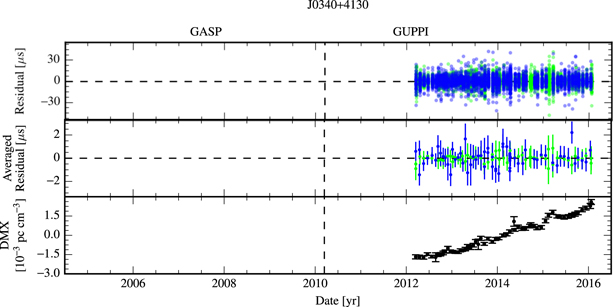
Figure 9. Timing summary for PSR J0340+4130. The colors are defined as follows. Blue: 1.4 GHz. Purple: 2.1 GHz. Green: 820 MHz. Orange: 430 MHz. Red: 327 MHz. In the top panel, individual points are semi-transparent; darker regions arise from the overlap of many points.
Download figure:
Standard image High-resolution image
Figure 10. Timing summary for PSR J0613-0200. The colors are defined as follows. Blue: 1.4 GHz. Purple: 2.1 GHz. Green: 820 MHz. Orange: 430 MHz. Red: 327 MHz. In the top panel, individual points are semi-transparent; darker regions arise from the overlap of many points.
Download figure:
Standard image High-resolution image
Figure 11. Timing summary for PSR J0636+5128. The colors are defined as follows. Blue: 1.4 GHz. Purple: 2.1 GHz. Green: 820 MHz. Orange: 430 MHz. Red: 327 MHz. In the top panel, individual points are semi-transparent; darker regions arise from the overlap of many points.
Download figure:
Standard image High-resolution image
Figure 12. Timing summary for PSR J0645+5158. The colors are defined as follows. Blue: 1.4 GHz. Purple: 2.1 GHz. Green: 820 MHz. Orange: 430 MHz. Red: 327 MHz. In the top panel, individual points are semi-transparent; darker regions arise from the overlap of many points.
Download figure:
Standard image High-resolution image
Figure 13. Timing summary for PSR J0740+6620. The colors are defined as follows. Blue: 1.4 GHz. Purple: 2.1 GHz. Green: 820 MHz. Orange: 430 MHz. Red: 327 MHz. In the top panel, individual points are semi-transparent; darker regions arise from the overlap of many points.
Download figure:
Standard image High-resolution image
Figure 14. Timing summary for PSR J0931-1902. The colors are defined as follows. Blue: 1.4 GHz. Purple: 2.1 GHz. Green: 820 MHz. Orange: 430 MHz. Red: 327 MHz. In the top panel, individual points are semi-transparent; darker regions arise from the overlap of many points.
Download figure:
Standard image High-resolution image
Figure 15. Timing summary for PSR J1012+5307. The colors are defined as follows. Blue: 1.4 GHz. Purple: 2.1 GHz. Green: 820 MHz. Orange: 430 MHz. Red: 327 MHz. In the top panel, individual points are semi-transparent; darker regions arise from the overlap of many points.
Download figure:
Standard image High-resolution image
Figure 16. Timing summary for PSR J1024-0719. The colors are defined as follows. Blue: 1.4 GHz. Purple: 2.1 GHz. Green: 820 MHz. Orange: 430 MHz. Red: 327 MHz. In the top panel, individual points are semi-transparent; darker regions arise from the overlap of many points.
Download figure:
Standard image High-resolution image
Figure 17. Timing summary for PSR J1125+7819. The colors are defined as follows. Blue: 1.4 GHz. Purple: 2.1 GHz. Green: 820 MHz. Orange: 430 MHz. Red: 327 MHz. In the top panel, individual points are semi-transparent; darker regions arise from the overlap of many points.
Download figure:
Standard image High-resolution image
Figure 18. Timing summary for PSR J1453+1902. The colors are defined as follows. Blue: 1.4 GHz. Purple: 2.1 GHz. Green: 820 MHz. Orange: 430 MHz. Red: 327 MHz. In the top panel, individual points are semi-transparent; darker regions arise from the overlap of many points.
Download figure:
Standard image High-resolution image
Figure 19. Timing summary for PSR J1455-3330. The colors are defined as follows. Blue: 1.4 GHz. Purple: 2.1 GHz. Green: 820 MHz. Orange: 430 MHz. Red: 327 MHz. In the top panel, individual points are semi-transparent; darker regions arise from the overlap of many points.
Download figure:
Standard image High-resolution image
Figure 20. Timing summary for PSR J1600-3053. The colors are defined as follows. Blue: 1.4 GHz. Purple: 2.1 GHz. Green: 820 MHz. Orange: 430 MHz. Red: 327 MHz. In the top panel, individual points are semi-transparent; darker regions arise from the overlap of many points.
Download figure:
Standard image High-resolution imageTable 8. Pulsar-binary Component Masses and Inclination Angles
| PSR | Pulsar Mass (M⊙) | Companion Mass (M⊙) | System Inclination |
|---|---|---|---|
| J1600−3053 |

|

|

|
| J1614−2230 |

|

|

|
| J1713+0747a |

|

|

|
| J1741+1351a |

|

|

|
| B1855+09 |

|

|

|
| J1903+0327a |

|

|

|
| J1909−3744 |

|

|

|
| J1918−0642 |

|

|

|
| J2043+1711 |

|

|

|
Note. All estimates were made using the "traditional" (mc,  ) parameterization of the Shapiro delay. All uncertainties reflect 68.3% credible intervals.
Download table as: ASCIITypeset image
Three binary systems—those of PSRs J1600−3053, J1903+0327, and J2234+0611—show a significant time variation in their periastron arguments ( ). Previous studies using other data sets interpreted the observed
  values for PSR J1903+0327 (Freire et al. 2011) and PSR J2234+0611 (Antoniadis et al. 2016) as being due to general relativistic orbital precession, while F16 used the NG9 data set to conclude the same for the
  of PSR J1600−3053. For PSR J1600−3053, the precision in the
  measurement has improved by a factor of ∼1.7 since NG9, consistent with the expected improvement in measurability of post-Keplerian variations over time (Damour & Taylor 1992); based on this scaling relation, the significance of
  will reach 10σ by ∼2020. The constrained estimates of the Shapiro-delay parameters, have similarly improved, allowing us to measure
  for this pulsar.
Five binary systems show significant variations of their orbital periods over time ( ). For three of these systems—PSRs J1012+5307, J1614−2230, and J1909−3744—previous analyses by Desvignes et al. (2016) and F16 showed that the dominant mechanism for the observed variations is relative acceleration between the solar system barycenter and the binary systems (see Section 4.3). We also measured large orbital-period variations in PSRs J0023+0923 and J0636+5128 for the first time; the timing solution for PSR J0023+0932 fits four significant time derivatives of the orbital frequency nb = 2π/Pb, though only the derived
  is shown in Table 7. A sixth pulsar, PSR J0613−0200, shows a marginally significant
  this was not included in our fit files, as it did not pass the F-test used for parameter significance. However, its value is consistent with the estimate made by Desvignes et al. (2016), and is in agreement with the predicted value from various sources of relative acceleration.

Figure 21. Timing summary for PSR J1614-2230. The colors are defined as follows. Blue: 1.4 GHz. Purple: 2.1 GHz. Green: 820 MHz. Orange: 430 MHz. Red: 327 MHz. In the top panel, individual points are semi-transparent; darker regions arise from the overlap of many points.
Download figure:
Standard image High-resolution image
Figure 22. Timing summary for PSR J1640+2224. The colors are defined as follows. Blue: 1.4 GHz. Purple: 2.1 GHz. Green: 820 MHz. Orange: 430 MHz. Red: 327 MHz. In the top panel, individual points are semi-transparent; darker regions arise from the overlap of many points.
Download figure:
Standard image High-resolution image
Figure 23. Timing summary for PSR J1643-1224. The colors are defined as follows. Blue: 1.4 GHz. Purple: 2.1 GHz. Green: 820 MHz. Orange: 430 MHz. Red: 327 MHz. In the top panel, individual points are semi-transparent; darker regions arise from the overlap of many points.
Download figure:
Standard image High-resolution image
Figure 24. Timing summary for PSR J1713+0747. The colors are defined as follows. Blue: 1.4 GHz. Purple: 2.1 GHz. Green: 820 MHz. Orange: 430 MHz. Red: 327 MHz. In the top panel, individual points are semi-transparent; darker regions arise from the overlap of many points.
Download figure:
Standard image High-resolution image
Figure 25. Timing summary for PSR J1738+0333. The colors are defined as follows. Blue: 1.4 GHz. Purple: 2.1 GHz. Green: 820 MHz. Orange: 430 MHz. Red: 327 MHz. In the top panel, individual points are semi-transparent; darker regions arise from the overlap of many points.
Download figure:
Standard image High-resolution image
Figure 26. Timing summary for PSR J1741+1351. The colors are defined as follows. Blue: 1.4 GHz. Purple: 2.1 GHz. Green: 820 MHz. Orange: 430 MHz. Red: 327 MHz. In the top panel, individual points are semi-transparent; darker regions arise from the overlap of many points.
Download figure:
Standard image High-resolution image
Figure 27. Timing summary for PSR J1744-1134. The colors are defined as follows. Blue: 1.4 GHz. Purple: 2.1 GHz. Green: 820 MHz. Orange: 430 MHz. Red: 327 MHz. In the top panel, individual points are semi-transparent; darker regions arise from the overlap of many points.
Download figure:
Standard image High-resolution image
Figure 28. Timing summary for PSR J1747-4036. The colors are defined as follows. Blue: 1.4 GHz. Purple: 2.1 GHz. Green: 820 MHz. Orange: 430 MHz. Red: 327 MHz. In the top panel, individual points are semi-transparent; darker regions arise from the overlap of many points.
Download figure:
Standard image High-resolution image
Figure 29. Timing summary for PSR J1832-0836. The colors are defined as follows. Blue: 1.4 GHz. Purple: 2.1 GHz. Green: 820 MHz. Orange: 430 MHz. Red: 327 MHz. In the top panel, individual points are semi-transparent; darker regions arise from the overlap of many points.
Download figure:
Standard image High-resolution image
Figure 30. Timing summary for PSR J1853+1303. The colors are defined as follows. Blue: 1.4 GHz. Purple: 2.1 GHz. Green: 820 MHz. Orange: 430 MHz. Red: 327 MHz. In the top panel, individual points are semi-transparent; darker regions arise from the overlap of many points.
Download figure:
Standard image High-resolution image
Figure 31. Timing summary for PSR B1855+09. The colors are defined as follows. Blue: 1.4 GHz. Purple: 2.1 GHz. Green: 820 MHz. Orange: 430 MHz. Red: 327 MHz. In the top panel, individual points are semi-transparent; darker regions arise from the overlap of many points.
Download figure:
Standard image High-resolution image
Figure 32. Timing summary for PSR J1903+0327. The colors are defined as follows. Blue: 1.4 GHz. Purple: 2.1 GHz. Green: 820 MHz. Orange: 430 MHz. Red: 327 MHz. In the top panel, individual points are semi-transparent; darker regions arise from the overlap of many points.
Download figure:
Standard image High-resolution image
Figure 33. Timing summary for PSR J1909-3744. The colors are defined as follows. Blue: 1.4 GHz. Purple: 2.1 GHz. Green: 820 MHz. Orange: 430 MHz. Red: 327 MHz. In the top panel, individual points are semi-transparent; darker regions arise from the overlap of many points.
Download figure:
Standard image High-resolution image
Figure 34. Timing summary for PSR J1910+1256. The colors are defined as follows. Blue: 1.4 GHz. Purple: 2.1 GHz. Green: 820 MHz. Orange: 430 MHz. Red: 327 MHz. In the top panel, individual points are semi-transparent; darker regions arise from the overlap of many points.
Download figure:
Standard image High-resolution imageFor PSRs J0023+0923 and J0636+5128, short periods (∼3 hr) and very-low minimum companion masses (mc,min ∼0.05 M⊙) suggest these are black widow systems, in which torques produced from tidal interactions with an oblate companion can cause orbital variability (e.g., Applegate & Shaham 1994). Recent simulations of long-term variability in black widow systems have shown that such behavior will not significantly impact the detection of nHz-frequency GWs (Bochenek et al. 2015). However, long-term timing of the PSR J2051−0827 black widow system illustrated apparent variations in x, the projected semimajor axis, that may also need to be accounted for in such systems (Shaifullah et al. 2016).

Figure 35. Timing summary for PSR J1911+1347. The colors are defined as follows. Blue: 1.4 GHz. Purple: 2.1 GHz. Green: 820 MHz. Orange: 430 MHz. Red: 327 MHz. In the top panel, individual points are semi-transparent; darker regions arise from the overlap of many points.
Download figure:
Standard image High-resolution image
Figure 36. Timing summary for PSR J1918-0642. The colors are defined as follows. Blue: 1.4 GHz. Purple: 2.1 GHz. Green: 820 MHz. Orange: 430 MHz. Red: 327 MHz. In the top panel, individual points are semi-transparent; darker regions arise from the overlap of many points.
Download figure:
Standard image High-resolution image
Figure 37. Timing summary for PSR J1923+2515. The colors are defined as follows. Blue: 1.4 GHz. Purple: 2.1 GHz. Green: 820 MHz. Orange: 430 MHz. Red: 327 MHz. In the top panel, individual points are semi-transparent; darker regions arise from the overlap of many points.
Download figure:
Standard image High-resolution image
Figure 38. Timing summary for PSR B1937+21. The colors are defined as follows. Blue: 1.4 GHz. Purple: 2.1 GHz. Green: 820 MHz. Orange: 430 MHz. Red: 327 MHz. In the top panel, individual points are semi-transparent; darker regions arise from the overlap of many points.
Download figure:
Standard image High-resolution image
Figure 39. Timing summary for PSR J1944+0907. The colors are defined as follows. Blue: 1.4 GHz. Purple: 2.1 GHz. Green: 820 MHz. Orange: 430 MHz. Red: 327 MHz. In the top panel, individual points are semi-transparent; darker regions arise from the overlap of many points.
Download figure:
Standard image High-resolution image
Figure 40. Timing summary for PSR B1953+29. The colors are defined as follows. Blue: 1.4 GHz. Purple: 2.1 GHz. Green: 820 MHz. Orange: 430 MHz. Red: 327 MHz. In the top panel, individual points are semi-transparent; darker regions arise from the overlap of many points.
Download figure:
Standard image High-resolution image
Figure 41. Timing summary for PSR J2010-1323. The colors are defined as follows. Blue: 1.4 GHz. Purple: 2.1 GHz. Green: 820 MHz. Orange: 430 MHz. Red: 327 MHz. In the top panel, individual points are semi-transparent; darker regions arise from the overlap of many points.
Download figure:
Standard image High-resolution image
Figure 42. Timing summary for PSR J2017+0603. The colors are defined as follows. Blue: 1.4 GHz. Purple: 2.1 GHz. Green: 820 MHz. Orange: 430 MHz. Red: 327 MHz. In the top panel, individual points are semi-transparent; darker regions arise from the overlap of many points.
Download figure:
Standard image High-resolution image
Figure 43. Timing summary for PSR J2033+1734. The colors are defined as follows. Blue: 1.4 GHz. Purple: 2.1 GHz. Green: 820 MHz. Orange: 430 MHz. Red: 327 MHz. In the top panel, individual points are semi-transparent; darker regions arise from the overlap of many points.
Download figure:
Standard image High-resolution image
Figure 44. Timing summary for PSR J2043+1711. The colors are defined as follows. Blue: 1.4 GHz. Purple: 2.1 GHz. Green: 820 MHz. Orange: 430 MHz. Red: 327 MHz. In the top panel, individual points are semi-transparent; darker regions arise from the overlap of many points.
Download figure:
Standard image High-resolution image
Figure 45. Timing summary for PSR J2145-0750. The colors are defined as follows. Blue: 1.4 GHz. Purple: 2.1 GHz. Green: 820 MHz. Orange: 430 MHz. Red: 327 MHz. In the top panel, individual points are semi-transparent; darker regions arise from the overlap of many points.
Download figure:
Standard image High-resolution image
Figure 46. Timing summary for PSR J2214+3000. The colors are defined as follows. Blue: 1.4 GHz. Purple: 2.1 GHz. Green: 820 MHz. Orange: 430 MHz. Red: 327 MHz. In the top panel, individual points are semi-transparent; darker regions arise from the overlap of many points.
Download figure:
Standard image High-resolution image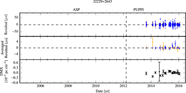
Figure 47. Timing summary for PSR J2229+2643. The colors are defined as follows. Blue: 1.4 GHz. Purple: 2.1 GHz. Green: 820 MHz. Orange: 430 MHz. Red: 327 MHz. In the top panel, individual points are semi-transparent; darker regions arise from the overlap of many points.
Download figure:
Standard image High-resolution image
Figure 48. Timing summary for PSR J2234+0611. The colors are defined as follows. Blue: 1.4 GHz. Purple: 2.1 GHz. Green: 820 MHz. Orange: 430 MHz. Red: 327 MHz. In the top panel, individual points are semi-transparent; darker regions arise from the overlap of many points.
Download figure:
Standard image High-resolution image
Figure 49. Timing summary for PSR J2234+0944. The colors are defined as follows. Blue: 1.4 GHz. Purple: 2.1 GHz. Green: 820 MHz. Orange: 430 MHz. Red: 327 MHz. In the top panel, individual points are semi-transparent; darker regions arise from the overlap of many points.
Download figure:
Standard image High-resolution image
Figure 50. Timing summary for PSR J2302+4442. The colors are defined as follows. Blue: 1.4 GHz. Purple: 2.1 GHz. Green: 820 MHz. Orange: 430 MHz. Red: 327 MHz. In the top panel, individual points are semi-transparent; darker regions arise from the overlap of many points.
Download figure:
Standard image High-resolution image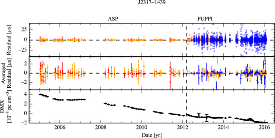
Figure 51. Timing summary for PSR J2317+1439. The colors are defined as follows. Blue: 1.4 GHz. Purple: 2.1 GHz. Green: 820 MHz. Orange: 430 MHz. Red: 327 MHz. In the top panel, individual points are semi-transparent; darker regions arise from the overlap of many points.
Download figure:
Standard image High-resolution image
Many of our binary pulsars exhibit significant changes in their projected semimajor axes over time ( ). The dominant mechanism for these observed variations is the change in apparent inclination of the orbital plane due to proper motion of the system (Kopeikin 1996). F16 used the observed Shapiro delay and
  in the PSR J1741+1351 system to directly estimate a value for the longitude of ascending node (Ω), along with the masses and system inclination. We find that Ω =330° ± 30°, consistent with the measurement of 317° ± 35° in F16.
6. Summary and Conclusions
We have presented the timing data and analysis for 45 millisecond pulsars observed for time spans of up to 11 years from the NANOGrav timing program. We outlined the analysis procedure used to calculate TOAs and fit these TOAs to models including spin, astrometric, and binary (if necessary) parameters, along with a parameterized noise model for each pulsar. The timing and noise analysis methods used for the 11-year data set are nearly identical to those described in our previous (9-year) data set paper, Arzoumanian et al. (2015b). However, we made several improvements to the initial stages of preparing the TOAs for fitting. We incorporated a more sophisticated, automated analysis to identify outlier TOAs. We also excluded data with insufficient radio-frequency coverage to fit an accurate DM. In addition, we adjusted the criterion for DM-epoch determination for data for which a solar wind model predicted large delays. These improvements provided greater immunity to corruption of timing- and noise-model parameters due to instrumental effects or unmodeled dispersive delays.
In general, timing solutions are comparable with NG9, with reduced uncertainties on timing-derived parameters. We measured several timing parameters for the first time in the 11-year data set. We measured parallaxes of 20 pulsars, 3 for the first time (PSRs J0740+6620, J2334+0611, and J2234+0944). We measured Shapiro delay for PSRs J0740+6620 and J1853+1303 for the first time ever, and improved the Shapiro-delay measurements, and hence mass estimates, for an additional 14 pulsars. Large orbital-period variations have been measured for two pulsars (PSRs J0023+0923 and J0636+5128) for the first time. We attribute these variations to torques produced by tidal interactions with their low-mass companions.
Our noise analysis indicates that 11 pulsars show evidence for significant red noise, i.e., noise with power peaking at lower frequencies. Because we have excluded data with insufficient frequency coverage for reliable dispersion-delay measurements, and those with large predicted unmodeled solar-wind delays, in most cases we cannot attribute this red noise to interstellar-medium effects. All of the pulsars with well constrained red-noise spectral indices show low values, ranging from −1 to −3, indicating flatter spectra than observed for normal pulsars, for which red noise has been attributed to intrinsic spin noise. If the red noise is intrinsic, this may suggest a different origin in millisecond pulsars. Most importantly, the spectral indices are less steep than the −11/3 predicted for the stochastic gravitational-wave background, indicating that we should continue to gain in sensitivity as the time span of our data set grows.
NANOGrav is committed to publicly releasing its timing data on a regular basis. This data set is the third NANOGrav release. As with previously released data sets, the data described in this paper are being used to constrain the presence of gravitational waves due to a stochastic background of supermassive black hole binaries (Arzoumanian et al. 2018). They will also be used to search for single (or continuous-wave) sources and for burst sources. Future papers will detail these analyses and their astrophysical implications. These data represent a significant increase in sensitivity over the nine-year set, which contained 37 pulsars. As we continue to add pulsars to the array, and as the total time span lengthens, our sensitivity to gravitational waves will grow, with a detection expected within the next 5–6 years (Taylor et al. 2016).
The author list reflects the broad variety of contributions of authors to the NANOGrav project. Some specific contributions to this paper, particularly incremental work between NG9 and the present work, are as follows. Z.A., K.C., P.B.D., T.D., E.F., R.D.F., E.F., P.A.G., C.J., G.J., D.H., M.T.L., L.L., D.R.L., R.S.L., M.A.M., C.N., D.J.N., T.T.P., S.M.R., R.S., I.H.S., K.S., J.K.S., and W.Z. each made at least 20 hr of observations for this project. M.E.D., E.F., M.J., M.T.L., D.R.L., M.A.M., C.N., D.J.N., T.T.P., P.S.R., S.M.R., and I.H.S. generated and checked timing solutions for individual pulsars. P.B.D., M.E.D., J.A.E., R.D.F., M.T.L., C.N., D.J.N., and I.H.S. developed and refined procedures and computational tools for the timing pipeline. R.v.H., M.V., and J.A.E. implemented the TOA outlier-detection procedure. P.B.D. wrote observing proposals, coordinated Green Bank observations, performed calibration and TOA generation, coordinated the data flow, developed the data files for public release, and contributed substantially to the text. J.A.E. developed and refined the algorithms and software implemented used for the noise model. He wrote substantial amounts of the text, and contributed several tables and figures. D.J.N. coordinated the development of the data set and the writing of this paper, co-authored observing proposals, chaired the NANOGrav Timing Working Group, undertook some of the astrometric analysis, and wrote portions of the text. I.H.S. coordinated the Arecibo observations. E.F. wrote observing proposals, assisted in coordination of Arecibo observations, and undertook the analysis and write-up of binary pulsars in Section 5. A.M. undertook the analysis and write-up of parallax and distance measurements in Section 4.
The NANOGrav project receives support from National Science Foundation (NSF) Physics Frontiers Center award number 1430284. Pulsar research at UBC is supported by an NSERC Discovery Grant and by the Canadian Institute for Advanced Research. The Arecibo Observatory is operated by SRI International under a cooperative agreement with the NSF (AST-1100968), and in alliance with Ana G. Méndez-Universidad Metropolitana, and the Universities Space Research Association. The Green Bank Observatory is a facility of the National Science Foundation operated under cooperative agreement by Associated Universities, Inc. Part of this research was carried out at the Jet Propulsion Laboratory, California Institute of Technology, under a contract with the National Aeronautics and Space Administration. The Flatiron Institute is supported by the Simons Foundation. The Dunlap Institute is funded by an endowment established by the David Dunlap family and the University of Toronto. J.A.E. was partially supported by NASA Einstein Fellowship grant PF4-150120. R.v.H. was supported by NASA Einstein Fellowship grant PF3-140116. W.W.Z. is supported by the CAS Pioneer Hundred Talents Program and the Strategic Priority Research Program of the Chinese Academy of Sciences, grant No. XDB23000000.
Software: PSRCHIVE (Hotan et al. 2004), nanopipe (Demorest 2018), Tempo (Nice et al. 2015), Tempo2 (Edwards et al. 2006; Hobbs et al. 2006), PAL2 (Ellis & van Haasteren 2017a), PTMCMCSampler (Ellis & van Haasteren 2017b), MultiNest (Feroz et al. 2009).
Appendix: Daily Averaged Residuals
This appendix includes plots of residual time series and DM variations for each pulsar in our data set.
As described in Section 2, each observation in our data set produced a large number of arrival times representing data collected simultaneously over a range of radio-frequency bands. The top panel of each figure in this appendix shows the residual arrival time (observed minus computed) for every arrival time measurement in the data set for a given pulsar. Points in the plots are colored based on receiver frequency, and the predominant data-collection instrument over any given time period is indicated at the top of each plot, with vertical dashed lines indicating times at which data-collection instruments changed.
The models used for residual plots include the effect of red noise, but any red noise corresponding to a linear or quadratic trend has been removed, as it is completely covariant with pulsar rotation frequency and frequency derivative in the timing model, and hence would be absorbed by fits for these quantities.
Daily-average residuals for each receiver are shown in the second panel for each pulsar. These were computed using the procedure described in Appendix D of NG9.
For pulsars whose timing models include red noise (Table 2), the third panel of the figure shows whitened residuals, which were calculated by subtracting the red-noise model from the daily-average residuals.
The bottom panel of each figure shows the variation in DM for each pulsar. These are presented as DMXi ≡ DMi–DMaverage, where DMi is the DM at epoch i and DMaverage is the average DM over the entire data set for the pulsar. Lengths of epochs are described in Section 2, and are typically 6 days or less, except in the earliest data. Subtracting the average value is advantageous because it allows us to remove the uncertainty in DMaverage (which arises due to covariance with the FD parameters described in Section 2) from the uncertainties in DMXi shown in the figures.
Footnotes
- 37
North American Nanohertz Observatory for Gravitational Waves; http://nanograv.org.
- 38
- 39
- 40
- 41
- 42
- 43
The final noise analysis assumes Gaussian noise after outliers have been removed.
- 44
- 45
Random walks in pulsar phase, period, and period derivative lead to underlying power spectral indices of −2, −4, and −6, respectively (Shannon & Cordes 2010).
- 46